Evolving Deep DenseBlock Architecture Ensembles for Image Classification

Abstract

Automatic deep architecture generation is a challenging task, owing to the large number of controlling parameters inherent in the construction of deep networks. The combination of these parameters leads to the creation of large, complex search spaces that are feasibly impossible to properly navigate without a huge amount of resources for parallelisation. To deal with such challenges, in this research we propose a Swarm Optimised DenseBlock Architecture Ensemble (SODBAE) method, a joint optimisation and training process that explores a constrained search space over a skeleton DenseBlock Convolutional Neural Network (CNN) architecture. Specifically, we employ novel weight inheritance learning mechanisms, a DenseBlock skeleton architecture, as well as adaptive Particle Swarm Optimisation (PSO) with cosine search coefficients to devise networks whilst maintaining practical computational costs. Moreover, the architecture design takes advantage of recent advancements of the concepts of residual connections and dense connectivity, in order to yield CNN models with a much wider variety of structural variations. The proposed weight inheritance learning schemes perform joint optimisation and training of the architectures to reduce the computational costs. Being evaluated using the CIFAR-10 dataset, the proposed model shows great superiority in classification performance over other state-of-the-art methods while illustrating a greater versatility in architecture generation.

1. Introduction

Automatic deep architecture design is a growing practice within the domain of deep learning. The rapid pace of deep learning research has brought continued advancements in tools and methods for network generation. Many architecture generation/optimisation studies [1,2,3,4,5] focus on attempting to design deep networks from primitive building blocks, allowing for their methods to generate a huge variety of potential architectures. Such strategies are interesting but create search spaces that are enormous and feasibly impossible to properly navigate without a huge amount of resources for parallelisation. In this research, we propose novel weight inheritance training schemes, a DenseBlock skeleton architecture, in conjunction with adaptive Particle Swarm Optimisation (PSO) with cosine search trajectories, in order to improve efficiency while generating diverse architectures.

Specifically, in this research, we propose a Swarm Optimised DenseBlock Architecture Ensemble (SODBAE) method, a joint optimisation and training process that explores a constrained search space over a skeleton DenseBlock Convolutional Neural Network (CNN) architecture. We conduct the architecture search while using a PSO variant with adaptive cosine search coefficients to balance between exploration and exploitation. Importantly, in order to significantly improve computational efficiency, two weight inheritance learning schemes, i.e., Block Lookup Size Key-Name and Size (BLSK-NS), and Block Lookup Size Key-Size (BLSK-S), are proposed for joint optimisation and training of the CNN architectures. Precisely, the individual particles are jointly optimised and trained while using the above proposed continual training strategies that operate on the individual layers of the network. These weight inheritance schemes are subsequently applied to any CNN architecture devised by the swarm particles and utilise combinations of the name of the layer and the size of its parameter matrix to construct search keys for the centralised lookup tables. Following the aforementioned optimisation and training process, ensemble classification models are constructed from local best positions, as well as the distinctive particles from the final iteration in order to take advantage of the diversity of the jointly trained models.

The research contributions are as follows.

• A deep ensemble architecture optimisation method is proposed for devising ensembles of deep neural networks while using dense connectivity principles.
• A DenseBlock-based skeleton architecture is proposed for effective optimisation.
• Two weight inheritance strategies, i.e., the BLSK-NS and BLSK-S methods, are proposed for the joint optimisation and training of complex CNN architectures.
• A comprehensive evaluation of the devised ensemble and base CNN models using various weight inheritance configurations on the CIFAR-10 dataset is provided.

The proposed SODBAE model provides an automatic approach for densely connected CNN model generation. Additionally, the BLSK-NS and BLSK-S weight inheritance methods provide continual training to any selection of CNN networks by functioning over the individual layers of a network. The proposed approach is able to devise sophisticated deep networks with versatile architectures while maintaining a reasonable trade-off between performance and computational efficiency.

2. Related Work

Automatic CNN architecture generation/optimisation and hyper-parameter fine-tuning have drawn great attention in computer vision [6]. In parallel, evolutionary algorithms, such as PSO, show significant search capabilities in solving a variety of optimization problems. Proposed by Kennedy and Eberhart [7], the PSO algorithm employs the personal and global best experiences to guide the swarm to search for global optimality. Equations (1) and (2) define the velocity and position updating operations of the original PSO algorithm.

$$v_i^{t+1}=w{v}_i^t+c_1{r}_1(pbes{t}_i^t-x_i^t)+c_2{r}_2(gbes{t}^t-x_i^t)$$

(1)

$$x_i^{t+1}=x_i^t+v_i^{t+1}$$

(2)

where $v_i^{t+1}$ and $x_i^{t+1}$ represent the velocity and position of particle i in the ($t+1$)-th iteration, with w representing the inertia weight. The personal best solution of the particle i is denoted as $pbes{t}_i$, while the global best solution is represented as $gbest$. The acceleration coefficients $c_1$ and $c_2$ determine the focus of the search process between the cognitive and social components, with $r_1$ and $r_2$ representing the random search parameters. The acceleration coefficients $c_1$ and $c_2$ are assigned as constant values in the original PSO algorithm. As indicated in Equations (1) and (2), the particle velocity and position updating operations are guided by the personal and global best solutions to move the swarm towards global optimality.

The PSO algorithm has been widely adopted for optimal architecture generation and hyper-parameter fine-tuning applications. As an example, Yamasaki et al. [8] conducted optimal hyper-parameter selection with respect to AlexNet while using the PSO algorithm. Their work optimised several key configuration settings such as the kernel sizes, padding, the number of filters, and types of pooling, for optimal network identification. The ranking correlation and volatility strategies were proposed in order to optimise computational efficiency at the training stage. The PSO-optimised AlexNet model obtained accuracy rates of $80.15\%$ and $53.28\%$ for the CIFAR-10 and CIFAR-100 datasets, respectively. Domhan et al. [9] proposed strategies to accelerate optimal hyper-parameter identification for deep networks. A probabilistic learning curve mechanism was proposed in order eliminate learning options that were very unlikely to result in optimal performances in early training stages. A comprehensive evaluation was conducted for the optimisation of a number of learning configurations for both small and large networks, which included network hyper-parameters (such as initial learning rate, learning rate decay, momentum, weight decay, dropout rate, and the number of pooling layers), as well as convolutional layer hyper-parameters (such as the number of units, weight filler type (Gaussian and Xavier), and weight learning rate multiplier). Evaluated with the CIFAR-10 dataset, the optimised small and large CNN models obtained error rates of $17.2\%$ and $8.81\%$, respectively, for image classification tasks. Lievski et al. [10] proposed a mixed integer deterministic-surrogate optimisation algorithm, namely Hyper-parameter Optimisation using radial basis function (RBF) and Dynamic coordinate search (HORD), for hyper-parameter identification in deep networks. Specifically, the RBF interpolation model was employed as the error surrogates for optimal hyper-parameter search. Besides that, the new offspring solutions were yielded in the close neighbourhood of the current global best solution in each iteration to significantly reduce the number of evaluations. The model showed superior performances for both low and high dimensional hyper-parameter optimisation problems when evaluated with four deep neural networks with six, eight, 15, and 19 hyper-parameters, respectively. Their work obtained an error rate of $20.54\%$ for the CIFAR-10 dataset by optimising a CNN model with 19 hyper-parameters.

Albelwi and Mahmood [11] proposed the Nelder–Mead Method (NMM) in conjunction with a newly proposed objective function based on the error rate and the quality of the feature visualization using deconvolutional networks for deep architecture optimisation. Their objective function was able to reduce the error rate and improve the visualization results of the feature maps simultaneously. Because reconstructing images using feature activations was an effective way to indicate model efficiency, their work subsequently generated a correlation coefficient score between a pair of the original input and the reconstructed images for quality measurement. The hyper-parameters, such as the depths of convolutional and fully-connected layers, the number of filters, the kernel sizes, the number of pooling layers, pooling region sizes, and the number of neurons in fully-connected layers were optimised. Evaluated while using the CIFAR-10 dataset, their work achieved an error rate of $10.05\%$ for image classification. Tan et al. [3] proposed a PSO variant for deep CNN architecture generation for skin cancer classification. The search of the optimal network topology was conducted based on an initial skeleton network with distinctive block architectures. The optimisation objective was to identify optimal training hyper-parameters (e.g., learning rate and weight decay), and the numbers of distinctive convolutional blocks with differentiated feature map sizes. Their PSO variant hybridized with crossover, mutation, and spiral search operations as well as attraction actions guided by the mean and randomly selected positions of the neighbouring elite solutions. Besides the deep architecture generation, the model was also used to enhance the lesion-skin segmentation performance by further enhancing the cluster centroids identified by the K-Means clustering. Evaluated with several well-known skin lesion datasets, such as ISIC 2017, the model outperformed a number of advanced PSO algorithms [12,13,14] for architecture generation and foreground-background segmentation for melanoma classification. Sun et al. [15] proposed automatic PSO-based architecture generation based on the proposal of flexible convolutional autoencoders, while Liang [16] performed the optimisation of fully connected (FC) layers in CNN models and Liu et al. [17] employed multi-objective optimisation for the design of optimal layer structures in deep networks.

Lu et al. [18] devised deep networks while using the Bayesian optimisation algorithm for an electrochemical drilling process. First, a network architecture consisting of a convolutional layer followed by three dense layers was determined based on manual trial-and-error. The Bayesian algorithm optimised the following CNN network hyper-parameters, i.e., the training-validation split, the dropout ratio, the numbers of neurons in the three dense layers, and the training iterations. Random dropout layers were also implanted to the generated networks in order to avoid overfitting. The Bayesian-optimised CNN model outperformed a physics embedded neural network and a Support Vector Regression (SVR) model for the prediction of the diameters of the drilled holes in electrochemical drilling tasks. Zhang et al. [19] proposed ensemble transfer learning models for optic disc (OD) segmentation with PSO-based hyper-parameter identification. Mask R-CNN was employed as the base evaluator. A new PSO algorithm was proposed in order ro optimise the hyper-parameters of each base segmenter. It comprised a number of mechanisms, such as accelerated and refined search actions with versatile super-ellipse trajectories, a super-formula oriented leader enhancement, as well as mean and random leader-guided search operations, to mitigate early stagnation. In order to further test model efficiency, the PSO algorithm was also evaluated using benchmark test functions, as well as hyper-parameter fine-tuning of the VGG16 model for a diagnostic problem, i.e., the detection of Diabetic Macular Edema (DME). Evaluated using Messidor and Drions datasets, their PSO-based ensemble transfer learning models showed superior performance over those yielded while using classical and advanced search methods, as well as state-of-the-art related studies based on handcrafted features, for OD segmentation and DME classification. Junior and Yen [5] devised deep architectures based on a modified PSO operation where each particle with a variable length was used to denote a potential deep CNN topology. New operators for the calculation of position difference and velocity updating were proposed to facilitate the optimal deep architecture search. Their optimised CNN networks achieved superior performance for MNIST and a number of its variant datasets with respect to image classification tasks.

3. Materials and Methods

3.1. Search Space Design

Deep architecture generation is a challenging task, since related studies [1,2,4,20] tend to create search spaces that are immense and feasibly impossible to properly navigate without a huge amount of resources for parallelisation. In this research, we approach the problem differently by proposing novel weight inheritance schemes, a DenseBlock skeleton architecture, as well as an adaptive cosine oriented PSO search mechanism to balance between devising versatile architectures and maintaining optimal training costs. In addition, we devise the skeleton architecture by considering more recent developments in the world of CNN design. Specifically, we employ the concept of residual or skip connections [21], as well as the concept of dense connectivity [22], in order to create architectures from a set of parameters with a much wider variety of structural variations. Using our DenseBlock skeleton architecture, we obtain a search process to include a total of $K\times D^{i-1}$ potential architectures, where K represents the denormalised range of the growth rate (k), while D represents the denormalised range of the depth (number of internal layers) of each dense block, and i represents the number of dense blocks. Such a potentially large search space provides a vastly more difficult task, albeit with the benefit of greater oautonomyn the part of the optimisation process. To significantly reduce computational costs and effectively explore the search space, two weight inheritance strategies, i.e., the BLSK-NS and BLSK-S methods, are proposed for the joint optimisation and training of the CNN architectures. These weight inheritance strategies purely rely on the parameters of the individual layers in the CNN architecture, meaning they can be used with any CNN construction method, rather than being tied to the optimisation process itself. Two ensemble models are subsequently built based on the optimised deep networks with dense connectivity to further enhance performance. We introduce each key proposed strategy comprehensively below.

Model Construction

Similar to the VGG networks, a typical DenseNet CNN model for image classification is constructed as a hierarchical graph of convolutional, batch normalisation, ReLU activation, and average pooling layers, followed by a final fully connected classification layer and a Softmax output layer. However, whilst the VGG models attach the output of a layer only with the next contiguous layer, DenseNets build up a ‘global state’ by connecting the output of a layer with all of the subsequent layers. This global state takes the form of a stack of feature maps, where the output of a layer is simply concatenated onto the stack following its processing of the previous global state. Constructing the network in this way allows the features from earlier in the network to persist for longer in the network hierarchy, rather than being repeatedly reprocessed by the intermediate layers and losing entropy.

Moreover, in the proposed DenseBlock skeleton architecture, as many existing studies [3,5,15], we employ the concept of blocks separated by spatial downsampling layers, in order to reduce the spatial size of the feature maps and increase the receptive field size of the subsequent layers. However, we achieve this by using the DenseNet concept of the ‘growth rate’ (k), which defines the number of feature maps that each new layer can concatenate onto the global state matrix. The growth rate is also used to determine the maximum size of the global state, as an excessive growth rate can result in drastically reduced performance. 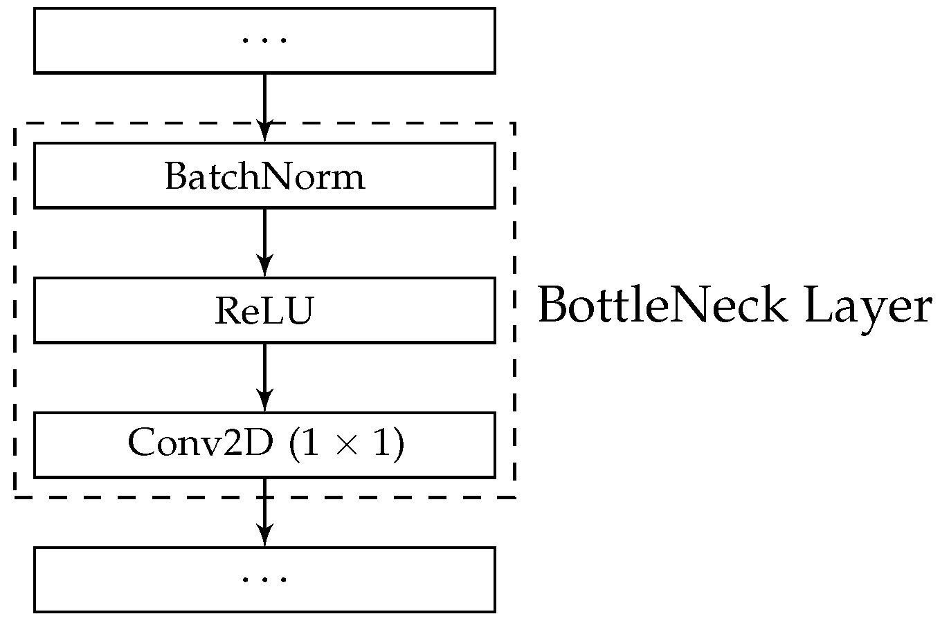In our experiments, we set the maximum size of the global state as $4k$, based on the recommendation of [22]. This maximum size is maintained through the use of BottleNeck Layers consisting of a batch normalisation layer, followed by a ReLU activation and a $1\times 1$ convolution mapping the number of input features to the maximum global state size. A visualisation of a BottleNeck Layer can be seen in Figure 1.

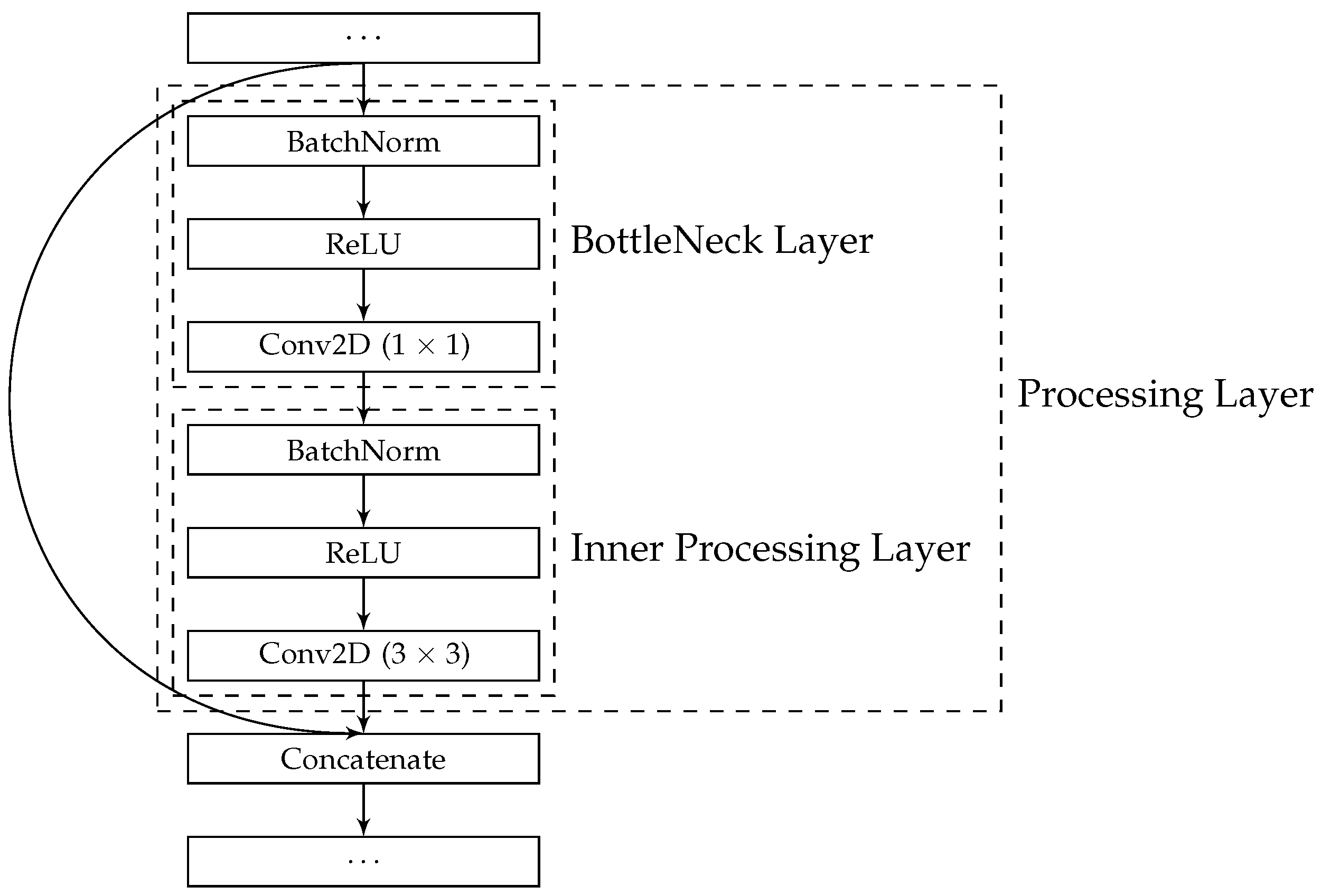
As compared with related studies, including a BottleNeck layer before every convolution creates a fundamental change in structure, resulting in a definition of Processing Layers that are stacked within the blocks of our resulting architectures. Figure 2 depicts the Processing Layer definition, which consists of a sequence of actual component layers, i.e., batch normalisation, ReLU Activation, $1\times 1$ convolution, batch normalisation, ReLU Activation, and finally a $3\times 3$ convolution to form the bulk of the processing.

One effect of the number of feature maps produced and processed by the Processing Layers is that the parameter matrices do not grow to enormous sizes. This allows for us to construct much deeper networks by stacking many more Processing Layers in each block, without running out of GPU memory in the process. Due to the dense connections that are inherent in the SODBAE skeleton architecture, we also do not suffer from the vanishing entropy problem commonly seen when drastically increasing the depth of a CNN. Moreover, the optimization process enables each processing layer to always add the identified optimal (e.g., k) number of feature maps to the global state. We do not enforce any constraints when adding the number of feature maps that are recommended by the optimization process. The maximum number of feature maps in the global state is maintained by the bottleneck layers, as illustrated in Figure 1. Each bottleneck layer uses a 1 × 1 convolution to map the number of input features to the maximum size of the global state, after adding each set of new feature maps from each processing layer.

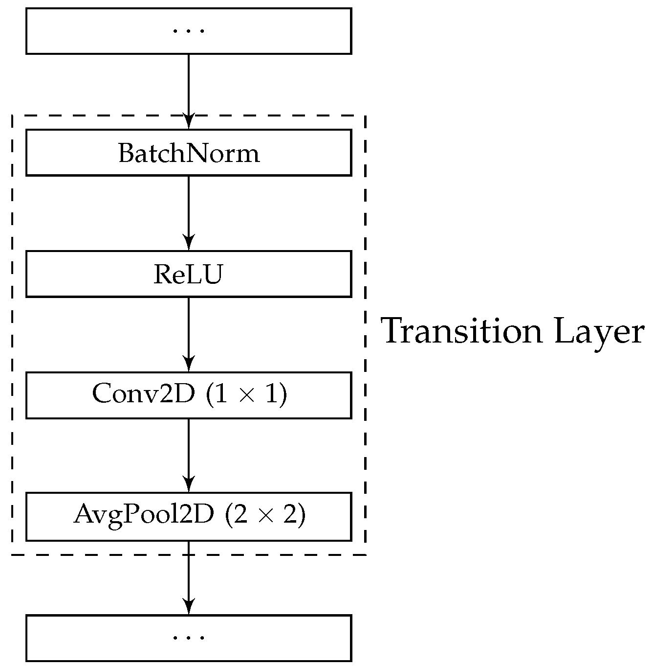
As previously mentioned, in order to periodically reduce the spatial size of the internal feature maps, and increase the receptive field size of later Processing Layers, we implement spatial downsampling between the blocks in the SODBAE skeleton architecture. The spatial downsampling is performed by Transition Layers, rather than simply a single average pooling layer as in many existing studies. Transition Layers, as seen in [22], consist of a batch normalisation layer, followed by a ReLU activation, a $1\times 1$ convolution, and finally an average pooling layer in order to perform the actual spatial downsampling. A visualisation of a Transition Layer can be seen in Figure 3.

In the proposed model, we construct a SODBAE skeleton architecture by defining a number of design choices as parameters to an objective function, where the objective function can then use the parameters with the skeleton architecture in order to construct a full CNN model. The objective function used by the SODBAE method can be seen in Algorithm 1. For the model initialisation process, the skeleton architecture design choices we choose to optimise include:

• The growth rate (k)
• The depth (No. of layers) of the first DenseBlock ($d_0$)
• The depth (No. of layers) of the second DenseBlock ($d_1$)
• The depth (No. of layers) of the third DenseBlock ($d_2$)
• The depth (No. of layers) of the fourth DenseBlock ($d_3$)

Algorithm 1 The objective function to be optimised.

1: functionObjectiveFunction($position$): 2:       model ← InitModel(position) 3:       if weight_sharing then 4:             model.weights ← InheritWeights(model) 5:       end if 6:       Train(model) 7:       error_rate ← Validate(model) 8:       if weight_sharing then 9:             StoreWeights(model, error_rate) 10:     end if 11:     return (error_rate/100) 12: end function

We use ranges of $k=[1,\dots ,48]$ giving $K=48$ for the growth rate and $d=[0,\dots ,48]$ giving $D=49$ for the depth of each dense block, with a total number of blocks of $i=4$. This means that each dense block will consist of between 0 and 48 Processing Layers, with each Processing Layer adding between 1 and 48 feature maps to the global state, which will contain a range of 4 to 192 feature maps at a time. Being motivated by [22], we simply use a single fully connected layer, followed by a Softmax layer to perform the final predictions. As with the earlier reduction in feature maps, this again saves GPU memory, allowing for us to construct deeper models with more convolutional processing.

Table 1. The parameters of the DenseBlock convolutional architecture to be optimised.

Growth Rate (k)	$[1,\dots ,48]$
Denseblock 0 Depth	$[0,\dots ,48]$
Denseblock 1 Depth	$[0,\dots ,48]$
Denseblock 2 Depth	$[0,\dots ,48]$
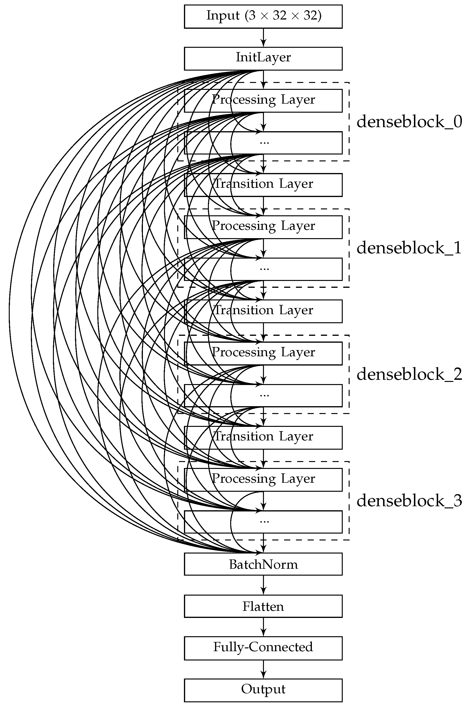
Denseblock 3 Depth	$[0,\dots ,48]$

shows the parameters of the DenseBlock skeleton architecture to be optimised, leading to the total distinct architecture variants of $276,710,448$. The skeleton architecture of the resulting CNN is visualised in Figure 4, where the Processing Layer refers to an encompassing SODBAE Processing Layer, as depicted in Figure 2 and Transition Layer refers to the one, as depicted in Figure 3. The ellipses in the visualisations represent the repeating layers in the respective blocks, where the dense connections will continue between the repeated layers and all subsequent layers, potentially creating very deep, very densely connected architectures. It is important to note that, whilst the dense connections are shown throughout the network, in actual processing this is represented as a global state that passes linearly through the network, allowing for the spatial size of the feature maps inside to be downsampled by the Transition Layers.

3.2. Particle Swarm Optimisation

With the proposed DenseBlock skeleton architecture defined, we subsequently optimise both the growth rate and size of each block by encoding the parameters as dimensions in a swarm optimisation process. The PSO model is selected for deep network generation in this research, owing to its superior search capabilities in solving diverse optimisation problems [23,24,25,26]. Specifically, the proposed SODBAE model utilises a PSO variant where the acceleration coefficients are implemented by adaptive cosine functions, as defined in (3), to optimise the DenseBlock architecture that is described above. According to Mirjalili et al. [27], the acceleration coefficients defined in (3) while using the cosine functions provide comparatively smoother transitions of the search focus between the personal and global best solutions, in comparison with linearly increasing and decreasing search parameters for the social and cognitive components. Such adaptive search parameters enable the model to focus on global exploration at the beginning of the search process to thoroughly explore the search space, and gradually switch to local exploitation towards the final iterations to increase intensification around the global best solution. Therefore, the proposed model is equipped with enhanced capabilities in overcoming local optima traps and finding global optimality.

$$\begin{array}{c}{c}_1=1.5+\frac{1}{2}cos\left(\pi (1-\frac{t}{T})\right)+1\\ c_2=1.5+\frac{1}{2}cos\left(\pi \frac{t}{T}\right)+1\end{array}$$

(3)

where $c_1$ and $c_2$ represent the acceleration coefficients for the cognitive and social components, respectively, in the PSO algorithm, as defined in Equation (1), and t and T denote the current and the maximum numbers of iterations, respectively.

Each element in each particle is used to represent a key optimised factor for deep architecture search. Specifically, the first dimension of the search space is used in order to optimise the growth rate (k) of the DenseBlock skeleton architecture, whilst the remaining dimensions are used to optimise the sizes of the DenseBlocks. We normalise all dimensions to a range of $[0,\dots ,1]$ for the purposes of the optimisation process, although, during the optimisation function evaluation, the values are denormalised to $[1,\dots ,48]$ for the growth rate and $[0,\dots ,48]$ for the DenseBlock sizes. Our skeleton architecture uses a total of 4 DenseBlocks, which allows for us to use the minimisation as illustrated in (4).

$$\underset{\mathit{x}}{argmin}error\_rate\left(\mathit{x}\right)$$

(4)

The search space for the hyperparameters is represented, as follows.

$$\mathit{S}\subset {\mathbb{N}}^5\mid \forall \mathit{x}\in \mathit{S}:0\le \{x_0,\dots ,x_4\}\le 48$$

(5)

We actually explore the search space using,

$$\mathit{S}\subset {ℝ}^5\mid \forall \mathit{x}\in \mathit{S}:0\le \{x_0,\dots ,x_4\}\le 1$$

(6)

where the parameters themselves are cast to integers following the denormalisation in the objective function and the growth rate (k) is clipped to the range $[1,\dots ,48]$.

We describe the process for fitness evaluation as follows. Each particle is initialised with a random position in the search space, where each element of each particle represents one of the optimised hyper-parameters (i.e., the growth rate or the depth of each of the four DenseBlocks). We define the search range of each dimension of each particle as [0, 1]. The particles move continuously in the search space by following the personal and global best solutions. During the fitness evaluation, we convert or denormalise each element of each particle from a numerical value between [0, 1] to an integer value representing a valid network hyper-parameter. Subsequently, a CNN model is devised based on the recommended network configurations for each particle. The model is subsequently trained using the training set and evaluated with the validation set. The error rate of the validation set is used as the fitness score. The global best solution represents the identified most optimal network.

3.3. Continual Training Through Weight Inheritance

We propose the continual training strategies with weight inheritance in SODBAE in order to effectively explore the search space and improve efficiency. Continual training refers to the process of jointly training the final model that will be produced by the optimisation process, during the process itself. This is performed using a central weight inheritance table designed to work with any CNN to be jointly optimised. Specifically, we propose two methods of weight inheritance. These new strategies have the added benefit of being generalisable to any CNN generation process, or even any deep neural networks, as they rely purely on the parameters of the individual layers in the model. We introduce the two proposed weight inheritance mechanisms below.

3.3.1. BLSK-NS

The first proposed weight inheritance lookup approach is the Block Lookup Size Key-Name and Size (BLSK-NS) method.

Owing to the fact that the number of feature maps produced by a layer in a block is variable depending on the growth rate of the network, we design the central weight inheritance lookup table method to take into account the size of the parameter matrix for a layer (rather than a block), ensuring that layers will only inherit weights from the table that match the position and the parameter matrix size. This results in an inheritance process that works over any deep CNN model, including dense architectures, rather than a CNN model with specific block-construction, as seen in the existing studies [3,5]. Pseudocode for the newly proposed weight storage and weight inheritance processes can be seen in Algorithms 2 and 3, respectively.

Algorithm 2 Pseudocode to store weights of a partially trained CNN model with fitness value using centralised lookup tables.

1: functionStoreWeights(model, fitness): 2:      for layer in model do 3:            if BLSK-NS then 4:                key ← ConstructKey(layer.name, layer.weights.size_vector) 5:            else if BLSK-S then 6:                key ← ConstructKey(layer.weights.size_vector) 7:            end if 8:            if fitness < best_weights_table[key].fitness then 9:                best_weights_table[key].weights ← layer.weights 10:                 best_weights_table[key].fitness ← fitness 11:          end if 12:          last_weights_table[key].weights ← layer.weights 13:          last_weights_table[key].fitness ← fitness 14:  end for 15: end function

Algorithm 3 Pseudocode to inherit weights for a partially trained CNN model from centralised lookup tables.

1: functionInheritWeights(model, best): 2:      for layer in model do 3:            if BLSK-NS then 4:                key ← ConstructKey(layer.name, layer.weights.size_vector) 5:            else if BLSK-S then 6:                key ← ConstructKey(layer.weights.size_vector) 7:            end if 8:            if best is true then 9:                layer.weights ← best_weights_table[key].weights 10:          else 11:              layer.weights ← last_weights_table[key].weights 12:          end if 13:  end for 14:  return model 15: end function

The key for each layer is constructed starting with the name of the layer, which itself encodes the position of the layer in the overall architecture, e.g., features.denseblock3.denselayer35.conv1.weight represents the weights of the first convolution of the 35th layer of the third block in the feature extraction portion of the architecture. Next, the size of the parameter matrix is iteratively concatenated onto the name string. The size of a parameter matrix depends on the layer type, with the convolutional layer weight matrices being ${\mathbb{R}}_{C_{out}{C}_{in}HW}$, where $C_{out}$ represents the number of feature maps to be generated, $C_{in}$ represents the number of input feature maps, H represents the height of the convolutional kernel, and W represents the width of the kernel. Knowing this, we can treat the size of the matrix as simply a vector of non-negative integers ${\mathbb{N}}_4$, where each element is the size of the corresponding dimension in the weight matrix. This can be seen in Algorithm 4, where $\psi$ represents the string name of the layer mentioned above and $\omega$ represents the vector of integer dimension sizes ${\mathbb{N}}_n$, where n is the number of dimensions.

Algorithm 4 BLSK-NS weight inheritance key construction algorithm.

1: functionConstructKey($\psi ,\omega$): 2:       $key\leftarrow \psi$ 3:       for $i\leftarrow 0,\dots ,n$ do 4:             $key\leftarrow key+‘‘{.}^{\prime \prime }+str\left({\omega }_i\right)$ 5:       end for 6:       return $key$ 7: end function

The behavioural result of this key construction method is for every single convolutional layer to only inherit weights from previous convolutional layers in their exact position in previous architectures, with their exact size. A significant downside of this central weight inheritance method is the specificity of individual layer positions and matrix sizes when constructing a DenseNet model, resulting in a large number of entries into our centralised lookup table. This can cause the lookup table to grow to occupy a large amount of memory during the optimisation process (around 15 GB in our experiments). The specificity of the layer position also results in a degradation in the effectiveness of weight sharing, as small changes in architecture can result in a knock-on effect whereby none of the previous parameters can be inherited, despite the similarity in the configuration of the layers.

3.3.2. BLSK-S

In order to alleviate some of the specificity and memory usage issues of the BLSK-NS weight inheritance method, we also propose another weight inheritance strategy, i.e., the Block Lookup Size Key-Size (BLSK-S) method. This method is conceptually similar to BLSK-NS but discards the name of the parameter in the key construction method, meaning the parameters are only stored alongside their sizes. Given the construction of the DenseNet skeleton architecture, this has the effect of ensuring that contiguous layers within an individual DenseBlock will all share identical parameters upon inheritance. Algorithm 5 shows the BLSK-S key construction function, which only requires $\omega$ representing the parameter matrix size vector as a sole parameter. The BLSK-S weight inheritance method uses around a third of the memory (5 GB) of the BLSK-NS strategy (15 GB) during our experiments, leading to a minor decrease in optimisation time due to the faster indexing of parameter tables.

Algorithm 5 Block Lookup Size Key-Size (BLSK-S) weight inheritance key construction algorithm.

1: functionConstructKey($\omega$): 2:       $key\leftarrow {\omega }_0$ 3:       for $i\leftarrow 1,\dots ,n$ do 4:             $key\leftarrow key+"."+str\left({\omega }_i\right)$ 5:       end for 6:       return $key$ 7: end function

3.4. Hyperparameters

In this research, we use stochastic gradient descent (SGD) to optimise the weights of each candidate CNN, with a nesterov momentum factor [28,29] of $0.9$, weight decay of $1\times {10}^{-4}$, a minibatch size of 64, performing a single epoch of training per fitness function evaluation. We use a population size of 50 individuals in the swarm, over 100 total iterations. Moreover, we use a cosine annealing learning rate schedule, which gradually decreases the learning rate over the total iterations using (7):

$${\alpha }_{\varphi }=b+\frac{a-b}{2}cos\left(\pi \frac{\varphi }{\Phi }\right)+1$$

(7)

where a and b represent the initial and final learning rate values, respectively, and $\varphi$ and $\Phi$ represent the current iteration and total number of iterations, respectively. For our experiments, we use values of $a=1\times {10}^{-1}$, $b=1\times {10}^{-3}$ for the joint optimisation and training process, and $a=1\times {10}^{-4}$, $b=1\times {10}^{-7}$ for the fine-tuning process.

3.5. Ensembling

In this proposed research, we subsequently construct two ensemble models to further enhance classification performance. The first ensemble method, i.e., a local best position ensembling method, employs the personal best experiences, identified by the PSO model with adaptive cosine oriented coefficients, in order to improve upon the performance of the single global best model recommended by the optimisation process. The second ensemble model is directly constructed using the particle positions that were obtained in the final iteration. The above two processes provide primary and secondary sources of potential candidate architectures, resulting in two position-based ensembling methods. In other words, the swarm ensembling method uses the set of unique positions that are taken from all of the final particle positions for ensemble construction, while the local best ensembling method employs the set of unique positions taken from all of the local best positions for ensemble building.

After the optimisation process, each individual position is used in order to create an architecture which inherits weights from the central lookup table using one of the aforementioned configured inheritance methods. Each of the resulting CNN models is then fine-tuned on a combination of the training and validation datasets for a certain number of epochs and then evaluated on the test set to obtain its final performance result. These final performance results of each ensemble model are combined while using a plurality voting scheme to obtain the final prediction outcome. The plurality voting strategy simply tallies ‘votes’ from each candidate model for each class given an input image, choosing the class with the highest number of votes as the predicted class for the image.

Pseudocode for the overall SODBAE process for jointly optimising and training new DenseBlock CNN architectures for image classification can be seen in Algorithm 6.

Algorithm 6 Pseudocode of the SODBAE-based CNN architecture optimisation and training process.

1: Start 2: Initialise the cosine learning rate decay controller 3: Initialise the adaptive search weight function 4: Create the dataset loaders 5: Define the search space boundaries 6: Create the results logging objects 7: if Using weight lookup then 8:        if BLSK-NS then 9:              Initialise the name-size weight inheritance tables 10:      else if BLSK-S then 11:            Initialise the size weight inheritance tables 12:      end if 13:      Create the centralised weight inheritance controller 14: end if 15: Initialise the time logging 16: Initialise particle positions 17: Initialise particle velocities 18: for each particle in swarm do 19:      Create CNN from particle position 20:      Set learning rate using decay controller 21:      if Using weight lookup then 22:            Inherit weights using centralised weight inheritance controller 23:      end if 24:      Train CNN on training set 25:      Evaluate CNN on validation set 26:      Log results 27:      Store weights using centralised weight inheritance controller 28:      Store validation error rate as particle fitness 29: end for 30: Set the local bests to the current particle positions 31: Set the global best to the particle with the lowest fitness 32: for each iteration in maximum number of iterations do 33:      Set the search weights using the adaptive search weight function 34:      for each particle in swarm do 35:            Update the velocity of the particle 36:            Update the particle position using the velocity 37:            Create CNN from particle position 38:            Set learning rate using decay controller 39:            if Using weight lookup then 40:                 Inherit weights using centralised weight inheritance controller 41:            end if 42:            Train CNN on training set 43:            Evaluate CNN on validation set 44:            Log results 45:            Store weights using centralised weight inheritance controller 46:            Set validation error rate as new particle fitness 47:            if fitness is lower than local best then 48:                 Update particle local best to current position and fitness 49:            end if 50:            if fitness is lower than global best then 51:                 Update global best to current position and fitness 52:            end if 53:            Log information on particle evaluation 54:      end for 55:      Log information on iteration 56: end for 57: if Using local best ensembling then 58:      Get unique local best positions as candidate models 59:      for each candidate model do 60:            Fine-tune candidate model 61:            Evaluate candidate model on the test set 62:      end for 63:      Construct ensemble of candidate models and retrieve performance 64: else if Using swarm ensembling then 65:      Get unique particle positions as candidate models 66:      for each candidate model do 67:            Fine-tune candidate model 68:            Evaluate candidate model on the test set 69:      end for 70:      Construct ensemble of candidate models and retrieve performance 71: else 72:      Fine-tune global best model 73:      Evaluate global best model on the test set 74: end if 75: return test set performance, final model(s), lookup table(s) 76: End

4. Experiments and Analysis

We evaluate the proposed approach on the CIFAR-10 [30] image classification dataset, which consists of 60,000 $32\times 32$ colour images, from a set of 10 possible classes. We use inline augmentations during data loading, based on the ones used in [21]. The splitting techniques provided by [30] are employed for model evaluation, whereby the dataset is divided into 50,000 training and 10,000 test images. The training set of 50,000 images is then further divided into 45,000 training and 5000 validation images. In the training phase, the training images are used inside the objective function to update the weights of the candidate CNN through backpropagation, while the validation images are used in order to determine the fitness score of the candidate architecture through evaluation (without backpropagation).

Following optimisation, the training and validation datasets are recombined to form a larger dataset, which is used for the final model fine-tuning step. This comes in contrast to many studies in this area, which tend to completely retrain their optimal architectures using the combined dataset. This often leads to improved performance, but at the cost of a drastically increased processing time and resource usage as any training progress from the optimisation process is discarded in order to start from scratch. In our implementation, we use the combined dataset to fine-tune the optimised trained architectures for a small number of epochs prior to ensembling to enhance performance.

During our empirical studies, we explore and discuss the performance of the single and ensemble networks of the two proposed methods of weight inheritance applied to the proposed DenseBlock optimisation process. We also perform evaluation without using weight sharing, in order to demonstrate how necessary this weight inheritance procedure is to the optimisation process. We perform a set of five runs for each weight inheritance strategy as well as the no weight inheritance procedure in combination with PSO, where the mean result of the five runs for the unseen test set (10,000 images) is used for performance comparison.

4.1. BLSK-NS

First, we evaluate the performance of the proposed BLSK-NS method. Figure 5 presents the progression of the global best fitness throughout the optimisation process, whilst Figure 6 illustrates the progression of the fitness scores of the individual particles and their local bests, throughout the optimisation process.

Figure 7 depicts the magnitudes of the velocities of the individual particles throughout the optimisation process.

These magnitudes are calculated by taking the l2-norm of the velocity vector for each particle, as below, which gives us a scalar value representing the size of the movement required from a particle by the position update.

$$\left|\left|\mathbf{m}\right|\right|=\sqrt{\sum _i{v_i}^2}$$

(8)

where $v_i$ represents the i-th element of the particle velocity and $\left|\right|\mathbf{m}\left|\right|$ denotes the magnitude of the overall velocity. Fom the magnitude of the velocity for each particle, we can see that, initially, whilst the particles are mostly moving towards their own local best positions, the magnitudes of movements start to slow, indicating that they are approaching the local optimum positions, as illustrated in Figure 7. As the adaptive acceleration coefficients begin to change the behaviour of the position updates, we can see that the magnitudes of the updates begin to spike again, indicating that the particles are moving further away from their respective local optimum positions. Towards the end of the optimisation process, this spike lessens, which indicates that the particles are settling into their new optimum positions. We can further understand the progress of the optimisation process by visualising the movements of the particles. Figure 8 shows the particle local and global best positions projected into a three-dimensional (3D) space, where the first two dimensions represent the position of the particles projected into two-dimensional (2D) space while using Principal Component Analysis (PCA) with the fitness as the third dimension. From these projections, we can see that the particles explore a large area as the fitness values descend, eventually settling in the region of the global optimum, which is then explored locally, as can be seen in the initial large movements of the global best becoming small movements.

Table 2. Performance measures on the CIFAR-10 test set for 30 fine-tuning epochs following optimisation while using the BLSK-NS weight inheritance method. With the best results highlighted in bold.

Fine-Tuning Details	Accuracy (%)	Error Rate (%)
30 epochs, local best ensembling	$88.21$	$11.79$
30 epochs, swarm ensembling	$\mathbf{90}.\mathbf{28}$	$\mathbf{9}.\mathbf{72}$
30 epochs, $[7,31,15,8,11]$ (global best)	$87.42$	$12.58$

contains the final accuracy and error rates of the system on the unseen test set after 30 fine-tuning epochs. The results for the local best ensembling, the last swarm position ensembling, and the final global best position provided by the optimisation process are given and compared. The best result is achieved by the swarm ensembling method with an error rate of $9.72\%$.

It is probably owing to the fact that the swarm ensembling method contains more base model diversity. Specifically, in ensemble learning mechanisms [31], the performance of the ensemble models can be significantly affected by the base model diversity and complementary characteristics. For the swarm ensembling method, its base models are recommended by the final particle positions, while, for the local best ensembling strategy, its base models are contributed by the particle personal best solutions. In the final iterations, owing to the convergence of the search process, the particle personal best solutions demonstrate high position proximities (i.e., all close to the global best solution); therefore, the base CNN models devised by these personal best solutions are highly likely to have very similar model configurations. In other words, these base models show less complementary capabilities in further enhancing ensemble model performance. In contrast, the final swarm positions may show comparatively more diversity in comparison with that of the personal best solutions. The swarm ensemble composed of base models devised by such final swarm positions shows more complementary characteristics, therefore better performance.

Figure 9 shows an analysis of the best performing parameters for each dimension of the swarm, equating to the best parameters for the growth rate, and sizes of the first, second, third, and fourth dense blocks, respectively. It is interesting to note that the optimal size of growth rate, found by the optimisation process, is relatively small, followed by initially larger dense block sizes, tapering down to smaller dense blocks towards the end. This finding on the growth rate corroborates the conclusions of [22], which discovered that DenseNets performed favourably with narrower layers, contrasting with recent research into ResNets [32] that found much wider layers to be effective. This difference comes down to the feature re-use inherent in a DenseNet architecture due to the dense connectivity of all the internal layers.

4.2. BLSK-S

Next, we evaluate the performance of our BLSK-S method. Again, we present a graph of the progression of the global best fitness throughout the optimisation process in Figure 10. It is interesting to note that using the BLSK-S weight inheritance method, we see a significantly more gradual improvement initially, contrasting with Figure 5, which dropped sharply to then level out gradually.

Figure 11 shows the progression of the fitness scores of the individual particles and their respective local bests. Again, we note that the improvement is much more gradual than was seen in the identical graph for the BLSK-NS weight inheritance method presented in Figure 6.

In Figure 12, we again visualise the magnitude of the velocity for each of the individual particles using the l2-norm, as seen in (8).

Interestingly, we can see that the magnitudes of the position updates using the BLSK-S weight inheritance method quickly taper off when compared with the BLSK-NS weight inheritance method presented in Figure 7. This is most likely due to the homogeneity of the particles when inheriting their weights using only the size. Each internal layer inside a specific block inherits the same weights as its surrounding layers, as long as they are of the identical size. This leads to very little variation between individuals with identical or very similar positions in the search space. As the adaptive acceleration coefficients begin to trend towards promoting movement towards the global best position, rather than the local best signals, we can see that the movement activity of the individual particles greatly increases as they strive for large movements away from their local minima.

Following the BLSK-NS results analysis, we again present the graphs of the best performing values for each dimension of the search space in Figure 13. This demonstrates similar findings to Figure 9, with a relatively small growth rate, followed by initially larger dense block sizes, tapering down to smaller dense blocks towards the end.

We present the final testing results of the BLSK-S weight inheritance method on the unseen test set in

Table 3. Performance measures on the CIFAR-10 test set for 30 fine-tuning epochs following optimisation using the BLSK-S weight inheritance method. With the best results highlighted in bold.

Fine-Tuning Hyperparams	Accuracy (%)	Error Rate (%)
30 epochs, local best ensembling	$\mathbf{86}.\mathbf{26}$	$\mathbf{13}.\mathbf{74}$
30 epochs, swarm ensembling	$86.25$	$13.75$
30 epochs, $[9,32,35,0,0]$ (global best)	$85.73$	$14.27$

with the same variations, as seen in Table 2.

Here, we can see that the local best ensembling proves to be marginally better than the swarm ensembling method, with the final result of $13.74\%$ error rate being slightly worse than those of both ensemble models of the BLSK-NS method.

We again present the 3D position projections in Figure 14. Moreover, we employ the same number of function evaluations as the termination criterion for the proposed BLSK-S and BLSK-NS weight inheritance strategies combined with PSO, in order to observe their convergence rates. The training process of the BLSK-NS method shows a comparatively faster convergence rate than that of the BLSK-S method, as indicated in Figure 5 and Figure 6 and Figure 10 and Figure 11.

4.3. No Weight Inheritance

We also evaluate our method without weight inheritance, in order to demonstrate the ineffectiveness of the process without the key continual training procedures.

Table 4. Performance measures on the CIFAR-10 test set for 30 fine-tuning epochs following optimisation using no weight inheritance method. With the best results highlighted in bold.

Fine-Tuning Details	Accuracy (%)	Error Rate (%)
30 epochs, local best ensembling	$\mathbf{45}.\mathbf{59}$	$\mathbf{54}.\mathbf{41}$
30 epochs, swarm ensembling	$\mathbf{45}.\mathbf{59}$	$\mathbf{54}.\mathbf{41}$
30 epochs, $[9,19,22,6,0]$ (global best)	$42.06$	$57.94$

contains the results of the optimisation process without the weight inheritance methods on the test set, whilst Figure 15 shows the progression of the global best fitness throughout. As can be clearly seen, the optimisation initially improves as the particles move around the search space, but having to train each CNN from scratch before evaluating leads to a rapid plateau of the fitness.

Figure 16 shows the same effect on the individual particle fitnesses, and the local best fitnesses. Interestingly, Figure 16a shows a large upwards spike in the fitness scores of the individual particles towards the end of the optimisation process. This is likely due to the adaptive acceleration coefficients promoting global best exploration rather than local best exploitation, effectively kicking the particles out of the local optima that they have settled in due to the sustained lack of fitness improvement.

The magnitudes of the velocities are shown in Figure 17 to indicate the swarm movement status over the search process.

Figure 18 illustrates that there are relatively few changes in the global best throughout optimisation and, whilst the overall swarm did converge to an improved position, the particles then failed to improve upon that position. Additionally, the findings of the architecture search in Figure 19 are very similar to those of the two proposed weight inheritance methods, where the networks benefit from a comparatively smaller growth rate, followed by initially larger dense block sizes, tapering down to smaller dense blocks towards the end.

4.4. Comparison with Related Studies

We compare the proposed approach with recent state-of-the-art studies, in order to further indicate model efficiency.

Table 5. Classification error rates (%) for the proposed SODBAE model and other related studies for the CIFAR-10 dataset.

Method	CIFAR-10	GPUs	Time (hours)	Search Space Size
Evolutionary and other optimisation techniques
Large-Scale Evolution [1]	$5.40$	250	264	unknown
Genetic CNN [2]	$7.10$	∼20	∼24	unknown
Hierarchical Representations [4]	$3.60$	200	36	unknown
Q-NAS [20]	$11.00$	20	50	unknown
cPSO-CNN [33]	$8.67$	-	-	unknown
EPSO-CNN [8]	$19.85$	-	-	unknown
SMAC with predictive termination [9]	$17.2$	-	-	unknown
SMAC [9]	$17.47$	-	-	unknown
HORD [10]	$20.54$	-	-	unknown
NMM [11]	$10.05$	-	-	unknown
PSO-b [34]	$18.53$	-	-	unknown
GA-CNN [35]	$25.41$	-	-	unknown
Our system
SODBAE (BLSK-S)	$13.74$	1	∼100	$276,710,448$
SODBAE (BLSK-NS)	$9.72$	1	∼150	$276,710,448$

contains detailed comparison results.

Large-Scale Evolution [1], Genetic CNN [2], and Hierarchical Representations [4] achieved comparatively better classification performances, but at the expense of significantly larger computational costs, i.e., 250 × 264, 20 × 24 and 200 × 36 GPU-hours. Q-NAS [20] illustrated a less competitive performance, but also with a significantly large computational cost, i.e., 20 × 50 GPU-hours. As such, these experimental settings may not be accessible to average consumers, owing to the vast resources requirements. In comparison with these studies, our proposed models, i.e., SODBAE with BLSK-S and SODBAE with BLSK-NS, have the costs of 100 and 150 GPU-hours, respectively, and illustrate better trade-offs between performance and computational efficiency. Specifically, the proposed SODBAE (BLSK-NS) model achieves an error rate of $9.72\%$ and it has a proportion (i.e., $0.2273\%$, $31.25\%$, $2.0833\%$ and $15\%$) of the computational costs of Large-Scale Evolution [1], Genetic CNN [2], Hierarchical Representations [4], and Q-NAS [20], respectively. Additionally, the proposed SODBAE (BLSK-S) model achieves an error rate of $13.74\%$ and it has a proportion (i.e., $0.152\%$, $20.83\%$, $1.389\%$ and $10\%$) of the computational costs of Large-Scale Evolution [1], Genetic CNN [2], Hierarchical Representations [4], and Q-NAS [20], respectively.

Moreover, cPSO-CNN [33] depicts a slightly better accuracy rate than those of the proposed SODBAE (BLSK-NS) model, but it only optimises the hyper-parameters of each layer within AlexNet, instead of devising competitive CNN architectures, as in the proposed approach. Specifically, the task of cPSO-CNN is to optimize the following hyper-parameters for each layer within AlexNet, i.e., kernel size and number, stride and padding. In other words, cPSO-CNN does not generate deep network architectures from scratch, but merely optimises the configuration of each layer within AlexNet. Therefore their optimization tasks are comparatively easier. In contrast, the proposed approach generates deep CNN architectures with dense connectivities from scratch; therefore, the optimization task is comparatively more challenging.

Furthermore, the proposed SODBAE (BLSK-NS) model achieves an error rate of $9.72\%$ and outperforms the remaining related studies, including Q-NAS [20], EPSO-CNN [8], SMAC with predictive termination [9], SMAC [9], HORD [10], NMM [11], PSO-b [34], and GA-CNN [35], by $1.28\%$, $10.13\%$, $7.48\%$, $7.75\%$, $10.82\%$, $0.33\%$, $8.81\%$ and $15.69\%$, respectively. Moreover, the proposed SODBAE (BLSK-S) method achieves an error rate of $13.74\%$ and outperforms related studies, e.g., EPSO-CNN [8], SMAC with predictive termination [9], SMAC [9], HORD [10], PSO-b [34], and GA-CNN [35], by $6.11\%$, $3.46\%$, $3.73\%$, $6.8\%$, $4.79\%$ and $11.67\%$, respectively. Most of these existing related studies started the search of optimal architectures from handcrafted competent base models that were obtained via trial-and-error, whereas in our approach, the optimal architecture search starts from scratch and yields CNN models with significantly differentiated architectures with skip connections owing to the adoption of dense connectivity and central weight inheritance strategies.

Particularly, one key method for comparison is the Q-NAS system [20]. This work used a quantum-inspired evolutionary search method in order to generate architectures and evaluate them on the CIFAR-10 dataset, achieving an error rate of $11.00\%$ following 50 h of optimisation using 20 GPUs (1000 GPU-hours). However, this work did not take advantage of weight inheritance or continual training processes, with each potential architecture being trained only on a small subset of the training set per iteration. Additionally, this related work as well as the majority of studies in this area required the final model to be retrained from scratch, vastly increasing the amount of redundant processing performed in order to generate the final, usable model. In comparison, our SODBAE (BLSK-NS) model achieved an error rate of $9.72\%$ following ∼150 h of optimisation using a single GPU (150 GPU-hours). Besides the above, it also used weight inheritance strategies to train all of the models simultaneously, and did not require final retraining, but only fine-tuning for a small number of epochs.

In short, owing to the adoption of dense connectivity, the centralised weight inheritance schemes, as well as adaptive cosine oriented PSO-based search strategies, the proposed models show great superiority in classification performance while demonstrating greater versatility in architecture generation.

We also discuss the advantage of the proposed approach against handcrafted networks below. The existing handcrafted DenseNet and other CNN models are generated by a large number of trial-and-error with significant prerequisite expertise knowledge needed. In contrast, this research proposes an automatic approach for devising deep CNN models with dense connectivity without human intervene or specialist knowledge required. The PSO search process is also able to generate multiple effective CNN architectures with dense connections automatically for different problems at hand. Such a search process may significantly benefit the deployment of a CNN model to a new application domain. Moreover, by embedding the proposed weight inheritance strategies, the proposed approach achieves reasonable trade-off between performance and cost in comparison with some of the other deep architecture generation methods, as discussed above and as indicated in Table 5. Therefore, the proposed approach solves the bottleneck design problems of deploying deep learning models to a new application domain, as well as alleviating the large computational costs of the optimal architecture search by embedding the novel weight inheritance learning mechanisms in PSO. Although the performance of the proposed approach could be further improved in comparison with those of the handcrafted models in some cases, in future work we aim to adopt hybrid search strategies and other ensembling techniques in order to further enhance performance.

5. Conclusions and Future Work

In this research, we have demonstrated a new deep architecture optimisation model, namely SODBAE, based on the proposed strategies, such as weight inheritance mechanisms and dense connectivity using PSO. We have designed a new skeleton architecture with a large search space based on the concept of densely connected layers from [22] and created an accompanying objective function in order to optimise the network structures using the adaptive PSO model. We have created two new centralised weight inheritance methods that can theoretically work with any generative CNN architecture systems to provide continual training throughout an optimisation process. This allows for the joint optimisation and training of new CNN architectures without requiring a costly retraining step and wasting the progress from the optimisation process. We have evaluated the proposed SODBAE model on the CIFAR-10 dataset and found impressive results given the large search space and low resource requirements of our approach. The SODBAE (BLSK-NS) model is able to achieve an error rate of $9.72\%$ on the CIFAR-10 dataset following around 150 h of joint optimisation and training, not requiring a final retraining step. In particular, it shows a proportion (i.e., $0.2273\%$, $31.25\%$, $2.0833\%$ and $15\%$) of the computational costs of Large-Scale Evolution [1], Genetic CNN [2], Hierarchical Representations [4], and Q-NAS [20], respectively. The SODBAE (BLSK-NS) model also outperforms related studies, e.g., Q-NAS [20], EPSO-CNN [8], SMAC with predictive termination [9], SMAC [9], HORD [10], NMM [11], PSO-b [34], and GA-CNN [35], by $1.28\%$, $10.13\%$, $7.48\%$, $7.75\%$, $10.82\%$, $0.33\%$, $8.81\%$, and $15.69\%$, respectively.

In future work, we intend to further explore ensembling methods that can take advantage of the contents of the yielded centralised weight lookup tables. As mentioned earlier, these tables contain partially trained parameters from many stages of the optimisation process, and ensembling from such central lookup tables could be very effective in furthering boost ensemble diversity, therefore enhancing performance. We also aim to apply the resulting deep architecture optimisation process to more complex computer vision tasks, such as object detection [36], in order to further indicate model efficiency.

References

1. Real, E.; Moore, S.; Selle, A.; Saxena, S.; Suematsu, Y.L.; Tan, J.; Le, Q.V.; Kurakin, A. Large-Scale Evolution of Image Classifiers. In Proceedings of the 34th International Conference on Machine Learning, Sydney, Australia, 6–11 August 2017; Precup, D., Teh, Y.W., Eds.; PMLR: International Convention Centre: Sydney, Australia, 2017; Volume 70, pp. 2902–2911. [Google Scholar]
2. Xie, L.; Yuille, A.L. Genetic CNN. In Proceedings of the International Conference on Computer Vision, Venice, Italy, 22–29 October 2017; pp. 1388–1397. [Google Scholar]
3. Tan, T.Y.; Zhang, L.; Lim, C.P. Adaptive melanoma diagnosis using evolving clustering, ensemble and deep neural networks. Knowl.-Based Syst. 2020, 187, 104807. [Google Scholar] [CrossRef]
4. Liu, H.; Simonyan, K.; Vinyals, O.; Fernando, C.; Kavukcuoglu, K. Hierarchical representations for efficient architecture search. arXiv 2017, arXiv:1711.00436. [Google Scholar]
5. Junior, F.E.F.; Yen, G.G. Particle swarm optimization of deep neural networks architectures for image classification. Swarm Evolut. Comput. 2019, 49, 62–74. [Google Scholar] [CrossRef]
6. Zhang, L.; Lim, C.P.; Han, J. Complex Deep Learning and Evolutionary Computing Models in Computer Vision. Complexity 2019, 2019. [Google Scholar] [CrossRef] [Green Version]
7. Kennedy, J.; Eberhart, R. Particle swarm optimization. In Proceedings of the ICNN’95-International Conference on Neural Networks, Perth, Australia, 27 November–1 December 1995; Volume 4, pp. 1942–1948. [Google Scholar]
8. Yamasaki, T.; Honma, T.; Aizawa, K. Efficient optimization of convolutional neural networks using particle swarm optimization. In Proceedings of the 2017 IEEE Third International Conference on Multimedia Big (BigMM), Laguna Hills, CA, USA, 19–21 April 2017; pp. 70–73. [Google Scholar]
9. Domhan, T.; Springenberg, J.T.; Hutter, F. Speeding up automatic hyperparameter optimization of deep neural networks by extrapolation of learning curves. In Proceedings of the Twenty-Fourth International Joint Conference on Artificial Intelligence, Buenos Aires, Argentina, 25–31 July 2015. [Google Scholar]
10. Ilievski, I.; Akhtar, T.; Feng, J.; Shoemaker, C.A. Efficient hyperparameter optimization for deep learning algorithms using deterministic rbf surrogates. In Proceedings of the Thirty-First AAAI Conference on Artificial Intelligence, San Francisco, CA, USA, 4–9 February 2017. [Google Scholar]
11. Albelwi, S.; Mahmood, A. A framework for designing the architectures of deep convolutional neural networks. Entropy 2017, 19, 242. [Google Scholar] [CrossRef] [Green Version]
12. Tan, T.Y.; Zhang, L.; Lim, C.P. Intelligent skin cancer diagnosis using improved particle swarm optimization and deep learning models. Appl. Soft Comput. 2019, 84, 105725. [Google Scholar] [CrossRef]
13. Tan, T.Y.; Zhang, L.; Lim, C.P.; Fielding, B.; Yu, Y.; Anderson, E. Evolving ensemble models for image segmentation using enhanced particle swarm optimization. IEEE Access 2019, 7, 34004–34019. [Google Scholar] [CrossRef]
14. Mistry, K.; Zhang, L.; Neoh, S.C.; Lim, C.P.; Fielding, B. A micro-GA embedded PSO feature selection approach to intelligent facial emotion recognition. IEEE Trans. Cybern. 2016, 47, 1496–1509. [Google Scholar] [CrossRef] [Green Version]
15. Sun, Y.; Xue, B.; Zhang, M.; Yen, G.G. A particle swarm optimization-based flexible convolutional autoencoder for image classification. IEEE Trans. Neural Netw. Learn. Syst. 2019, 30, 2295–2309. [Google Scholar] [CrossRef] [Green Version]
16. Liang, S.D. Optimization for Deep Convolutional Neural Networks: How Slim Can It Go? IEEE Trans. Emerg. Top. Comput. Intell. 2018, 4, 171–179. [Google Scholar] [CrossRef]
17. Liu, J.; Gong, M.; Miao, Q.; Wang, X.; Li, H. Structure learning for deep neural networks based on multiobjective optimization. IEEE Trans. Neural Netw. Learn. Syst. 2017, 29, 2450–2463. [Google Scholar] [CrossRef] [PubMed]
18. Lu, Y.; Wang, Z.; Xie, R.; Liang, S. Bayesian Optimized Deep Convolutional Network for Electrochemical Drilling Process. J. Manuf. Mater. Process. 2019, 3, 57. [Google Scholar] [CrossRef] [Green Version]
19. Zhang, L.; Lim, C.P. Intelligent optic disc segmentation using improved particle swarm optimization and evolving ensemble models. Appl. Soft Comput. 2020, 92, 106328. [Google Scholar] [CrossRef]
20. Szwarcman, D.; Civitarese, D.; Vellasco, M. Quantum-Inspired Neural Architecture Search. In Proceedings of the 2019 International Joint Conference on Neural Networks (IJCNN), Budapest, Hungary, 14–19 July 2019. [Google Scholar]
21. He, K.; Zhang, X.; Ren, S.; Sun, J. Deep residual learning for image recognition. In Proceedings of the IEEE Conference on Computer Vision and Pattern Recognition, Las Vegas, NV, USA, 27–30 June 2016; pp. 770–778. [Google Scholar]
22. Huang, G.; Liu, Z.; Van Der Maaten, L.; Weinberger, K.Q. Densely Connected Convolutional Networks. CVPR 2017, 1, 3. [Google Scholar]
23. Srisukkham, W.; Zhang, L.; Neoh, S.C.; Todryk, S.; Lim, C.P. Intelligent leukaemia diagnosis with bare-bones PSO based feature optimization. Appl. Soft Comput. 2017, 56, 405–419. [Google Scholar] [CrossRef]
24. Kouziokas, G.N. SVM kernel based on particle swarm optimized vector and Bayesian optimized SVM in atmospheric particulate matter forecasting. Appl. Soft Comput. 2020, 93, 106410. [Google Scholar] [CrossRef]
25. Tan, T.Y.; Zhang, L.; Neoh, S.C.; Lim, C.P. Intelligent skin cancer detection using enhanced particle swarm optimization. Knowl.-Based Syst. 2018, 158, 118–135. [Google Scholar] [CrossRef]
26. Zhang, Y.; Zhang, L.; Neoh, S.C.; Mistry, K.; Hossain, M.A. Intelligent affect regression for bodily expressions using hybrid particle swarm optimization and adaptive ensembles. Expert Syst. Appl. 2015, 42, 8678–8697. [Google Scholar] [CrossRef]
27. Mirjalili, S.; Lewis, A.; Sadiq, A.S. Autonomous particles groups for particle swarm optimization. Arabian J. Sci. Eng. 2014, 39, 4683–4697. [Google Scholar] [CrossRef] [Green Version]
28. Bengio, Y.; Boulanger-Lewandowski, N.; Pascanu, R. Advances in optimizing recurrent networks. In Proceedings of the 2013 IEEE International Conference on Acoustics, Speech and Signal Processing (ICASSP), Vancouver, BC, Canada, 26–31 May 2013; pp. 8624–8628. [Google Scholar]
29. Sutskever, I.; Martens, J.; Dahl, G.; Hinton, G. On the Importance of Initialization and Momentum in Deep Learning. In Proceedings of the International Conference on Machine Learning, Atlanta, GA, USA, 16–21 June 2013; pp. 1139–1147. Available online: http://www.jmlr.org/proceedings/papers/v28/sutskever13.pdf (accessed on 13 September 2020).
30. Krizhevsky, A.; Hinton, G. Learning Multiple Layers of Features from Tiny Images; Technical Report; University of Toronto: Toronto, ON, Canada, 2009; Volume 1, p. 7. [Google Scholar]
31. Han, J.; Pei, J.; Kamber, M. Data Mining: Concepts and Techniques; Elsevier: Amsterdam, The Netherlands, 2011. [Google Scholar]
32. Zagoruyko, S.; Komodakis, N. Wide residual networks. arXiv 2016, arXiv:1605.07146. [Google Scholar]
33. Wang, Y.; Zhang, H.; Zhang, G. cPSO-CNN: An efficient PSO-based algorithm for fine-tuning hyper-parameters of convolutional neural networks. Swarm Evolut. Comput. 2019, 49, 114–123. [Google Scholar] [CrossRef]
34. Sinha, T.; Haidar, A.; Verma, B. Particle swarm optimization based approach for finding optimal values of convolutional neural network parameters. In Proceedings of the 2018 IEEE Congress on Evolutionary Computation (CEC), Rio de Janeiro, Brazil, 8–13 July 2018; pp. 1–6. [Google Scholar]
35. Young, S.R.; Rose, D.C.; Karnowski, T.P.; Lim, S.H.; Patton, R.M. Optimizing deep learning hyper-parameters through an evolutionary algorithm. In Proceedings of the Workshop on Machine Learning in High-Performance Computing Environments, Austin, TX, USA, 15 November 2015; pp. 1–5. [Google Scholar]
36. Kinghorn, P.; Zhang, L.; Shao, L. A region-based image caption generator with refined descriptions. Neurocomputing 2018, 272, 416–424. [Google Scholar] [CrossRef] [Green Version]
Figure 1. A BottleNeck Layer in the SODBAE skeleton architecture (consisting of batch normalisation, ReLU, and convolutional layers).
Electronics 09 01880 g001
Figure 2. A Processing Layer in the SODBAE skeleton architecture (consisting of an initial BottleNeck Layer, followed by component batch normalisation, ReLU, and convolutional layers making up an Inner Processing Layer).
Electronics 09 01880 g002
Figure 3. A Transition Layer in the SODBAE skeleton architecture (consisting of batch normalisation, ReLU, convolutional, and average pooling layers).
Electronics 09 01880 g003
Figure 4. The proposed skeleton architecture.
Electronics 09 01880 g004
Figure 5. Fitness value of the global best particle throughout the optimisation process using the BLSK-NS weight inheritance method.
Electronics 09 01880 g005
Figure 6. Fitness values for the current and local best positions of each individual particle throughout the optimisation process using the BLSK-NS weight inheritance method.
Electronics 09 01880 g006
Figure 7. Velocity magnitudes for each of the particle position updates throughout the optimisation process using the BLSK-NS weight inheritance method.
Electronics 09 01880 g007
Figure 8. Example local and global best positions over time with the BLSK-NS weight inheritance method (PCA for dimensionality reduction to display particle positions on two axes with fitness on the third).
Electronics 09 01880 g008aElectronics 09 01880 g008b
Figure 9. Visualisation of the best fitness scores achieved for different parameter values in each dimension using the BLSK-NS weight inheritance method.
Electronics 09 01880 g009
Figure 10. Fitness value of the global best particle throughout the optimisation process using the BLSK-S weight inheritance method.
Electronics 09 01880 g010
Figure 11. Fitness values for the current and local best positions of each individual particle throughout the optimisation process using the BLSK-S weight inheritance method.
Electronics 09 01880 g011
Figure 12. Velocity magnitudes for each of the particle position updates throughout the optimisation process using the BLSK-S weight inheritance method.
Electronics 09 01880 g012
Figure 13. Visualisation of the best fitness scores achieved for different parameter values in each dimension using the BLSK-S weight inheritance method.
Electronics 09 01880 g013aElectronics 09 01880 g013b
Figure 14. Example local and global best positions over time for the BLSK-S weight inheritance method (PCA for dimensionality reduction to display particle positions on two axes with fitness on the third).
Electronics 09 01880 g014
Figure 15. Fitness value of the global best particle throughout the optimisation process while using no weight inheritance method.
Electronics 09 01880 g015
Figure 16. Fitness values for the current and local best positions of each individual particle throughout the optimisation process using no weight inheritance method.
Electronics 09 01880 g016aElectronics 09 01880 g016b
Figure 17. Velocity magnitudes for each of the particle position updates throughout the optimisation process using no weight inheritance method.
Electronics 09 01880 g017
Figure 18. Example local and global best positions over time with no weight inheritance method (PCA for dimensionality reduction to display particle positions on two axes with fitness on the third).
Electronics 09 01880 g018
Figure 19. Visualisation of the best fitness scores achieved for different parameter values in each dimension using no weight inheritance method.
Electronics 09 01880 g019