Context-Aware Link Embedding with Reachability and Flow Centrality Analysis for Accurate Speed Prediction for Large-Scale Traffic Networks


Abstract
1. Introduction
2. Related Works
3. Methodology
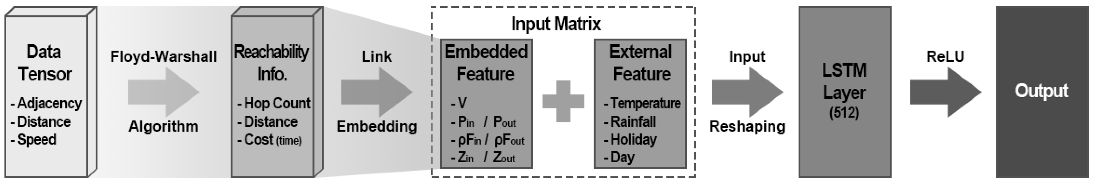
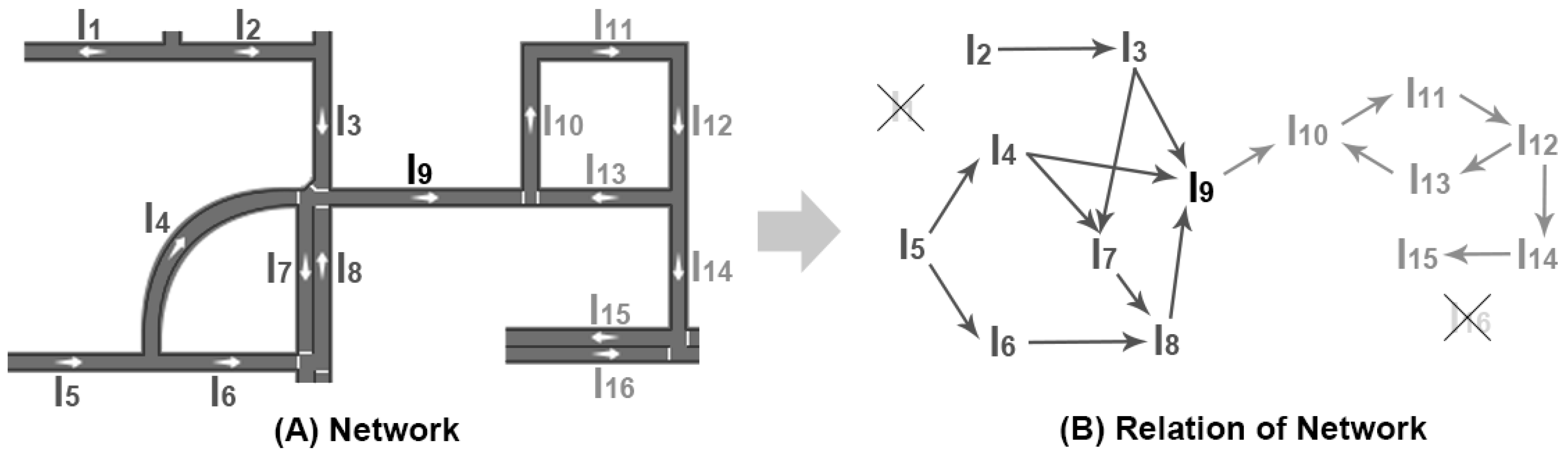
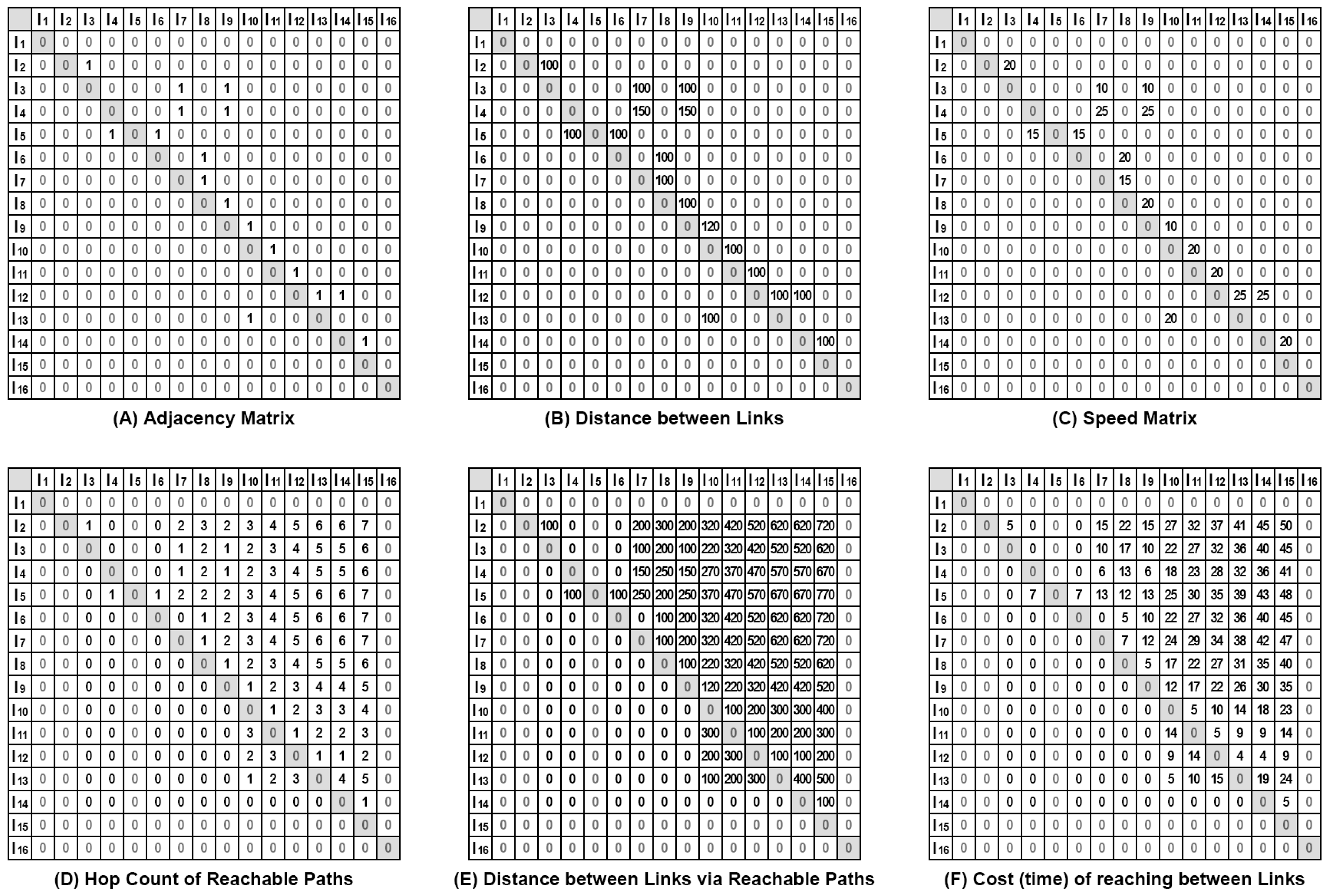
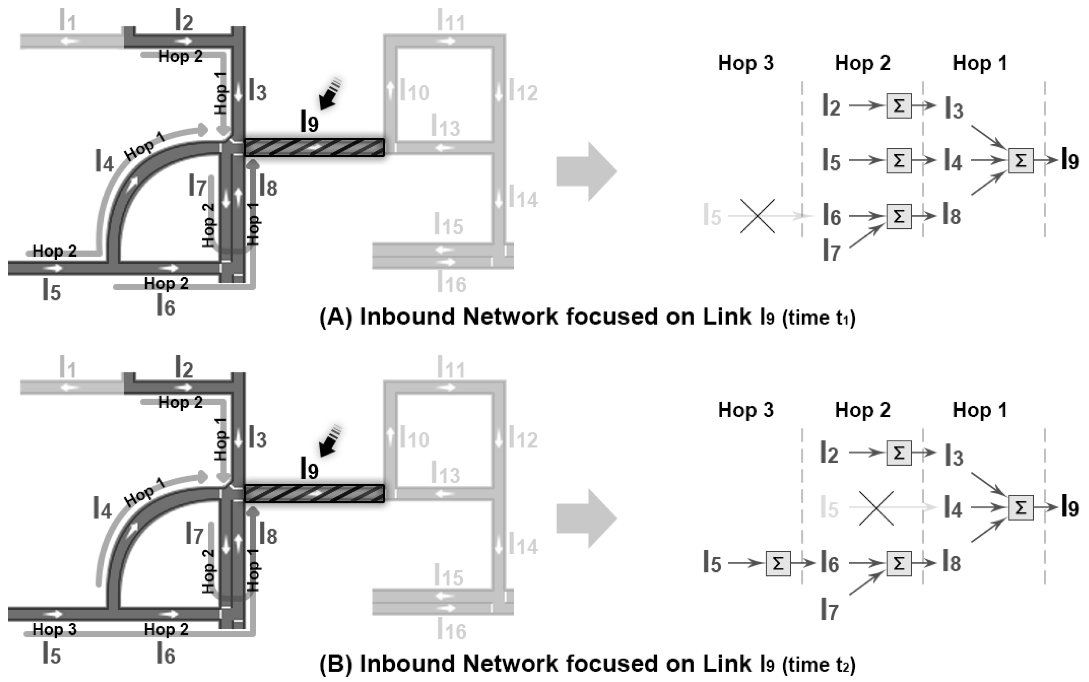
3.1. Link Embedding
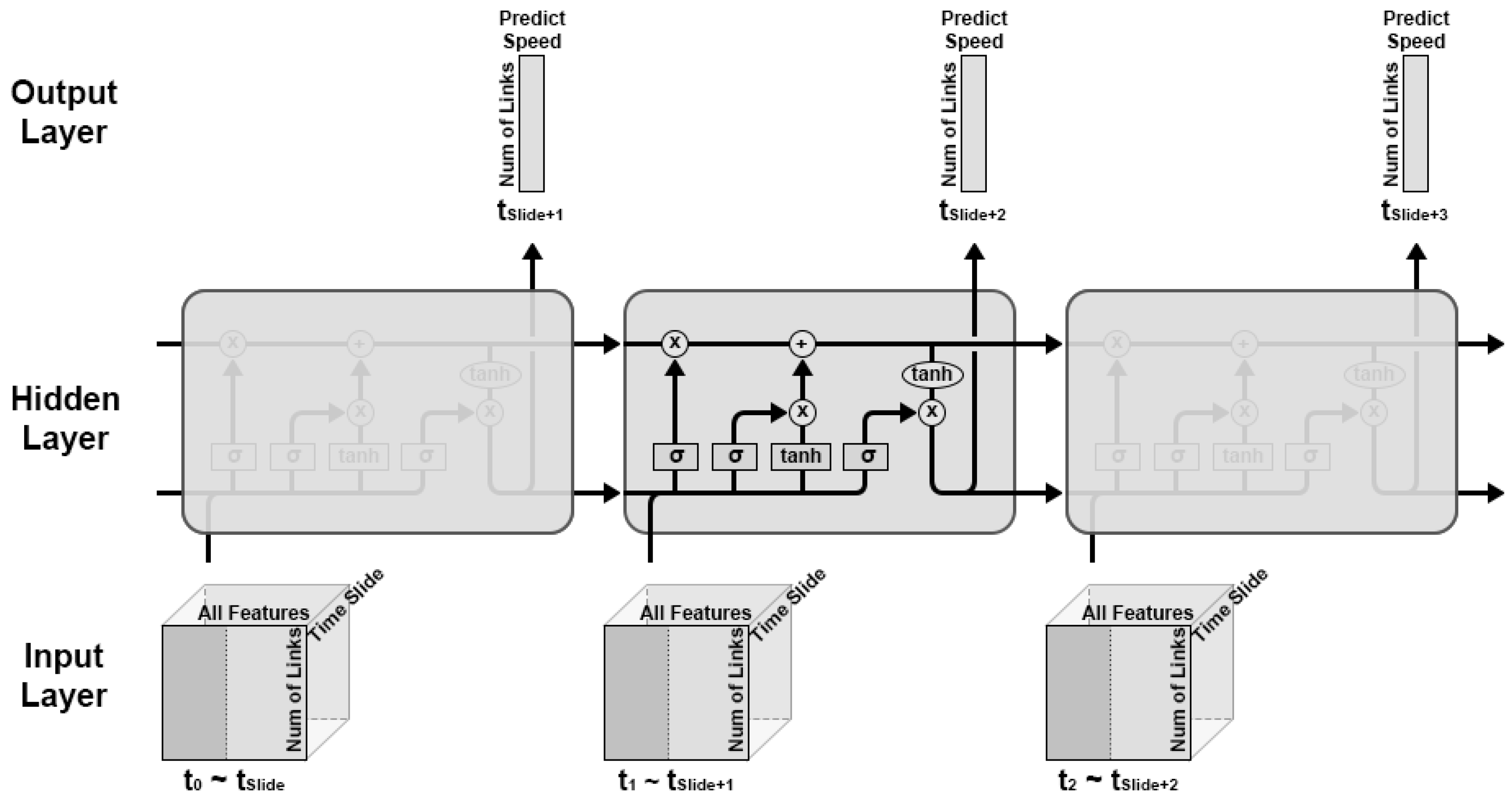
3.2. Modeling the Temporal Patterns with Recurrent Neural Networks
4. Evaluation
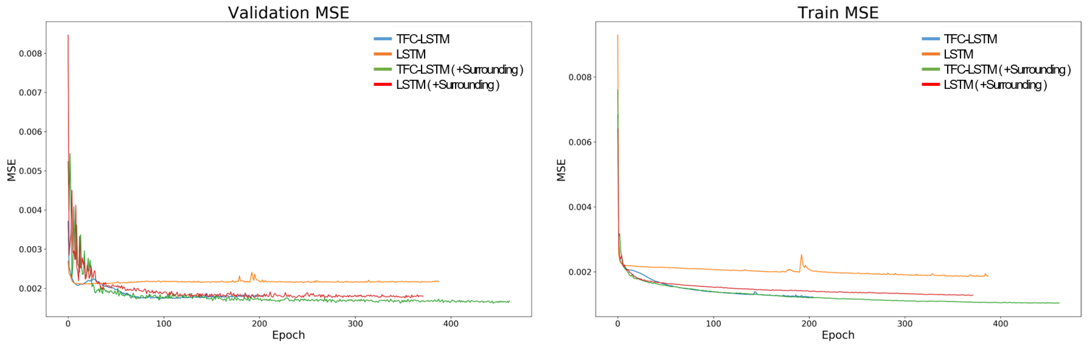
4.1. Measurement of Prediction Performance
4.2. The Effect of Reachable Path Length Cutoff
4.3. The Discussion on Scalability
5. Conclusions
Author Contributions
Funding
Conflicts of Interest
Abbreviations
| OD | Origin and Destination |
| TFC | Traffic Flow Centrality (Z value) |
References
- Williams, B.M.; Hoel, L.A. Modeling and Forecasting Vehicular Traffic Flow as a Seasonal ARIMA Process: Theoretical Basis and Empirical Results. J. Transp. Eng. 2003, 129, 664–672. [Google Scholar] [CrossRef]
- Kumar, S.V.; Vanajakshi, L. Short-Term Traffic Flow Prediction using Seasonal ARIMA Model with Limited Input Data. Eur. Transp. Res. Rev. 2015, 7, 21. [Google Scholar] [CrossRef]
- Chen, C.; Hu, J.; Meng, Q.; Zhang, Y. Short-Time Traffic Flow Prediction with ARIMA-GARCH Model. In Proceedings of the 2011 IEEE Intelligent Vehicles Symposium (IV), Baden-Baden, Germany, 5–9 June 2011; pp. 607–612. [Google Scholar]
- Jeong, Y.S.; Byon, Y.J.; Castro-Neto, M.M.; Easa, S.M. Supervised Weighting-Online Learning Algorithm for Short-Term Traffic Flow Prediction. IEEE Trans. Intell. Transp. Syst. 2013, 14, 1700–1707. [Google Scholar] [CrossRef]
- Wu, C.H.; Ho, J.M.; Lee, D.T. Travel-Time Prediction with Support Vector Regression. IEEE Trans. Intell. Transp. Syst. 2004, 5, 276–281. [Google Scholar] [CrossRef]
- Cai, P.; Wang, Y.; Lu, G.; Chen, P.; Ding, C.; Sun, J. A Spatiotemporal Correlative K-Nearest Neighbor Model for Short-Term Traffic Multistep Forecasting. Transp. Res. Part C Emerg. Technol. 2016, 62, 21–34. [Google Scholar] [CrossRef]
- Kim, T.; Kim, H.; Lovell, D.J. Traffic Flow Forecasting: Overcoming Memoryless Property in Nearest Neighbor Non-Parametric Regression. In Proceedings of the 2005 IEEE Intelligent Transportation Systems, Vienna, Austria, 16 September 2005; pp. 965–969. [Google Scholar]
- Yin, H.; Wong, S.; Xu, J.; Wong, C. Urban Traffic Flow Prediction using a Fuzzy-Neural Approach. Transp. Res. Part C Emerg. Technol. 2002, 10, 85–98. [Google Scholar] [CrossRef]
- Quek, C.; Pasquier, M.; Lim, B.B.S. POP-TRAFFIC: A Novel Fuzzy Neural Approach to Road Traffic Analysis and Prediction. IEEE Trans. Intell. Transp. Syst. 2006, 7, 133–146. [Google Scholar] [CrossRef]
- Guo, S.; Lin, Y.; Li, S.; Chen, Z.; Wan, H. Deep Spatial-Temporal 3D Convolutional Neural Networks for Traffic Data Forecasting. IEEE Trans. Intell. Transp. Syst. 2019, 20, 3913–3926. [Google Scholar] [CrossRef]
- Lv, Y.; Duan, Y.; Kang, W.; Li, Z.; Wang, F.Y. Traffic Flow Prediction with Big Data: A Deep Learning Approach. IEEE Trans. Intell. Transp. Syst. 2014, 16, 865–873. [Google Scholar] [CrossRef]
- Koesdwiady, A.; Soua, R.; Karray, F. Improving Traffic Flow Prediction with Weather Information in Connected Cars: A Deep Learning Approach. IEEE Trans. Veh. Technol. 2016, 65, 9508–9517. [Google Scholar] [CrossRef]
- Tian, Y.; Pan, L. Predicting Short-Term Traffic Flow by Long Short-Term Memory Recurrent Neural Network. In Proceedings of the 2015 IEEE International Conference on Smart City/SocialCom/SustainCom (SmartCity), Chengdu, China, 19–21 December 2015; pp. 153–158. [Google Scholar]
- Fu, R.; Zhang, Z.; Li, L. Using LSTM and GRU Neural Network Methods for Traffic Flow Prediction. In Proceedings of the 2016 31st Youth Academic Annual Conference of Chinese Association of Automation (YAC), Wuhan, China, 11–13 November 2016; pp. 324–328. [Google Scholar]
- Huang, W.; Song, G.; Hong, H.; Xie, K. Deep Architecture for Traffic Flow Prediction: Deep Belief Networks with Multitask Learning. IEEE Trans. Intell. Transp. Syst. 2014, 15, 2191–2201. [Google Scholar] [CrossRef]
- Du, B.; Peng, H.; Wang, S.; Bhuiyan, M.Z.A.; Wang, L.; Gong, Q.; Liu, L.; Li, J. Deep Irregular Convolutional Residual LSTM for Urban Traffic Passenger Flows Prediction. IEEE Trans. Intell. Transp. Syst. 2019, 21, 972–985. [Google Scholar] [CrossRef]
- Gu, Y.; Lu, W.; Xu, X.; Qin, L.; Shao, Z.; Zhang, H. An Improved Bayesian Combination Model for Short-Term Traffic Prediction with Deep Learning. IEEE Trans. Intell. Transp. Syst. 2019, 21, 1332–1342. [Google Scholar] [CrossRef]
- Cui, Z.; Henrickson, K.; Ke, R.; Wang, Y. Traffic Graph Convolutional Recurrent Neural Network: A Deep Learning Framework for Network-Scale Traffic Learning and Forecasting. IEEE Trans. Intell. Transp. Syst. 2019. [Google Scholar] [CrossRef]
- Hamilton, W.L.; Ying, R.; Leskovec, J. Representation Learning on Graphs: Methods and Applications. arXiv 2017, arXiv:1709.05584. [Google Scholar]
- Floyd, R.W. Algorithm 97: Shortest Path. Commun. ACM 1962, 5, 345. [Google Scholar] [CrossRef]
- Zhang, J.; Zheng, Y.; Qi, D.; Li, R.; Yi, X. DNN-based Prediction Model for Spatio-temporal Data. In Proceedings of the 24th ACM SIGSPATIAL International Conference on Advances in Geographic Information Systems, Burlingame, CA, USA, 31 October–3 November 2016; pp. 1–4. [Google Scholar]
- Kim, D.H.; Hwang, K.Y.; Yoon, Y. Prediction of Traffic Congestion in Seoul by Deep Neural Network. J. Korea Inst. Intell. Transp. Syst. 2019, 18, 44–57. [Google Scholar] [CrossRef]
- Zheng, Z.; Yang, Y.; Liu, J.; Dai, H.N.; Zhang, Y. Deep and Embedded Learning Approach for Traffic Flow Prediction in Urban Informatics. IEEE Trans. Intell. Transp. Syst. 2019, 20, 3927–3939. [Google Scholar] [CrossRef]
- Sun, S.; Wu, H.; Xiang, L. City-wide traffic flow forecasting using a deep convolutional neural network. Sensors 2020, 20, 421. [Google Scholar] [CrossRef]
- Hochreiter, S.; Schmidhuber, J. Long Short-Term Memory. Neural Comput. 1997, 9, 1735–1780. [Google Scholar] [CrossRef]
- Krizhevsky, A.; Sutskever, I.; Hinton, G.E. Imagenet Classification with Deep Convolutional Neural Networks. In Proceedings of the Advances in Neural Information Processing Systems, Lake Tahoe, NV, USA, 3–6 December 2012; pp. 1097–1105. [Google Scholar]
- Karpathy, A.; Toderici, G.; Shetty, S.; Leung, T.; Sukthankar, R.; Li, F.-F. Large-Scale Video Classification with Convolutional Neural Networks. In Proceedings of the IEEE conference on Computer Vision and Pattern Recognition, Columbus, OH, USA, 23–28 June 2014; pp. 1725–1732. [Google Scholar]
- Ji, S.; Xu, W.; Yang, M.; Yu, K. 3D Convolutional Neural Networks for Human Action Recognition. IEEE Trans. Pattern Anal. Mach. Intell. 2012, 35, 221–231. [Google Scholar] [CrossRef]
- Chung, J.; Gulcehre, C.; Cho, K.; Bengio, Y. Empirical Evaluation of Gated Recurrent Neural Networks on Sequence Modeling. arXiv 2014, arXiv:1412.3555. [Google Scholar]
- Jia, Y.; Wu, J.; Xu, M. Traffic Flow Prediction with Rainfall Impact using a Deep Learning Method. J. Adv. Transp. 2017, 2017. [Google Scholar] [CrossRef]
- Yu, B.; Lee, Y.; Sohn, K. Forecasting Road Traffic Speeds by Considering Area-Wide Spatio-temporal Dependencies based on a Graph Convolutional Neural Network (GCN). Transp. Res. Part C Emerg. Technol. 2020, 114, 189–204. [Google Scholar] [CrossRef]
- Ge, L.; Li, S.; Wang, Y.; Chang, F.; Wu, K. Global Spatial-Temporal Graph Convolutional Network for Urban Traffic Speed Prediction. Appl. Sci. 2020, 10, 1509. [Google Scholar] [CrossRef]
- Lu, H.; Huang, D.; Song, Y.; Jiang, D.; Zhou, T.; Qin, J. St-trafficnet: A spatial-temporal deep learning network for traffic forecasting. Electronics 2020, 9, 1474. [Google Scholar] [CrossRef]
- Scarselli, F.; Gori, M.; Tsoi, A.C.; Hagenbuchner, M.; Monfardini, G. The Graph Neural Network Model. IEEE Trans. Neural Netw. 2008, 20, 61–80. [Google Scholar] [CrossRef]
- Kipf, T.N.; Welling, M. Semi-Supervised Classification with Graph Convolutional Networks. arXiv 2016, arXiv:1609.02907. [Google Scholar]
- Nair, V.; Hinton, G.E. Rectified Linear Units Improve Restricted Boltzmann Machines. In Proceedings of the 27th International Conference on Machine Learning (ICML 2010), Haifa, Israel, 21–24 June 2010. [Google Scholar]
- Glorot, X.; Bordes, A.; Bengio, Y. Deep Sparse Rectifier Neural Networks. In Proceedings of the Fourteenth International Conference on Artificial Intelligence and Statistics, Fort Lauderdale, FL, USA, 11–13 April 2011; pp. 315–323. [Google Scholar]
- Kingma, D.P.; Ba, J. Adam: A method for Stochastic Optimization. arXiv 2014, arXiv:1412.6980. [Google Scholar]
- Ruder, S. An Overview of Gradient Descent Optimization Algorithms. arXiv 2016, arXiv:1609.04747. [Google Scholar]
- Yu, B.; Yin, H.; Zhu, Z. Spatio-temporal Graph Convolutional Networks: A Deep Learning Framework for Traffic Forecasting. arXiv 2017, arXiv:1709.04875. [Google Scholar]
- Zhao, L.; Song, Y.; Zhang, C.; Liu, Y.; Wang, P.; Lin, T.; Deng, M.; Li, H. T-GCN: A Temporal Graph Convolutional Network for Traffic Prediction. IEEE Trans. Intell. Transp. Syst. 2019, 21, 3848–3858. [Google Scholar] [CrossRef]


| Prediction Models | Raw Data Usage | Traffic Network Representation | |||||
|---|---|---|---|---|---|---|---|
| Traffic Speed/Volume | Traffic Network Structure | Surrounding Conditions | Invariant Input Feature Vector Size | Traffic Flow Reachability Analysis | Centrality Analysis | Chains of Neighbors | |
| TFC-LSTM | O | O | O | O | O | O | O |
| TGC-LSTM [18] | O | O | X | X | X | X | X |
| ST-3DNET [10] | O | O | X | X | X | X | X |
| DST-ICRL [16] | O | O | O | X | X | X | X |
| IBCM-DL [17] | O | X | X | X | X | X | X |
| DBN [15] | O | X | X | X | X | X | X |
| LSTM [13] | O | X | X | X | X | X | X |
| GRU [14] | O | X | X | X | X | X | X |
| DNN [12,22] | O | X | O | X | X | X | X |
| FNN [8,9] | O | O | X | X | X | O | X |
| K-NN [6,7] | O | O | X | X | O | X | X |
| SVR [4,5] | O | O | X | X | X | X | X |
| ARIMA [1,2,3] | O | X | X | X | X | X | X |
| Data | Speed | Temperature | Precipitation | Day | Holiday |
|---|---|---|---|---|---|
| Mean | 28.17 | 12.88 | 0.14 | - | - |
| Median | 25.62 | 13.7 | 0 | - | - |
| Max | 110.00 | 40.5 | 76 | 1 | 1 |
| Min | 0.74 | −27.1 | 0 | 0 | 0 |
| Unit | km/h | °C | mm | - | - |
| Time Interval | 1 h | 1 h | 1 h | 1 day | 1 day |
| Type | float | float | float | binary | binary |
| Epsilon | MAE | RMSE | MAPE |
|---|---|---|---|
| 0.1 | 2.60 | 4.40 | 10.84 |
| 0.05 | 2.69 | 4.48 | 11.16 |
| 0.01 | 2.63 | 4.41 | 11.07 |
| 0.005 | 2.50 | 4.28 | 10.39 |
| 0.001 | 2.69 | 4.43 | 11.15 |
| 0.0005 | 2.59 | 4.36 | 10.79 |
| 0.0001 | 2.54 | 4.32 | 10.51 |
| Prediction Models | Usage of Surrounding | Hidden Layer Structure | # of Time | MAE | RMSE | MAPE |
|---|---|---|---|---|---|---|
| Condition Information | (# of Perceptrons per Layer) | Windows | ||||
| DNN [12,22] | No | Double layers (64-8) | - | 4.05 | 6.25 | 15.58 |
| Yes | Double layers (64-8) | - | 4.36 | 6.42 | 17.36 | |
| TFC-DNN | No | Double layers (64-8) | - | 3.84 | 5.98 | 15.27 |
| Yes | Double layers (64-8) | - | 3.96 | 6.01 | 17.02 | |
| GRU [14] | No | Single layer (512) | 18 | 3.70 | 5.51 | 14.42 |
| Yes | Single Layer (512) | 18 | 7.52 | 10.20 | 31.12 | |
| TFC-GRU | No | Single layer (512) | 18 | 2.85 | 4.60 | 11.42 |
| Yes | Single Layer (512) | 18 | 6.20 | 8.12 | 22.57 | |
| LSTM [13] | No | Single layer (512) | 18 | 2.88 | 4.91 | 11.89 |
| Yes | Single Layer (512) | 18 | 2.64 | 4.48 | 10.87 | |
| TFC-LSTM | No | Single layer (512) | 18 | 2.63 | 4.47 | 11.38 |
| Yes | Single layer (512) | 18 | 2.50 | 4.28 | 10.39 |
| Lowest Speed Period | Highest Speed Period | MAE | RMSE | MAPE |
|---|---|---|---|---|
| 15 hops | 15 hops | 2.61 | 4.38 | 10.83 |
| 30 hops | 30 hops | 2.51 | 4.30 | 10.48 |
| 45 hops | 45 hops | 2.61 | 4.40 | 10.96 |
| 15 hops | 45 hops | 2.50 | 4.28 | 10.39 |
| 45 hops | 15 hops | 2.63 | 4.44 | 10.98 |
Publisher’s Note: MDPI stays neutral with regard to jurisdictional claims in published maps and institutional affiliations. |
© 2020 by the authors. Licensee MDPI, Basel, Switzerland. This article is an open access article distributed under the terms and conditions of the Creative Commons Attribution (CC BY) license (http://creativecommons.org/licenses/by/4.0/).
Share and Cite
Lee, C.; Yoon, Y. Context-Aware Link Embedding with Reachability and Flow Centrality Analysis for Accurate Speed Prediction for Large-Scale Traffic Networks. Electronics 2020, 9, 1800. https://doi.org/10.3390/electronics9111800
Lee C, Yoon Y. Context-Aware Link Embedding with Reachability and Flow Centrality Analysis for Accurate Speed Prediction for Large-Scale Traffic Networks. Electronics. 2020; 9(11):1800. https://doi.org/10.3390/electronics9111800
Chicago/Turabian StyleLee, Chanjae, and Young Yoon. 2020. "Context-Aware Link Embedding with Reachability and Flow Centrality Analysis for Accurate Speed Prediction for Large-Scale Traffic Networks" Electronics 9, no. 11: 1800. https://doi.org/10.3390/electronics9111800
APA StyleLee, C., & Yoon, Y. (2020). Context-Aware Link Embedding with Reachability and Flow Centrality Analysis for Accurate Speed Prediction for Large-Scale Traffic Networks. Electronics, 9(11), 1800. https://doi.org/10.3390/electronics9111800