Deep Learning of Appearance Affinity for Multi-Object Tracking and Re-Identification: A Comparative View

Abstract

Recognizing the identity of a query individual in a surveillance sequence is the core of Multi-Object Tracking (MOT) and Re-Identification (Re-Id) algorithms. Both tasks can be addressed by measuring the appearance affinity between people observations with a deep neural model. Nevertheless, the differences in their specifications and, consequently, in the characteristics and constraints of the available training data for each one of these tasks, arise from the necessity of employing different learning approaches to attain each one of them. This article offers a comparative view of the Double-Margin-Contrastive and the Triplet loss function, and analyzes the benefits and drawbacks of applying each one of them to learn an Appearance Affinity model for Tracking and Re-Identification. A batch of experiments have been conducted, and their results support the hypothesis concluded from the presented study: Triplet loss function is more effective than the Contrastive one when an Re-Id model is learnt, and, conversely, in the MOT domain, the Contrastive loss can better discriminate between pairs of images rendering the same person or not.

1. Introduction

In the 21st century, security awareness has deeply changed. This is the result of the evolving global situation and the increasing threat of a wide variety of types of crime, such as robbery, theft, burglary and inter-personal crime, like bullying, harassment, and assault, and even terrorism and cross border intrusions. One of the immediate reactions to these threats and citizens’ concerns is the growing implantation of video surveillance systems, in public and private places. This results in the expansion of the surveillance market across the world [1].

Manual video-surveillance by a human operator is an inefficient solution, due to the high manpower costs, operators’ limited capacity to monitor a certain number of screens or the limited attention span [2]. Consequently, Intelligent Surveillance Systems (ISS) [3,4] are emerging to automatically monitor the environment with less (second generation) [5], or without human intervention (third generation). These ISS aim to monitor a determinate environment in real-time, providing an automatic interpretation of the scene and predicting the individuals’ actions and interactions, based on the data acquired by sensors.

The current research trend seeks to increase the wideness of the monitored areas, as well as the robustness and scalability of the surveillance systems using the design of distributed architectures [6], like in PRISMATICA [7] and ADVISOR [8] projects. In distributed surveillance systems, every camera works as a non-centralized and relatively autonomous entity, which interacts with the others in a dynamic environment, leading to a network, where each cooperative sensor employs artificial vision methods, besides the data from the neighboring devices [9].

These distributed systems state the necessity of efficient algorithms to perform the tracking of multiple individuals through video streams from multiple and distant camera views, known as Multi-Target Multi-Camera Tracking (MTMCT). The automatisation of MTMCT is essential to enable some applications including suspicious activity and anomaly detection, and crowd behavior analysis in a distributed surveillance system.

In turn, MTMCT is composed of two types of computer vision algorithms: Multi-Object Tracking (MOT) and Person Re-Identification (Re-Id) algorithms. Multi-Object Tracking consists of finding the position of multiple people from their visual measurements and conserving their identities in a video sequence from a certain monitoring point. Person Re-Identification consists of visually recognizing an individual across non-overlapping camera views at different and distant locations and time, which is necessary to extend the functionalities of an ISS through several camera views.

In the literature, the tracking automatisation is commonly solved under the “tracking-by-detection” paradigm, e.g.,  [10,11]. Once a set of people detections is collected, the tracker performs a data association task, where the detections at every new frame are assigned to their corresponding tracked identities. The data association process is mainly composed of an optimization method for seeking the identities assignment that minimizes the matching cost. In turn, the cost of matching a detection with a certain identity is computed by a metric that compares the features rendering both the current detections and the previous tracks.

In the past decades, important research progress has been made in solving the data association problem [12,13,14]. However, the final tracking performance is limited by the design of the person representation and the cost function. Some of the most commonly used features are related to individuals’ motion, such as location or velocity, [15,16,17], and even the interactions between agents, with social force models, e.g.,  [18,19] and crowd motion pattern models [20,21].

Nevertheless, the presence of frequent individuals’ occlusions and interactions, in unconstrained and crowded scenarios, makes the use of algorithms relying only on motion cues insufficient, which boosts the research on modeling individuals’ appearance. Therefore, a primary task in people tracking is converting raw pixels into higher-level representations. Many objects trackers, like [22], rely on extracting appearance information from the object pixels using hand-crafted features, including appearance information via a color histogram [23,24,25] and texture descriptors [23,26,27], which are the most popular representation for appearance modeling in MOT.

Recently, deep neural network architectures have been used for modeling appearance [28,29,30]. In these architectures, high-level features are extracted by Deep Convolutional Neural Networks (DCNN).

Some tracking algorithms get improvements by modeling every tracked person independently, e.g., [31,32]. These dedicated models are trained online since there is no previous knowledge about the individuals to track. The drawback of these approaches is that a certain time is needed until the online learning catches enough number of samples of a person to learn a reliable pattern. For that reason, in many association methods, models to compare two observations are learnt. These works explicitly learn affinity metrics from data. Therefore, the pairwise terms, which connect two observations, can be weighted by offline trained appearance templates or a simple distance metric between appearance features, as in the network-flow-based methods proposed in [14,33], respectively. In contrast, in [34], a simple fixed appearance model is incorporated into a standard Multi Hypotheses Tracking framework. Then, Leal-Taix’e et al. [29] trained a Siamese neural network to compare the appearance of two detections and combine this with spatial and temporal differences in a boosting framework.

Similarly to the recent trends in MOT development, the research in person Re-Identification has been also mainly focused on developing visual appearance-based methods. The reason is that, usually, in real-world surveillance scenarios, temporal and spatial constraints are difficult to establish, since cameras are often placed far apart and their fields of view do not always overlap, and fine bio-metric cues cannot be acquired from distant sensors.

Concretely, the objective in Single Shot Re-Identification task is to match the person appearing in an image (probe), with its corresponding representation among a set of images captured from a different view (gallery). Single-Shot Re-Id allows for reducing the quantity of data transmitted between neighbors’ cameras, compared with Multi-Shot Re-Id, which relies on the previous tracking of a person to obtain a tracklet formed by consecutive detections. Therefore, Single-Shot Re-Id speed up communications in a distributed network of cooperative surveillance sensors. Hence, in Single-Shot Re-Id, the comparison of two images must provide a prediction of whether they belong to the same identity or not. A pair of images of the same person is hereinafter called a matched or positive pair. Analogously, a pair of images of different people is denoted as a mismatched or negative pair.

Therefore, similarly to the data association in MOT, the Person Re-Identification problem can be treated as a pairwise binary classification task, composed of two main components: features extraction and the learning of their optimal combination to discriminate positive and negative pairs.

Consequently, earlier methods for Re-Id generally fall into two categories. Firstly, approaches focused on enhancing the person features designs to represent the most discriminant aspects of an individual’s appearance, e.g.,  [35,36,37]. Then, other methods were meant to learn an effective discriminative distance to optimally combine the previously extracted visual features, e.g.,  [38,39,40,41].

Recently, there are some works of literature applying neural models to address the Re-Id problem. These approaches follow a supervised learning framework, [42], whose overall network architecture is a Siamese network with two branches or a Triplet model with three branches.

The first two works in Re-Id to use deep learning, [43,44], employed a Siamese neural network to model the similarity between a pair of images. Indeed, the Siamese network had been earlier used to verify signatures [45]. Siamese Networks consist of two DCNN branches, sharing parameters and joined in the last layer, where the loss function performs a pairwise verification [44,46,47,48]. Each branch computes the feature representation for one of the images of a pair. The distance between the learnt features measures the affinity between the images. Hence, the objective is to make the distances for positive pairs smaller than that for negative ones, achieving a binary classification in the distance space.

Traditionally, Siamese networks have been trained through the Contrastive Loss function, proposed in [49]. This function forces the distance between matched pairs of images to be lower than a set margin, and higher for mismatched pairs. Then, in [50], a double-margin-based version of the Contrastive loss was presented. This function, hereinafter called Double-Margin Contrastive loss, forces the distances between matched pairs to be lower than a first margin, and the distances between negative pairs to be larger than a second margin. This formulation increases the discriminative capacity of the learnt features by keeping a distance gap between the classes.

Then, another widely used loss to train contrastive models the Triplet loss. The basics of the Triplet loss computation are presented in [51], where face recognition is addressed. This function is employed to automatically find salient high-level features from raw images, like in the works presented in [52,53]. In the Triplet model, each training input is a set of three samples, instead of two. Two of the three images are rendering the same person and the third one, a different identity. Hence, the triplet model compares a matched and a mismatched pair from each triplet input, so the objective function can maximize the relative distance between them.

For that reason, some works [54,55] extend the triplet approach to the Re-Id problem with an efficient learning algorithm and a triplet generation scheme. Wang et al. [54] proposed a model which involved learning features for fine-grained image retrieval. They pre-trained the neural network designed by Krizhevsky et al. [56], using soft-max loss function, but they did not clarify whether their triplet model can be effective without pre-training techniques. Then, Ding et al. [55] demonstrated the effectiveness of their model using a relatively simple network without pre-training techniques.

Many works build each branch of the triplet model with neural architectures that were previously designed for different purposes, like the VGG (Visual Geometry Group) architectures, introduced in [57], by Oxford’s Visual Geometry Group. For instance, Zhuang et al. [53] chose the VGG16 model to learnt representative features to solve Face Re-Identification with a triplet model, and Liu et al. [58] to address Person Re-Identification.

In conclusion, the research on both MOT and Re-Id methods has been recently focused on applying neural models to measure the appearance affinity between different detections. This approach has been boosted by the success of Deep Convolutional Neural Networks to automatically find salient high-level features from the pixels of an image in various vision problems, such as image classification [57,59], objects detection [60], or face identification [61].

However, although deep learning has been proven to provide successful results in many fields of application, its potential to learn a unique appearance model, able to represent any anonymous individual in a scene, has not been sufficiently exploited yet and brings an assortment of new learning challenges.

The recognition of a certain identity using a neural model presents an intrinsically unbalanced nature, given the shortage of data about the individuals to identify and the vast number of possible false associations with surrounding agents. This results in the over-fitting and collapse of the neural models used to render the visual appearance.

This article assumes that both Multi-Person Tracking and Re-Identification can be similarly addressed by the learning of appearance affinity models. Indeed, a model to measure the Appearance Affinity between an image and a set of possible candidates has been trained for Person Re-Identification. Such a neural model has also been trained for measuring the matching score between two observations in a data association mechanism for Multi-Object Tracking.

Given the unpredictable nature of the video surveillance task in unstructured scenarios, MOT and Re-Id algorithms must be versatile to deal with any unknown individual. To achieve this, the idea of independently modeling any of the appearing individuals’ appearance has been discarded. Instead of this, a universal model has been designed to measure the Appearance Affinity between two person images. This model predicts whether the images correspond to the same person or not.

Furthermore, this article performs a study of the effects of the data constraints on the learning of person features through contrastive neural architectures. A unique DCNN model (base network) has been to learnt and combine person features for both surveillance tasks, MOT and Re-id. Nevertheless, the differences in the data constraints presented for each task results in the necessity of using a specialized learning strategy to train the DCNN network for each purpose. For that reason, this article presents a comparative analysis of the benefits of choosing the Double-Margin Contrastive loss or the Triplet loss for learning person features to address MOT or Re-Id problem, whilst keeping the same base network architecture, concretely a VGG network. The main contributions of this work are:

• Implementation of a neural model to measure the Appearance Affinity between observations for addressing both, the MOT, and the Re-Id problem.
• Study of the differences in data constraints derived from the specifications of each task, MOT, and Re-Id.
• Formulation and implementation of mini-batch learning algorithms to train a base network (concretely with a VGG architecture) under the Siamese and the Triplet model.
• Comparative analysis of the effects of imposing the Double-Margin-Contrastive Loss and the Triplet Loss constrains over the MOT and the Re-Id data.

A batch of experiments has been conducted and their meaningful results have been thoroughly analyzed to extract useful conclusions and guidelines about the learning of affinity models from MOT or Re-Id data.

The rest of the article is structured as follows: the Section 2 presents the architecture of the affinity model to train, the comparative study of the MOT and the Re-Id tasks and the implemented learning algorithm. Section 3 describes the conducted experiments and their results. Section 4 analyzes and discusses the obtained results, and, finally, Section 5 gives some concluding remarks.

2. Appearance Affinity Learning

To exploit the visual appearance of a target individual to track and re-identify him/her among multiple people, a model of Appearance Affinity has been developed.

The measurement of the Appearance Affinity has been formulated as a pairwise binary classification problem, which consists of the computation of features for a pair of person images and its comparison through a distance metric, as Figure 1 shows. Consequently, an input pair formed by images of the same person is considered as a positive pair, and a pair consisting of images of different people is taken as a negative pair. Hence, instead of modeling a specific individual’s appearance pattern, the situations of similarity and dissimilarity are discriminated in two classes.

Due to the contrastive essence of this pairwise approach, the measured distance can be understood as the probability of a pair of images belonging to the dissimilarity class. In addition, the complementary probability, as their Appearance Affinity.

Instead of computing the distances directly over the raw images, these are calculated from some feature embeddings. Therefore, it is necessary to model a feature function, $F\left(I\right)$, to map an input image, I, to a feature space, such that the distances between samples rendering the same person are smaller than those between different people in that feature space. This feature embedding has been modeled by a DCNN. Therefore, the feature representation for an image, I, is given by the output of the DCNN, $F_W\left(I\right)$, which relies on its weights values, W.

2.1. Base Neural Network

The transformation of every image, I, to its corresponding representation in the feature space, $F_W\left(I\right)$, has been performed by a DCNN with a well-known architecture. Concretely, a version of the architecture presented as the A version of a set of Very Deep CNN in [57]. This is a 11-layered network, hereafter called VGG11. The architecture VGG16 has been widely used to implement face recognition models, e.g.,  [53]. However, the initial experiments conducted with re-identification data demonstrated that the architecture VGG11 provide slightly better performance since it reduces the model over-fitting thanks to the lower number of parameters to train. The layers specifications for the proposed VGG11-based embedding are listed in

Table 1. Structure of the used VGG11-based model. The input and output sizes are described in $\#rows$ × $\#cols$ × $\#filters$; the kernel, in $\#rows$ × $\#cols$ × $\#filters$, $stride$, or $\#out puts$ for FC layers.

Layer	Input Size	Output Size	Kernel
Conv-1-1	128 × 64 × 3	128 × 64 × 64	3 × 3 × 3
Pool-1	128 × 64 × 64	64 × 32 × 64	2 × 2 × 64, 2
Conv-2-1	64 × 32 × 64	64 × 32 × 128	3 × 3 × 64
Pool-2	64 × 32 × 128	32 × 16 × 128	2 × 2 × 128, 2
Conv-3-1	32 × 16 × 128	32 × 16 × 256	3 × 3 × 128
Conv-3-2	32 × 16 × 256	32 × 16 × 256	3 × 3 × 256
Pool-3	32 × 16 × 256	16 × 8 × 256	2 × 2 × 256, 2
Conv-4-1	16 × 8 × 256	16 × 8 × 512	3 × 3 × 256
Conv-4-2	16 × 8 × 512	16 × 8 × 512	3 × 3 × 512
Pool-4	16 × 8 × 512	8 × 4 × 512	2 × 2 × 512, 2
Conv-5-1	8 × 4 × 512	8 × 4 × 512	3 × 3 × 512
Conv-5-2	8 × 4 × 512	8 × 4 × 512	3 × 3 × 512
Pool-5	8 × 4 × 512	4 × 2 × 512	2 × 2 × 512, 2
FC-6	4 × 2 × 512	1 × 1 × 4096	4096
FC-7	1 × 1 × 4096	1 × 1 × 4096	4096
FC-8	1 × 1 × 4096	1 × 1 × 1000	1000

.

The original VGG11 presents eight convolution layers, three fully connected layers, and a SoftMax final layer. The SoftMax layer has been removed to get a feature array as output, instead of a classification probability value. Hence, its output is a point in a 1000-dimensional feature space, $F\left(I\right)\in {\mathbb{R}}^n$ ($n=1000$). Furthermore, the original input size has been modified to adapt its value to the dimensions of the people detections in surveillance sequences. The input size has been standardized. Therefore, the input of the proposed DCNN is an RGB image of 64 × 128 pixels, which is a common size in Re-Id datasets. All hidden layers use the ReLU activation function [56].

2.2. Analysis of Multi-Object Tracking and Re-Identification Challenges: Differences on Data

There are differences in the limitations and the characteristics of the training data for MOT and Re-Id. These differences are the consequence of the specifications of each target task:

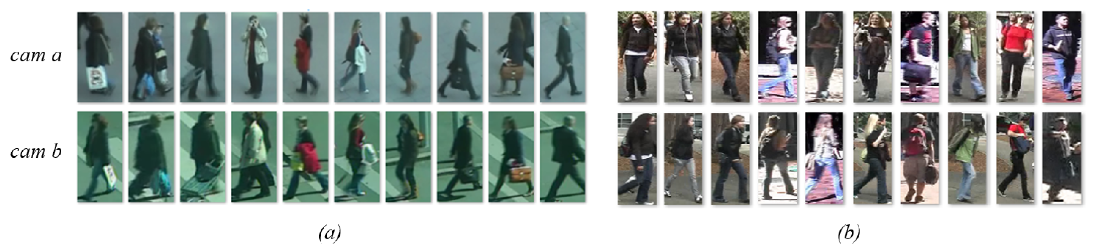
• Camera view. In an MOT system, the identification of a certain individual is performed through a video sequence that is captured from a certain camera. Therefore, the compared observations of the query person are captured from the same monitoring point. On contrary, by definition, Person Re-identification is the recognition of an individual across images that are captured from different and non-overlapping camera views. This results in extended periods of occlusion and large changes of viewpoint and illumination across different fields of view.
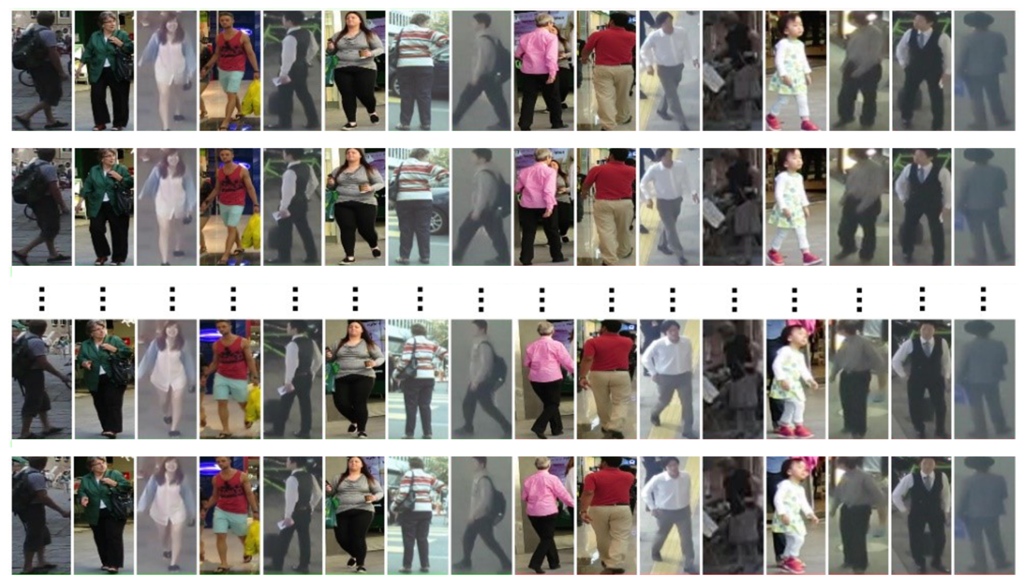
• Number of samples of each individual. In a Single-Shot Re-Identification system, identity recognition is performed from only two images of every individual, one per camera view. However, in a tracking sequence, there are so many samples of a person as frames where the person appears.

The exposed differences in the tasks specifications results in a number of particular characteristics of the available data for each task, which are listed as follows:

• Intra-class variations. In the Re-Id frame, intra-class variations are caused by the significant and unknown cross-view feature distortion between two different capturing points. The differences between the camera characteristics and point of view of two different monitoring points cause large changes in perspective, illumination, background, pose, scale, and resolution. This results in dramatically different appearances and consequently different representations of the same person. In MOT sequences, every detection of an individual is captured from the same device, so the intra-class variation is smaller. However, the data can also present certain appearance variations due to temporal occlusions, the presence of fast-moving people or the use of moving camera platforms, which vary the pose, illumination, and background between observations.
• Inter-class ambiguity. Inter-class ambiguities are produced by the existence of different individuals with almost identical shape and wearing similar clothes and hairstyles. These ambiguities are more accused in Re-Id data, where the representation of a person is compared with that across view variations, so it can be more similar to the representation of another person than himself/herself.
• Local features alignment. The variations of viewpoints and poses cause misalignment in the compared human shapes. These misalignments are caused by occlusions and moving cameras in MOT domain, and by the different location of the camera views in Re-Id domain, where the variations are more pronounced.
• Binary classification balance. The number of samples of a query individual is very reduced, specifically when compared with the huge amount of potentially available detections of different people. The Single-Shot Re-Identification task is especially affected by the unbalanced nature of its underlying data (two samples per person). In an MOT system, the number of samples of a certain individual is equal to the number of frames where the query person has appeared, which is reduced when new individuals enter in the field of view of the surveillance camera.

The consequence of these differences in the data characteristics is that the distribution of the MOT training data in a prior feature space differs from that of the Re-Id data, as Figure 2 shows. In Figure 2, a simple bidimensional feature space is rendered to exemplify the general trends in data distribution, where each color point renders a sample from a certain identity. The smaller intra-class variations and inter-class ambiguities in MOT data allow a clearer clustering of the samples of a certain individual in the feature space. Moreover, the number of samples in each identity cluster is much higher than that in Re-Id data, where there are only two images per person.

The objective of the affinity model is to measure a distance metric, $dm$, between a pair of samples and discriminate whether the pair is positive (images of the same person) or negative (images of different people). The distance between the features measures dissimilarity between the images so the objective is to get smaller distances for positive pairs than for negative ones, achieving a binary classification in the distance space. Nevertheless, the high intra-class variations and inter-class ambiguities in the data are translated to a notable sparsity of the data in the distance metric space. This effect hampers the discrimination in two classes, especially in Re-Id data, as Figure 3 shows.

A model meant to perform a certain task must be trained on data with a similar distribution to the target data with which the model is supposed to deal. Therefore, the differences in the specifications of the MOT and Re-Id data call for the training of the proposed affinity model on two different training set types: those generated from Re-Id shots, and those, from MOT sequences. Both types of training sets have been generated by a data combination tool (The data generation tool is a set of C++ functions, which are publicly available under http://github.com/magomezs/dataset_factory.)

The Re-Id training sets have been generated by forming positive and negative pairs of images from two Single-Shot Re-Id datasets: PRID2011 [62] and VIPeR [63], which are described in detail in Section 3.1. In both datasets, only one image per person and per view is given. Figure 4 shows examples of matched pairs (in each column) from these datasets. Every pair is formed by images that were captured from two different cameras views (cam a and cam b).

The MOT training sets have been generated by extracting and combining people detections from the MOT17 dataset. This dataset includes fourteen variate real-world surveillance sequences. Seven of these sequences provide their MOT ground truth with the bounding boxes of the people detections in every frame and their identification numbers. All the detections of every individual throughout each sequence have been extracted thanks to the ground truth information, as Figure 5 shows. Subsequently, positive and negative pairs have been generated from the extracted samples. The samples composing a positive pair do not have to be consecutive in time, but a certain time step between the frames from which they come has been allowed. The negative pairs can be formed by detections from different sequences of the MOT17 dataset.

The differences between each type of training set arise the necessity of employing different loss functions, and, consequently, the implementation of adapted learning algorithms, as the following subsection describes.

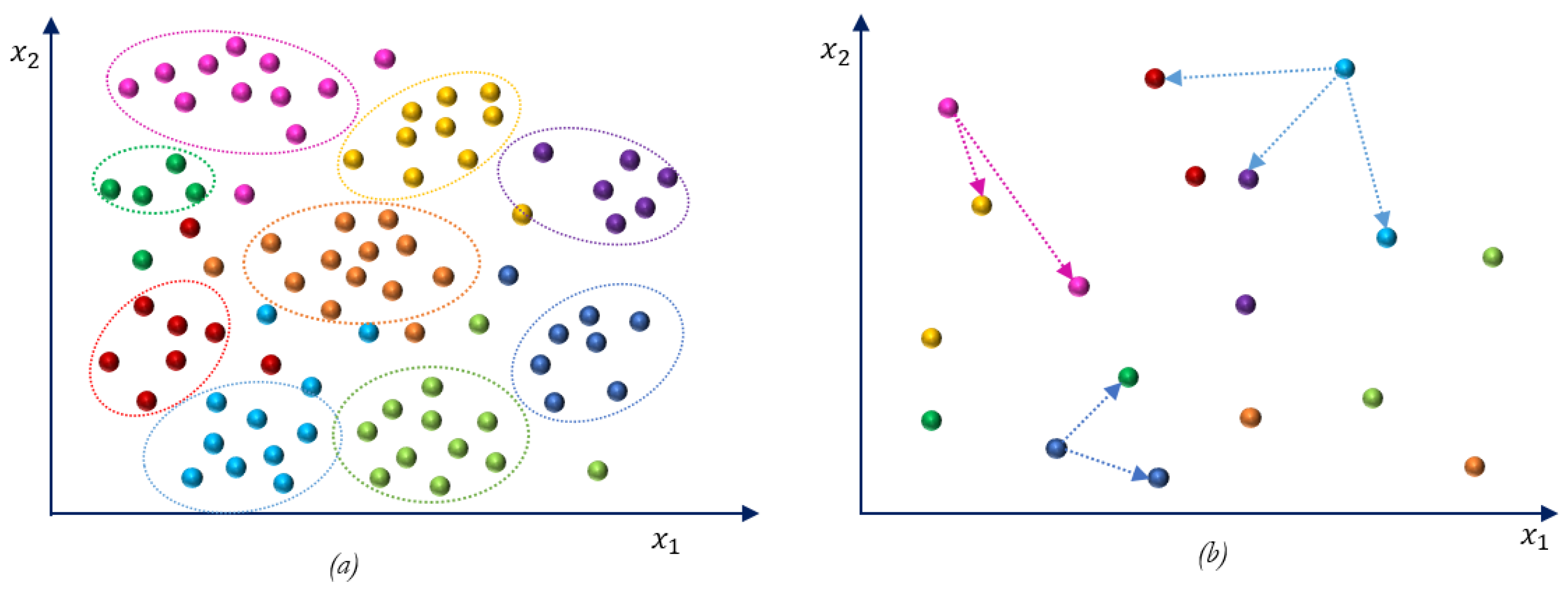
2.3. Double-Margin-Contrastive Loss vs. Triplet Loss

To compute the proposed Appearance Affinity metric, a feature embedding, $F\left(I\right)$, has to be previously modeled by a DCNN. The general aim is to learn a transformation from the raw image to the feature space, such it leads the representations for the same person near, and far away from different people’s representations. The weights of this DCNN are trained to minimize a certain loss function which mathematically defines the sought objective. Therefore, the chosen loss function determines the learning process evolution, its convergence, and the discriminative capacity of the finally learnt feature embedding.

The Double-Margin-Contrastive loss function (The Double-Margin-Contrastive loss function is implemented in a Caffe python layer, which is publicly available under http://github.com/magomezs/N2M-Contrastive-Loss-Layer), $f_{2MCL}$, presented in [50], is based on two margins to establish the separation between the objective values of the metric distances for positive and negative samples. The traditional Contrastive Loss function, presented in [49], was based in only one margin. In comparison, the result of using two margins is an increment in the discriminative capacity of the learnt features, since positive and negative pairs move away from each other in the feature space. Both classes of pairs, positive and negative ones, are not simply separated by one boundary value (one margin) in the distance space, but by a gap defined by two fixed boundaries (two margins). Therefore, the Double-Margin-Contrastive loss function reduces the inter-class ambiguities.

The formulation of the Double-Margin-Contrastive loss function is described by Equation (1) for a batch of B pairs. This function measures the half average of the error computed for every pair, with respect to the constant margins, $m_1$ and $m_2$. $NDM(nd{m}_1,\dots ,nd{m}_B)$ is an array, where every element, $nd{m}_i$, is the normalized distance metric for one of the pairs of the treated batch in one learning iteration. That means that, for every sample i of the batch, the distance metric, $dm$, is previously normalized by Equation (2), where e is Euler’s number. In turn, the distance metric, $dm$, is computed by the squared Euclidean distance between the features of the query pair sample $X_i=\langle I^a,I^b\rangle$, as Equation (3) defines. Finally, Y is an array, where every element, $y_i$, is the value given by the labeler function for the pair i. The labeler function, $y(I^a,I^b)$, takes value 1 for positive pairs, and 0, for negative ones, according to Equation (4):

$$f_{2MCL}(NDM,Y)=\frac{1}{2B}\sum _{i=1}^B[y_i·max(nd{m}_i-m_1,0)+(1-y_i)·max(m_2-nd{m}_i,0)]$$

(1)

$$ndm=2\left(\frac{1}{1+e^{-dm}}-0.5\right)$$

(2)

$$dm\left(X_i\right)={\parallel F_W\left(I_i^a\right)-F_W\left(I_i^b\right)\parallel }_2^2$$

(3)

$$y(I^a,I^b)=\left\{\begin{array}{cc}1& \mathrm{i}\mathrm{f} ID\left(I^a\right)=ID\left(I^b\right)\\ 0& \mathrm{i}\mathrm{f} ID\left(I^a\right)\ne ID\left(I^b\right)\end{array}\right.$$

(4)

Therefore, an effective training process leads the $ndm$ to be lower than $m_1$ for positive samples and higher than $m_2$ for negative ones. According to Equation (1), positive samples with a distance value lower than the first margin, $m_1$, and negative samples with a distance higher than the second margin, $m_2$ do not cause any loss value. The setting of the margins depends on the range of values presented by the distances, $dm$. Nevertheless, this range varies along the training process. For that reason, the distances are normalized within the range of values $[0,1)$. Eventually, the margin parameters have been set with the values $m_1=0.3$ and $m_2=0.7$.

Meanwhile, the Triplet loss function, presented in [51], establishes a relative distance relationship. Every i sample of the training dataset, X, is constituted by a triplet of person images, $X_i=\langle I_i^a,I_i^p,I_i^n\rangle$, where $I_i^a$ is an anchor image, $I_i^p$ renders the same person than the anchor image, and $I_i^n$ is a different person’s image. Therefore, $I_i^a$ and $I_i^p$ form a positive pair of samples, and they present the same identification number. The identification number of $I_i^n$ is different, so the pair formed by this image and the anchor image, $I_i^a$, is a negative pair. The triplet model tries to maximize the relative distance between the distance metric values for the positive and the negative pair. A batch formulation of the Triplet loss, $f_{TL}$, is defined by Equation (5), where B is the number of elements in a batch of triplets, $X^t=X_i$. For a certain triplet of images, the triplet loss requires the squared Euclidean distance for the negative pair to be larger than that for the positive one by a predefined margin, $\tau$:

$$f_{TL}\left(W^t;X^t\right)=\frac{1}{2B}\sum _{i=1}^B\left[max\right(\tau +\parallel F_w\left(I_i^a\right)-F_w\left(I_i^p\right){\parallel }_2^2-\parallel F_w\left(I_i^a\right)-F_w\left(I_i^n\right){\parallel }_2^2,0\left)\right]$$

(5)

To fairly compare the performance of the Double-Margin-Contrastive loss and the Triplet one. The parameter, $\tau$ has been set with value 0.4, which is the difference between the chosen margins values for the Contrastive loss.

Both loss functions can be used to train a binary pair-wise classifier, like the proposed Appearance Affinity model. Nevertheless, there exist differences between their formulations that affect the learning of the model.

Even though the magnitude of the margin used by the Triplet loss function is constant, the extreme boundaries separating the classes are not. The distance between positive and negative pairs is relative. Conversely, the Contrastive loss function classifies positives and negatives pairs in an independent way, without considering the relative distance between positive and negative instances of a given identity. Therefore, the fixed boundaries (margins) separating similarity and dissimilarity classes are fixed on the Double-Margin-Contrastive loss function, as Figure 6 renders.

The relative essence of the comparison made by the triplet loss function makes it flexible and adaptative to deal with the situation of different people with similar appearance, which produces small values of the distance for negative pairs, and the occurrence of high distance values for positive pairs due to quite different representations of the same individual (see Figure 3). In the presence of the mentioned situations, which are quite common in Re-Identification, in contrast to the triplet loss, the contrastive loss value is prone to suffer from strong oscillations and slow convergence.

The Double-Margin-Contrastive loss function cannot compare positive and negative samples between them. Instead of that, positive and negative samples are independently compared with fixed boundaries, and these constraints could be too demanding in the first learning iterations. However, the smaller intra-class variation and inter-class ambiguity among the people detections from tracking sequences make the application of the Contrastive loss in the MOT domain suitable. In the MOT frame, the discriminative capacity of the Double-Margin-Contrastive loss can be exploited without falling in the convergence problem of a too demanding objective function, since, a priori, the MOT data are easier to cluster than the Re-Id data, as Figure 2 shows.

2.4. Learning Algorithm Implementation

The selection of the Double-Margin-Contrastive loss function or the Triplet one determines the general architecture of the learning model and the formulation of the employed learning algorithm. The use of the Contrastive function translates into a Siamese configuration, where the DCNN to train is duplicated. Analogously, the Triplet loss calls for a triplet architecture, where the DCNN is triplicated. Therefore, in the Siamese model, every training input is composed of a pair of images, while in the Triplet model, of a triplet of them. Two versions of the Mini-batch Gradient Descent algorithm have been implemented, each one of them adapted to a type of input data, pairs or triplets. In both models, the DCNN branches are forced to share the same weights. This means that the learnt weights, W, are identical in all the branches, so a unique feature embedding is learnt.

The two branches of the Siamese model are joined in the final layers, where the affinity is measured, by comparing the obtained features with a distance metric, as Figure 7 shows.

The input of the Siamese model is a pair of images, $I^a$ and $I^b$, where the indexes a and b refer to the branch receiving each image. The order of the inputs can be commuted without effects on the result. Moreover, each image is accompanied by an identification number, $ID\left(I\right)$, since a supervised trained has been conducted.

The descriptor defined by the DCNN is computed twice (once per image) in the forward propagation of the network. Once the person features for an input pair of images, $(F_W\left(I^a\right),F_W\left(I^b\right))$, have been computed, they must be compared by the squared Euclidean distance to get the distance metric, $dm$.

Finally, in the last layer, the loss function measures the deviation of the computed distance value with respect to the established objective values for positive ($y=1$) and negative pairs ($y=0$). Therefore, in every iteration, the loss value measures how the classification made by the forward propagation of the network differs from the correct one, given by the label y. The loss value is consequently used by the back-propagation method [64] to force the weights in both branches to get values which make the distance metric, $dm$, get closer to the objective. For that reason, the loss function plays a crucial role in the learning process.

Instead of duplicating the DCNN in two branches, as the Siamese model does, Triplet model triplicates it, as Figure 8 shows. The first branch of the triplet model receives an anchor sample, $I_i^a$, the second one takes an image, $I_i^p$, rendering the same person than the anchor image, and the input of the third branch is a different person’s image, $I_i^n$. The triplet model tries to maximize the relative distance between the distance metric values for the positive, $d{m}_{+}$ and the negative pair, $d{m}_{-}$.

A feature descriptor is computed for every input by the forward propagation of the DCNN. The affinity between the anchor images, $I_i^a$, and the positive and negative inputs, $I_i^p$, $I_i^n$, is measured by computing the squared Euclidean distance between the features arrays of the images, $F_W\left(I_i^a\right)$, $F_W\left(I_i^p\right)$, $F_W\left(I_i^n\right)$. Then, the distances are contrasted by the Triplet Loss function.

In both domains, MOT and Re-Id, the available quantity of data about each individual is very poor in comparison with the huge amount of possible different identities in a scene. Although this lack of data are more accused in Re-Id task, in general, the available data are not enough to adopt an individual-meant training approach, which clusters the same person samples close from each other and distant to another person identity cluster. By contrast, the proposed affinity model treats all the possible positive pairs as a set rendering the condition of similarity. Analogously, negative pairs represent the dissimilarity situation.

The discrimination between similarity and dissimilarity has been learnt using comparing every positive pair with all the possible negative pairs. In that way, the network is trained to be able to identify a person between a huge number of negative samples. This global comparison approach calls for the use of a Batch learning algorithm. However, the huge amount of possible pairs and triplet combinations composing the training set, and the limitations in processing memory resources, have led to implementing a Mini-Batch learning algorithm. In the performed training processes, the chosen batch size was that as large as the available memory resources make possible ($B=128$ in the Siamese learning, and $B=64$ in the Triplet learning).

A Pair and a Triplet version of the Mini-Batch Gradient Descent learning algorithm have been implemented to train the VGG network over MOT and Re-Id data. Their main procedures are shown by Algorithms 1 and 2, respectively.

Algorithm 1 Pair-based Mini-Batch Gradient Descent Learning Algorithm.

Require: Batches of pairs, $X^t=\left\{X_i^t\right\}$. Ensure: The network parameters $W^T=\left\{W_j^T\right\}$.  $W^0=\left\{W_j^0\right\}$ 2: while t < T do     $t\leftarrow t+1$; 4:     $\frac{\partial f_{2MCL}\left(W^t,X^t\right)}{\partial W_j^t}=0$;     for all training pair $X_i^t=(I^a,I^b)$ of the batch set $X^t$ do 6:         Calculate $F_{W^t}\left(I^a\right)$, and $F_{W^t}\left(I^b\right)$ by forward propagation;         Calculate $nd{m}_i$ by Equations (2) and (3); 8:     end for     Calculate $f_{2MCL}\left(W^t,X^t\right)$ by Equation (1); 10:     for all training pair $X_i^t=(I^a,I^b)$ of the batch set $X^t$ do         Calculate $\frac{\partial nd{m}_i}{\partial W_j^t}$, by Equation (9); 12:         Calculate $\frac{\partial F_{W^t}\left(I^a\right)}{\partial W_j^t}$, and $\frac{\partial F_{W^t}\left(I^b\right)}{\partial W_j^t}$, by back propagation;     end for 14:     Calculate $\frac{\partial f_{2MCL}(W^t;X^t)}{\partial W_j^t}$ according to Equations (10) and (11);     Update parameters according to Adagrad method [65]; 16: end while

Algorithm 1 computes the features of each pair of images from the training batch by forward propagation, and the distance between them, $ndm$ by Equations (2) and (3). Then, the value of the loss function $f_{2MCL}$ is obtained with Equation (1).

Subsequently, the back-propagation of the two neural branches is performed to obtain $\frac{\partial F_{W^t}\left(I^a\right)}{\partial W_j^t}$, and $\frac{\partial F_{W^t}\left(I^b\right)}{\partial W_j^t}$ for every sample of the batch. From these derivatives, the distance derivative, $\frac{\partial ndm}{\partial W_j^t}$, is computed, using Equation (9). This equation is the result of defining $\frac{\partial ndm}{\partial W_j^t}$ as Equation (6), and substituting each term by its formulation, given by Equations (7) and (8) and by the definition of $dm$, Equation (3). The term given by $\frac{\partial ndm}{\partial dm}$ has been obviated in practice since this is a factor bounded between 0 and $0.5$. Thus, it has a similar effect as the learning rate, $\alpha$, whose value is properly adapted by the Adagrad method, [65]. In addition, this factor does not affect the gradient descent direction, and its estimation is computationally expensive.

Finally, the partial derivatives of the Double-Margin-Contrastive loss function, with respect to the set of learnt weights, $W=\left\{W_j\right\}$, are defined by Equations (10) and (11). Then, both processes, forward and back-propagation, are repeated until achieving the pre-established maximum number of iterations, T:

$$\frac{\partial ndm}{\partial W_j^t}=\frac{\partial ndm}{\partial dm}·\frac{\partial dm}{\partial W_j^t}$$

(6)

$$\frac{\partial ndm}{\partial dm}=\frac{2e^{-dm}}{{(e^{-dm}+1)}^2}=\frac{2e^{-{\parallel F_W\left(I_i^a\right)-F_W\left(I_i^b\right)\parallel }_2^2}}{{(e^{-{\parallel F_W\left(I_i^a\right)-F_W\left(I_i^b\right)\parallel }_2^2}+1)}^2}$$

(7)

$$\frac{\partial dm}{\partial W_j^t}=\frac{\partial dm}{\partial F_W\left(I_i^a\right)}·\frac{\partial F_W\left(I_i^a\right)}{\partial W_j^t}+\frac{\partial dm}{\partial F_W\left(I_i^b\right)}·\frac{\partial F_W\left(I_i^b\right)}{\partial W_j^t}=2·\left(F_W\left(I_i^a\right)·\frac{\partial F_W\left(I_i^a\right)}{\partial W_j^t}-F_W\left(I_i^b\right)·\frac{\partial F_W\left(I_i^b\right)}{\partial W_j^t}\right)$$

(8)

$$\frac{\partial ndm}{\partial W_j^t}=\frac{2e^{-{\parallel F_W\left(I_i^a\right)-F_W\left(I_i^b\right)\parallel }_2^2}}{{(e^{-{\parallel F_W\left(I_i^a\right)-F_W\left(I_i^b\right)\parallel }_2^2}+1)}^2}·2·\left(F_W\left(I_i^a\right)·\frac{\partial F_W\left(I_i^a\right)}{\partial W_j^t}-F_W\left(I_i^b\right)·\frac{\partial F_W\left(I_i^b\right)}{\partial W_j^t}\right)$$

(9)

$$\frac{\partial f_{2MCL}}{\partial W_j}=\frac{1}{2B}\sum _{i=1}^B{h}_1$$

(10)

$$h_1=\left\{\begin{array}{cc}\frac{\partial nd{m}_i}{\partial W_j}& \mathrm{i}\mathrm{f} y_i=1\wedge nd{m}_i>m_1\\ -\frac{\partial nd{m}_i}{\partial W_j}& \mathrm{i}\mathrm{f} y_i=0\wedge nd{m}_i<m_2\\ 0& \mathrm{o}\mathrm{t}\mathrm{h}\mathrm{e}\mathrm{r}\mathrm{w}\mathrm{i}\mathrm{s}\mathrm{e}\end{array}\right.$$

(11)

Analogously, Algorithm 2 computes the features of each triplet of images from the training batch by forward propagation, to get the value of the loss function, $f_{TL}$ with Equation (5). Then, the partial derivatives of the loss function, given a set of learnt weights, $W=\left\{W_j\right\}$, defined by Equations (12) and (13), are computed using Equations (14)–(16).

The back-propagation of the three neural branches is performed to obtain $\frac{\partial F_{W^t}\left(I^a\right)}{\partial W_j^t}$, $\frac{\partial F_{W^t}\left(I^p\right)}{\partial W_j^t}$ and $\frac{\partial F_{W^t}\left(I^n\right)}{\partial W_j^t}$ for every sample of the batch. Both processes, forward and back-propagation, are repeated until achieving the pre-established maximum number of iterations, T.

In the experiments where the network was trained over MOT data, the model weights W were initialized using the Xavier method [66]. However, when the training data came from Re-Id datasets, to alleviate the Re-Id data problem, the network weights, $W^0=\left\{w_j^0\right\}$, were initialized with values that were pre-trained on MOT domain as is detailed in [67].

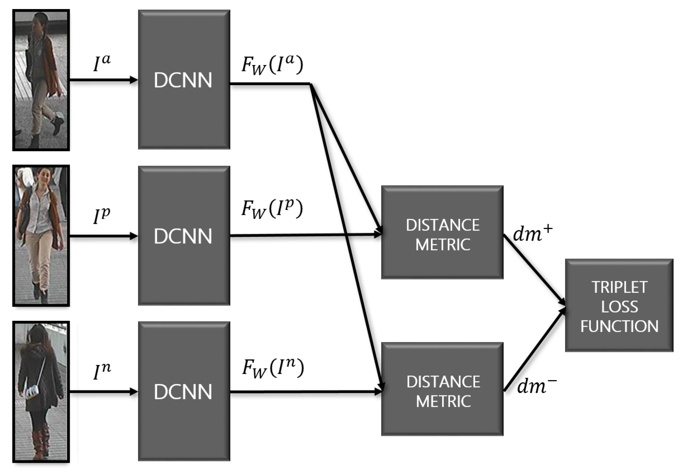
Algorithm 2 Triplet-based Mini-Batch Gradient Descent Learning Algorithm [67].

Require: Batches of triplets, $X^t=\left\{X_i^t\right\}$. Ensure: The network parameters $W^T=\left\{W_j^T\right\}$. 1: $W^0=\left\{W_j^0\right\}$ 2: while t < T do 3:     $t\leftarrow t+1$; 4:     $\frac{\partial f_{TL}\left(W^t,X^t\right)}{\partial W_j^t}=0$; 5:     for all training triplet $X_i^t=(I^a,I^p,I^n)$ of the batch set $X^t$ do 6:         Calculate $F_{W^t}\left(I^a\right)$, $F_{W^t}\left(I^p\right)$ and $F_{W^t}\left(I^n\right)$ by forward propagation; 7:     end for 8:     Calculate $f_L\left(W^t;X^t\right)$ by Equation (5); 9:     for all training triplet $X_i^t=(I^a,I^p,I^n)$ of the batch set $X^t$ do 10:         Calculate $\frac{\partial f_C(W^t;X_i^t)}{\partial F_{W^t}\left(I^a\right)}$, $\frac{\partial f_C(W^t;X_i^t)}{\partial F_{W^t}\left(I^p\right)}$ and $\frac{\partial f_C(W^t;X_i^t)}{\partial F_{W^t}\left(I^n\right)}$ by Equations (14)–(16); 11:         Calculate $\frac{\partial F_{W^t}\left(I^a\right)}{\partial W_j^t}$, $\frac{\partial F_{W^t}\left(I^p\right)}{\partial W_j^t}$ and $\frac{\partial F_{W^t}\left(I^n\right)}{\partial W_j^t}$, by back propagation; 12:     end for 13:     Calculate $\frac{\partial f_L(W^t;X^t)}{\partial W_j^t}$ according to Equations (12) and (13); 14:     Update parameters according to the Adagrad method [65]; 15: end while

$$\frac{\partial f_L(W^t;X^t)}{\partial W_j^t}=\frac{1}{2B}\sum _{i=1}^B\left[\frac{\partial f_C(W^t;X_i^t)}{\partial W_j^t}\right]$$

(12)

$$\begin{array}{c}\hfill \frac{\partial f_C(W;X_i)}{\partial W_j}=\frac{\partial f_C(W;X_i)}{\partial F_W\left(I^a\right)}·\frac{\partial F_W\left(I^a\right)}{\partial W_j}+\frac{\partial f_C(W;X_i)}{\partial F_W\left(I^p\right)}·\frac{\partial F_W\left(I^p\right)}{\partial W_j}+\frac{\partial f_C(W;X_i)}{\partial F_W\left(I^n\right)}·\frac{\partial F_W\left(I^n\right)}{\partial W_j}\end{array}$$

(13)

$$\frac{\partial f_C(W;X_i)}{\partial F_W\left(I^a\right)}=\left\{\begin{array}{cc}2(F_W\left(I^n\right)-F_W\left(I^p\right))& if{dm}^{-}-d{m}^{+}<\tau \\ 0& otherwise\end{array}\right.$$

(14)

$$\frac{\partial f_C(W;X_i)}{\partial F_W\left(I^p\right)}=\left\{\begin{array}{cc}2\left(F_W\left(I^p\right)-F_W\left(I^a\right)\right)& if{dm}^{-}-{dm}^{+}<\tau \\ 0& otherwise\end{array}\right.$$

(15)

$$\frac{\partial f_C(W;X_i)}{\partial F_W\left(I^n\right)}=\left\{\begin{array}{cc}2\left(F_W\left(I^a\right)-F_W\left(I^n\right)\right)& if{dm}^{-}-{dm}^{+}<\tau \\ 0& otherwise\end{array}\right.$$

(16)

3. Results

The objective of this work is to demonstrate how the same DCNN (concretely, the VGG architecture) can be trained over MOT and Re-Id data using the Siamese and the Triplet model, and how the constraints imposed by Double-Margin-Contrastive loss and the Triplet loss are more or less appropriate to deal with the characteristics of the data distribution in each one of the mentioned domains: MOT and Re-Id.

This section evaluates not only the performance of the learnt models but also the effectiveness of the conducted learning processes. The next subsections describe the used target datasets, the metrics employed to evaluate the learnt affinity models, the conducted experiments and their results.

3.1. Datasets Protocol

The data from three bench-marked datasets have been taken to conduct experiments. One of them is a Multi-Object Tracking dataset, the MOT17 dataset. The other two datasets, PRID and VIPeR datasets, are Single-Shot Person Re-identification datasets.

• The MOT17 dataset belongs to the MOTchallenge (MOTChallenge is a Multiple Object Tracking Benchmark which provides a unified framework to standardise the evaluation of MOT methods. This is published under https://motchallenge.net/) and includes fourteen variate real-world surveillance sequences, meant to train and test Multi-Person Tracking algorithms, which were released in 2017. This benchmark contains challenging video sequences captured from static and moving cameras in unconstrained environments. The MOT17 dataset contains the same set of sequences as MOT16 [68], but with an extended more accurate ground truth. Seven of the sequences are accompanied by its corresponding ground-truth files and have been used to extract person images, to obtain samples of the identities appearing in those sequences.
• PRID2011 (PRID2011 dataset is publicly available under https://www.tugraz.at/institute/icg/research/team-bischof/lrs/downloads/prid11/) [69] is a Single-Shot Re-Id dataset that was captured from two different, static surveillance cameras, placed outdoors. This is composed of two sets of images, where all the images from one set, A, were captured from the same camera view, and all the samples from the other set, B, were acquired from a second camera view different from the first one. Set A contains 385 individuals and set B, 749. 200 of the captured individuals are rendered in both sets. In addition, 100 of them have been used to train the model. The test set has been formed by following the procedure described in [69], i.e., the images of set A for the 100 remaining individuals with representation in both sets have been used as the probe set. The gallery set has been formed by 649 images belonging to set B (all images of set B except the 100 corresponding to the training individuals).
• VIPeR (VIPeR dataset is publicly available under https://vision.soe.ucsc.edu/node/178) [63] is a Single-Shot Re-Id dataset where the images were captured from arbitrary viewpoints under varying illumination conditions, even inside the same set, but maintaining the assumption that the representation of a person in set A was captured from a different camera view than that from which its representation in the set B was captured. This dataset presents 632 pedestrians, each one with representation in both sets. For evaluation, the procedure described in [63] has been followed. The pairs have been randomly grouped into two sets of 316 pairs to train and test the model. Therefore, the gallery set is formed by 316 images from set A, and the probe set by their matching images from set B.

From each one of these datasets, a training set formed by positive and negative pairs has been generated by the method proposed in [70], where the difference between the number of possible positive and negative pairs is balanced until achieving a proportion of 1:4. These pair-based sets are used to train the Siamese model. Instead, the triplet model is fed by a training set formed by triplets that were created with the permutation method presented in [71].

3.2. Evaluation Methodology: Metrics

An appearance affinity model has been trained over MOT and Re-Id data with two different purposes: the first one is to measure the cost of associate an identity to a certain detection in the data association process of a tracking algorithm, and the second one is to obtain a model able to recognize an identity among a group of candidates, across different camera views. For that reason, the affinity models trained over MOT data have been evaluated as a binary classifier, to test their performance to discriminate between positive and negative pairs of samples. Instead of that, the ranking capacity of the models trained over Re-Id data has been measured. In both cases, the evaluation has been conducted over the samples of a test set, formed by pairs of images. Moreover, in particular, the training over Re-Id data are especially complicated due to the lack of training data, and, for that reason, the learning evolution has also been observed through the experiments.

• Evaluation of binary classification capacity. A ROC (Relative Operating Characteristic) [72] curve has been used to visualize the capacity of the learnt models to properly classify the pairs samples of the test set. This curve renders the diagnostic ability of a binary classifier as its discrimination threshold, $th$, is varied. $th$ defines the value until which the classifier output is considered as the prediction of a positive pair, and from which it is considered as a negative pair. The ROC curve plots the True Positive Rate ($TPR$), also called Sensitivity or Recall, against the False Positive Rate ($FPR$), also known as the fall-out rate. The $TPR$ and $FPR$ metrics are defined by Equations (17) and (18), respectively, where $TP$ is the number of true positives, $TN$ is the number of true negatives, $FP$ is the number of false positives, and $FN$ is the number of false negatives.

  $$TPR=\frac{TP}{TP+FN}$$

  (17)

  $$FPR=\frac{FP}{FP+TN}$$

  (18)
  Other metrics widely used to measure the performance of binary classifiers are Positive Predictive Value, $PPV$ (also called Precision), $F1$ score, and Accuracy, A, defined by Equations (19)–(21), respectively. $F1$ score provides a trade-off between precision and recall. The accuracy value, which is the proportion of well-classified pairs is not an appropriate metric for the case of having skewed classes In the case of identifying a person when he/she is compared with many people images, the ratio of positive samples to negative ones is very low. However, to provide a fair evaluation through the accuracy metric, the test set has been formed by the same number of positive as negatives pairs, presenting a completely balanced proportion of samples from each class.

  $$PPV=\frac{TP}{TP+FP}$$

  (19)

  $$F1=\frac{2·PPV·TPR}{PPV+TPR}$$

  (20)

  $$A=\frac{TP+TN}{TP+FP+TN+FN}$$

  (21)
• Evaluation of the Re-Id ranking capacity. The test set is formed by two groups of images, the set of probe images and the galley. The capacity of the model to rank the gallery images according to their affinity with a query probe image has been evaluated through the Cumulative Matching Characteristic (CMC) curve [73].
  To obtain the CMC curve, a query probe image is coupled with all the images from the gallery and the distance metrics, $dm$, between them are computed. The obtained distance metrics, $dm$, are ranked, and this process is repeated for each one of the probe images. The rank value, i.e., the position of the correct match in the rank, is calculated for each probe image and, subsequently, the percentage in which each rank appears. Then, the CMC curve renders the expectation of finding the correct match within the top r matches, for different values of r, called ranks. The computed percentages are cumulative.
  All the gallery images must be ranked in order of decreasing appearance affinity w.r.t. the probe image and the correct match must occupy the first position on the ranking. This is an extremely arduous task, since, even under the human criteria, the probe image can be visually more similar to gallery images from different people than to the corresponding one because of the inter-class ambiguities and the intra-class variations. Moreover, the person rendered in one probe image must be recognized among multiple gallery images. For instance, in PRID dataset, a probe individual must be found among 649 images. For that reason, CMC curves are not comparable to ROC curves, since the first ones represent the ranking capacity of a method instead of its classification capacity.
• Evaluation of the learning evolution. The evolution of every training process is evaluated by analyzing their learning curves, which is the representation of the loss function value throughout the learning process. This allows for checking the model convergence. The convergence of the Mini-Batch Gradient Descent cannot be guaranteed by an arithmetical method, but experimentally observing the progression of the learning curve of the training process. The Mini-Batch learning algorithm performs frequent parameters updates with a high variance that cause the objective function to fluctuate heavily, resulting in a learning curve with oscillations. Despite the oscillations, the convergence of the learning algorithms is proved by the decreasing tendency of their learning curves that eventually are stabilized around a certain value.

3.3. Experiments

Four experiments have been conducted. The presented base network has been trained and tested in each one of them. The differences among the experiments lie in the training data source, MOT or Re-Id databases, and in the chosen loss function, Double-Margin-Contrastive or Triplet, as

Table 2. Experiments settings.

Experiments	Description
	Data Source	Loss Function	Other Settings
Exp.MOT.Contrast	MOT domain	Double-Margin-Contrastive loss, $f_{2MCL}$, Equation (1)	VGG11 architecture. Euclidean distance metric. Adagrad optimizer. L2 regularization, $wd=0.0005$.
Exp.MOT.Triplet		Triplet loss, $f_{TL}$, Equation (5)
Exp.ReId.Contrast	Re-Id domain	Double-Margin-Contrastive loss, $f_{2MCL}$, Equation (1)
Exp.ReId.Triplet		Triplet loss, $f_{TL}$, Equation (5)

depicts. The loss function selection determines the training architecture, the training samples format and the learning algorithm. Therefore, Exp.MOT.Contrast and Exp.ReId.Contrast trained the base network with a Siamese architecture, feeding it with pairs of images, using Algorithm 1. Analogously, Exp.MOT.Triplet and Exp.MOT.Triplet learnt the features under a Triplet model, where the training inputs were triplets of images, employing Algorithm 2.

The visual appearance differences between a certain detection and its previously tracked observations can be successfully involved in their matching cost formulation. Through Exp.MOT.Contrasts and Exp.MOT.Triplet, the performance of the Contrastive and the Triplet loss functions to train an affinity model able to deal with MOT data have been compared. The results obtained with each one of them are presented by

Table 3. Binary classification metrics for the Appearance Affinity model learnt with the Double-Margin-Contrastive loss function.

$\mathit{th}$	$\mathit{TN}$	$\mathit{FN}$	$\mathit{FP}$	$\mathit{TP}$	$\mathit{TPR}$ [%]	$\mathit{FPR}$ [%]	$\mathit{PPV}$ [%]	${\mathit{F}}_1$ [%]	A [%]
$0.00$	$\mathrm{20,000}$	$\mathrm{20,000}$	0	0	0	0	-	-	$50.000$
$0.05$	$\mathrm{19,777}$	5758	223	$\mathrm{14,242}$	$71.21$	$3.73$	$98.46$	$82.646$	$85.048$
$0.10$	$\mathrm{19,441}$	3614	559	$\mathrm{16,386}$	$81.93$	$13.40$	$96.70$	$88.705$	$89.568$
$0.15$	$\mathrm{18,943}$	2498	1057	$\mathrm{17,502}$	$87.51$	$29.73$	$94.31$	$90.780$	$91.113$
$0.20$	$\mathrm{18,377}$	1702	1623	$\mathrm{18,298}$	$91.49$	$48.81$	$91.85$	$91.671$	$91.688$
$0.25$	$\mathrm{17,780}$	1106	2220	$\mathrm{18,894}$	$94.47$	$66.75$	$89.49$	$91.910$	$91.685$
$0.30$	$\mathrm{17,240}$	667	2760	$\mathrm{19,333}$	$96.67$	$80.54$	$87.51$	$91.859$	$91.433$
$0.35$	$\mathrm{16,771}$	378	3229	$\mathrm{19,622}$	$98.11$	$89.52$	$85.87$	$91.583$	$90.983$
$0.40$	$\mathrm{16,289}$	238	3711	$\mathrm{19,762}$	$98.81$	$93.97$	$84.19$	$90.916$	$90.128$
$0.45$	$\mathrm{15,774}$	149	4226	$\mathrm{19,851}$	$99.26$	$96.59$	$82.45$	$90.074$	$89.063$
$0.50$	$\mathrm{15,262}$	99	4738	$\mathrm{19,901}$	$99.51$	$97.95$	$80.77$	$89.164$	$87.908$
$0.55$	$\mathrm{14,648}$	59	5352	$\mathrm{19,941}$	$99.71$	$98.91$	$78.84$	$88.053$	$86.473$
$0.60$	$\mathrm{13,900}$	32	6100	$\mathrm{19,968}$	$99.84$	$99.48$	$76.60$	$86.689$	$84.670$
$0.65$	$\mathrm{13,150}$	16	6850	$\mathrm{19,984}$	$99.92$	$99.77$	$74.47$	$85.340$	$82.835$
$0.70$	$\mathrm{12,187}$	5	7813	$\mathrm{19,995}$	$99.98$	$99.94$	$71.90$	$83.647$	$80.455$
$0.75$	$\mathrm{11,213}$	0	8787	$\mathrm{20,000}$	$100.0$	$100.0$	$69.48$	$81.989$	$78.033$
$0.80$	9868	0	$\mathrm{10,132}$	$\mathrm{20,000}$	$100.0$	$100.0$	$66.38$	$79.789$	$74.670$
$0.85$	8498	0	$\mathrm{11,502}$	$\mathrm{20,000}$	$100.0$	$100.0$	$63.49$	$77.667$	$71.250$
$0.90$	7509	0	$\mathrm{12,491}$	$\mathrm{20,000}$	$100.0$	$100.0$	$61.56$	$76.204$	$68.773$
$0.95$	6047	0	$\mathrm{13,953}$	$\mathrm{20,000}$	$100.0$	$100.0$	$58.91$	$74.139$	$65.118$
$1.00$	0	0	$\mathrm{20,000}$	$\mathrm{20,000}$	$100.0$	$100.0$	$50.00$	$66.667$	$50.000$

and

Table 4. Binary classification metrics for the Appearance Affinity model learnt with the Triplet loss function.

$\mathit{th}$	$\mathit{TN}$	$\mathit{FN}$	$\mathit{FP}$	$\mathit{TP}$	$\mathit{TPR}$ [%]	$\mathit{FPR}$ [%]	$\mathit{PPV}$ [%]	${\mathit{F}}_1$ [%]	A [%]
$0.00$	20000	20000	0	0	0	0	-	-	$50.000$
$0.05$	$\mathrm{19,997}$	$\mathrm{14,727}$	3	5273	$26.37$	$0.02$	$99.94$	$41.723$	$63.175$
$0.10$	$\mathrm{19,990}$	$\mathrm{11,599}$	10	8401	$42.01$	$0.09$	$99.88$	$59.139$	$70.978$
$0.15$	$\mathrm{19,984}$	9516	16	$\mathrm{10,484}$	$52.42$	$0.17$	$99.85$	$68.748$	$76.170$
$0.20$	$\mathrm{19,970}$	7879	30	$\mathrm{12,121}$	$60.61$	$0.38$	$99.75$	$75.401$	$80.228$
$0.25$	$\mathrm{19,936}$	6542	64	$\mathrm{13,458}$	$67.29$	$0.97$	$99.53$	$80.294$	$83.485$
$0.30$	$\mathrm{19,878}$	5428	122	$\mathrm{14,572}$	$72.86$	$2.20$	$99.17$	$84.003$	$86.125$
$0.35$	$\mathrm{19,765}$	4540	235	$\mathrm{15,460}$	$77.30$	$4.92$	$98.50$	$86.623$	$88.063$
$0.40$	$\mathrm{19,600}$	3849	400	$\mathrm{16,151}$	$80.76$	$9.41$	$97.58$	$88.375$	$89.378$
$0.45$	$\mathrm{19,441}$	3370	559	$\mathrm{16,630}$	$83.15$	$14.23$	$96.75$	$89.435$	$90.178$
$0.50$	$\mathrm{19,264}$	2968	736	$\mathrm{17,032}$	$85.16$	$19.87$	$95.86$	$90.193$	$90.740$
$0.55$	$\mathrm{19,030}$	2646	970	$\mathrm{17,354}$	$86.77$	$26.83$	$94.71$	$90.565$	$90.960$
$0.60$	$\mathrm{18,785}$	2340	1215	$\mathrm{17,660}$	$88.30$	$34.18$	$93.56$	$90.855$	$91.113$
$0.65$	$\mathrm{18,499}$	2082	1501	$\mathrm{17,918}$	$89.59$	$41.89$	$92.27$	$90.911$	$91.043$
$0.70$	$\mathrm{18,166}$	1861	1834	$\mathrm{18,139}$	$90.70$	$49.63$	$90.82$	$90.756$	$90.763$
$0.75$	$\mathrm{17,727}$	1612	2273	$\mathrm{18,388}$	$91.94$	$58.51$	$89.00$	$90.445$	$90.288$
$0.80$	$\mathrm{17,093}$	1387	2907	$\mathrm{18,613}$	$93.07$	$67.70$	$86.49$	$89.658$	$89.265$
$0.85$	$\mathrm{16,344}$	1166	3656	$\mathrm{18,834}$	$94.17$	$75.82$	$83.74$	$88.6510$	$87.945$
$0.90$	$\mathrm{15,356}$	863	4644	$\mathrm{19,137}$	$95.69$	$84.33$	$80.47$	$87.422$	$86.233$
$0.95$	$\mathrm{13,751}$	430	6249	$\mathrm{19,570}$	$97.85$	$93.56$	$75.80$	$85.423$	$83.303$
$1.00$	0	0	$\mathrm{20,000}$	$\mathrm{20,000}$	$100.0$	$100.0$	$50.00$	$66.667$	$50.000$

. These tables show the scores of several binary classification metrics for different values of the classification threshold, $th$. Moreover, Figure 9 present the ROC curves of the obtained Appearance Affinity models. The modeled Appearance Affinity metric has been tested over pairs and triplets of images with a wide time step between them.

The classification test proves the high capacity of the proposed Appearance Affinity model to discriminate between positive pairs of images, belonging to the same person, and negative ones, corresponding to different people.

The results provided by both experiments are quite similar. The use of the Double-Margin-Contrastive loss offers slightly better results, with a larger area under the ROC curve, and higher values of $F1$ score and Accuracy. This is because the Double-Margin-Contrastive loss imposes more stringent discrimination between positive and negative pairs of images.

The results show that choosing the value $0.2$ for $th$, the model trained with the Contrastive loss achieves an accuracy value of $91.7$% and with a $th$ value of $0.25$, the $F1$ score achieves $91.9$%, which are considered good values for a challenging task as appearance identification in a MOT sequence.

Analogously, through Exp.ReId.Contrasts and Exp.ReId.Triplet, the performance of the Contrastive and the Triplet loss functions to train an affinity model able to Re-identify people across different camera views have been compared.

Table 5. CMC scores (%) of the Appearance Affinity model trained with the Double-Margin-Contrastive loss and the Triplet loss on PRID2011 and VIPeR dataset.

Dataset	PRID2011						VIPeR
Rank	1	5	10	20	50	100	1	5	10	20	50	100
Exp.ReId.Contrast	0	4	9	13	19	27	4	13	17	26	42	60
Exp.ReId.Triplet	4	14	20	$33$	$58$	77	11	35	54	69	90	96

presents the CMC scores of the models learnt with these experiments, over two Re-Id datasets, and Figure 10 their corresponding CMC curves, in ease of exposition.

The use of the Triplet loss function offers remarkably better results in the Re-Id task, showing a higher ranking performance. In addition, the Triplet loss function presents smaller oscillations through the learning process, causing a faster convergence, as Figure 11 shows. The relative essence of the comparison made by the triplet loss function makes it more effective for ranking problems, such as Person Re-Identification, as it was expected according to the previous theoretic analysis.

One of the main goals of this article is to provide a justified election of the loss function to learn a Re-Identification model. The final purpose is to make the performance of the deep Re-Id model overcomes state-of-the-art methods based on the design of hand-crafted features and metric distance learning. This achievement is shown by

Table 6. Comparison of CMC rates (in [%]) of Re-Id methods on PRID2011 dataset, ‘-’ indicates no result was reported.

Method	Rank
	1	5	10	20	50	100
Proposed Method	$\mathbf{4}$	$\mathbf{14}$	$\mathbf{20}$	$\mathbf{33}$	$\mathbf{58}$	$\mathbf{77}$
PSFI+PRDC [74]	3	9	16	24	39	-
PRDC [75]	3	10	15	23	38	-
PSFI+RankSVM [74]	4	9	13	20	32	-
RankSVM [76]	4	9	13	19	32	-
LDA [77]	4	-	14	21	35	48
GFI [78]	4	-	10	17	32	-
Euclidean [79]	3	-	10	14	28	45
LDML [80]	2	-	6	11	19	32
PSFI [74]	1	2	4	7	14	-

and

Table 7. Comparison of CMC rates (in [%]) of Re-Id methods on VIPeR dataset, ‘-’ indicates no result was reported.

Method	Rank
	1	5	10	20	50	100
Proposed Method	11	35	$\mathbf{54}$	69	$\mathbf{90}$	96
PRDC [75]	16	38	54	70	87	97
PSFI+PRDC [74]	16	38	51	66	-	-
PSFI+RankSVM [74]	16	38	51	66	-	-
RankSVM [76]	15	37	50	65	-	-
ELF [63]	12	31	41	58	-	-
PSFI [74]	10	22	31	43	-	-
GFI [78]	9	-	27	34	-	-
LDA [77]	7	-	25	37	61	79
Euclidean [79]	7	-	24	34	55	73
LDML [80]	6	-	24	35	54	72
TFLDA [81]	6	17	26	40	-	-
TCA [82]	5	11	16	25	-	-

, where an extensive list of method’s performances are compared with the CMC scores obtained for the model presented in the previous section, evaluated over PRID2011 and VIPeR, respectively. The results can be taken as proof of concept to verify that, despite the data problem, deep learning can be exploited to solve the Single-Shot Re-Id task.

To study the benefits of a deep learning approach to extract the proper features, Table 6 and Table 7 show the performance of the method presented in [79]. This algorithm uses hand-crafted low-level features based on colour and texture and directly applies the Euclidean distance to compare them. The proposed model also uses the Euclidean distance, but the compared features have been learnt by a deep neural model. The proposed deep learning algorithm provides an automatic selection of features that considerably improves the Re-Id performance compared with the traditional computation of low-level features.

Some methods consist of finding the optimal combination of features to represent a person, such as the one presented in [63], based on an ELF (Ensemble of Localized Features), and RankSVM (Ranking Support Vector Machines) [76]. In addition, other approaches use general metric learners, like PRDC (Probabilistic Relative Distance Comparison), [75], LDML (Logistic Discriminant Metric Learning) [80], and LDA (Linear Discriminant Analysis) [77]. In essence, these methods learn a metric distance once a set of features have been previously extracted. Instead of that, the proposed learning framework simultaneously find salient features and their optimal combination, providing comparable or even better results.

Liu et al. [74] present a PSFI (Prototype-Sensitive Feature Importance) method to adaptively weight features according to different groups of population. Conversely, Loy et al. [78] propose a GFI (Global Feature Importance) approach, consisting of learning a global weighting that is invariant to the population. The proposed method does not perform any population discrimination and implicitly and automatically learns a general weighting of features to create a global person descriptor. The proposed model outperforms the previously cited methods and even the combination of some of them (PSFI+PRDC and PSFI+RankSVM) in the PRID2011 dataset and provides similar results in the VIPeR dataset.

In addition, to compare the performance enhancement obtained by the proposed transference of learning from MOT domain, the scores for the methods presented in [81,82] are listed in Table 7. Pan et al. [82] perform domain adaptation through TCA (Transfer Component Analysis), and Si et al. [81] present subspace TFLDA (Transference to Fisher Linear Discriminant Analysis).

4. Discussion

Both loss functions, the Double-Margin-Contrastive and the Triplet, have been used to train a binary pair-wise classifier which measures the Appearance Affinity between a pair of images. The affinity model can be trained to measure the cost of assigning a certain identity to a recently captured detection in a Multi-Object Tracking algorithm or Re-Identify a person across non-overlapped and distant camera-views. The differences in the specifications of these two surveillance tasks are reflected in the characteristics and limitations of the available data to perform each one of them, as Section 2.2 analyzes.

The mathematical analysis of the differences in the constraints imposed by the Double-Margin-Contrastive loss and the Triplet loss function (conducted in Section 2.3) has led to assert that the Double-Margin-Contrastive loss function is more effective than the Triplet one, in the MOT domain, and the reverse occurs in the Re-Id domain. This assertion has been demonstrated by the conducted experiments.

The discrimination imposed by the Double-Margin-Contrastive loss function, where the classes are forced to be separated not by a unique boundary, but by two fixed margins, allows the learning of more discriminative descriptors as long as the intra-class variations and inter-class ambiguities in the prior data distribution are low. For that reason, the affinity model learnt with this loss function shows a high performance over MOT data, where the observations of a certain person do not suffer from strong variations along a video sequence. In mono-camera Multi-Object Tracking, the variations among the images of the same person even after temporary disappearances, are not so wide as in Re-Identification. Therefore, in the MOT domain, the Double-Margin-Contrastive loss leads to the convergence of a model able to perform the discrimination of the pairs of samples in two well-differentiated groups, positive and negative pairs, better than the Triplet loss.

Conversely, the Triplet Loss is more effective than the Contrastive one when a Re-Id model is learnt since Triplet loss relies on a relative distance that makes it more flexible against the images’ variations, caused by their capture from different camera views.

Even though the magnitude of the margin used by the Triplet loss function is constant, the extreme boundaries separating the classes are not. The distance between similarity and dissimilarity classes is relative. The relative essence of the comparison made by the triplet loss function makes it flexible and adaptive to deal with intra-class variations and inter-class ambiguities in the data. In the presence of the mentioned circumstances, which are quite common in Re-Identification, in contrast to the triplet loss, the contrastive loss value suffers from strong oscillations and slow convergence, as Figure 11 shows. Contrastive loss function cannot compare positive and negative samples between them. Instead of that, positive and negative samples are independently compared with fixed boundaries, and these constraints are too demanding in the first learning iterations causing big oscillations of the learning curve.

Therefore, the Triplet loss has shown to be more effective for ranking problems, like the Person Re-Identification challenge, where gallery images are ranked in order of increasing similarity to a certain probe image. Moreover, the Triplet loss imposes a softer constraint over the learning data, which pitches the learning of features in adverse data distribution, like that presented by Single-Shot Re-Id datasets, where only two samples per identity are available and they present high intra-class variations, misalignment, and inter-class ambiguities. This allows the convergence of the training in an Appearance Affinity model able to Re-Identify people.

5. Conclusions

This article states the learning of a neural model to measure the Appearance Affinity between people images to perform Multi-Person Tracking (MOT) and Re-Identification (Re-Id). Elementary comparison of images to identify people only works for consecutive and well-aligned detections. To deal with the acquisition of images from multiple surveillance points or long-term occlusions after which the representation of a person changes, deep learning has been used to automatically find the most salient features of the individuals’ appearance.

Within this context, the main goal of this article is to provide a theoretical analysis of the characteristic distribution of the data in both domains, MOT and Re-Id, to study the suitability of the Double-Margin-Contrastive and the Triplet loss to address the learning of the appearance model in each one of the mentioned domains.

The performed research and the conducted experiments have led to pose and demonstrate this hypothesis: Triplet loss function is more effective than Double-Margin-Contrastive one when a Re-Id model is learnt since Triplet loss relies on a relative distance that makes it more flexible against the images’ variations, caused by their capture from different camera views. However, in mono-camera Multi-Object Tracking, the variations among the images of the same person even after temporary disappearances, are not so wide as in Re-Identification. Therefore, in the MOT domain, the Double-Margin-Contrastive loss can perform the discrimination of the pairs of samples in two well-differentiated groups, positive and negative pairs, better than the Triplet model. The work presented in this document explains, evaluates, and discusses this hypothesis.

Eventually, the evaluation results prove the capacity of the learnt Appearance Affinity models to perform the surveillance tasks of Multi-Object Tracking and Single-Shot Person Re-identification.

The learnt Appearance Affinity metric can be included as part of the association process of a Multi-Object Tracking algorithm, since it can measure the cost of assigning a certain identity to a person detection, from the appearance point of view, even in the case of temporal occlusions. The designed identification model is versatile and robust against multiple situations since it has been evaluated over sequences presenting outdoors and indoors scenarios, and from fixed and moving cameras, from different perspectives. This metric has been tested over pairs of images from the MOT17 datasets, with a wide time step between them, and it has achieved a classification accuracy of 92%.

Furthermore, the proposed Affinity model has also been trained and tested over two challenging Re-Id datasets: PRID2011 and VIPeR, proving its capacity to perform Single-Shot Re-Identification despite the lack of available data about the individuals. The experiments have proved the effectiveness of the model in two different Re-Id settings, when images come from only two fixed cameras (PRID2011), or when they are taken from multiple views (VIPeR).

To conclude, the study presented in this article evaluates two learning algorithm formulations, giving a prior vision of their convergence according to the selected application domain, contributing to the development of Deep Neural Networks for modeling individuals’ appearance.

References

1. Research, G.V. Perimeter Security Market Size, Share & Trends Analysis Report by System (Alarms & Notification, Video Surveillance), by Service, by End Use (Government, Transportation), in addition, and Segment Forecasts, 2019–2025; Market Research Report, Report ID: GVR-2-68038-042-2; 2019; p. 243. Available online: https://www.researchandmarkets.com/reports/4452096/perimeter-security-market-size-share-and-trends (accessed on 20 October 2020).
2. Sulman, N.; Sanocki, T.; Goldgof, D.; Kasturi, R. How effective is human video surveillance performance? In Proceedings of the 2008 19th International Conference on Pattern Recognition, Tampa, FL, USA, 8–11 December 2008; pp. 1–3. [Google Scholar]
3. Qian, H.; Wu, X.; Xu, Y. Intelligent Surveillance Systems; Springer Science & Business Media: New York, NY, USA, 2011. [Google Scholar]
4. Ibrahim, S. A comprehensive review on intelligent surveillance systems. Commun. Sci. Technol. 2016, 1. [Google Scholar] [CrossRef] [Green Version]
5. Fookes, C.; Denman, S.; Lakemond, R.; Ryan, D.; Sridharan, S.; Piccardi, M. Semi-supervised intelligent surveillance system for secure environments. In Proceedings of the 2010 IEEE International Symposium on Industrial Electronics, Bari, Italy, 4–7 July 2010; pp. 2815–2820. [Google Scholar]
6. Valera, M.; Velastin, S.A. Intelligent distributed surveillance systems: A review. IEEE Proc. Vision Image Signal Process. 2005, 152, 192–204. [Google Scholar] [CrossRef]
7. Velastin, S.; Khoudour, L.; Lo, B.; Sun, J.; Vicencio-Silva, M. PRISMATICA: A Multi-Sensor Surveillance System for Public Transport Networks. In Proceedings of the 12th IEE International Conference on Road Transport Information & Control—RTIC 2004, London, UK, 20–22 April 2004. [Google Scholar]
8. Siebel, N.T.; Maybank, S. The advisor visual surveillance system. In Proceedings of the ECCV 2004 Workshop Applications of Computer Vision (ACV), Prague, Czech Republic, 11–14 May 2004. [Google Scholar]
9. Collins, R.T.; Lipton, A.J.; Fujiyoshi, H.; Kanade, T. Algorithms for cooperative multisensor surveillance. Proc. IEEE 2001, 89, 1456–1477. [Google Scholar] [CrossRef] [Green Version]
10. Choi, W. Near-online multi-target tracking with aggregated local flow descriptor. In Proceedings of the IEEE International Conference on Computer Vision, Santiago, Chile, 7–13 December 2015; pp. 3029–3037. [Google Scholar]
11. Possegger, H.; Mauthner, T.; Roth, P.M.; Bischof, H. Occlusion geodesics for online multi-object tracking. In Proceedings of the IEEE Conference on Computer Vision and Pattern Recognition, Columbus, OH, USA, 23–25 June 2014; pp. 1306–1313. [Google Scholar]
12. Kuo, C.H.; Nevatia, R. How does person identity recognition help multi-person tracking? In Proceedings of the CVPR 2011, Providence, RI, USA, 20–25 June 2011; pp. 1217–1224. [Google Scholar]
13. Shu, G.; Dehghan, A.; Oreifej, O.; Hand, E.; Shah, M. Part-based multiple-person tracking with partial occlusion handling. In Proceedings of the 2012 IEEE Conference on Computer Vision and Pattern Recognition, Providence, RI, USA, 16–21 June 2012; pp. 1815–1821. [Google Scholar]
14. Zhang, L.; Li, Y.; Nevatia, R. Global data association for multi-object tracking using network flows. In Proceedings of the Computer Vision and Pattern Recognition, CVPR 2008, Anchorage, AK, USA, 23–28 June 2008; pp. 1–8. [Google Scholar]
15. Milan, A.; Roth, S.; Schindler, K. Continuous energy minimization for multitarget tracking. IEEE Trans. Pattern Anal. Mach. Intell. 2014, 36, 58–72. [Google Scholar] [CrossRef] [PubMed]
16. Oron, S.; Bar-Hille, A.; Avidan, S. Extended lucas-kanade tracking. In European Conference on Computer Vision; Springer: New York, NY, USA, 2014; pp. 142–156. [Google Scholar]
17. Dicle, C.; Camps, O.I.; Sznaier, M. The way they move: Tracking multiple targets with similar appearance. In Proceedings of the IEEE International Conference on Computer Vision, Sydney, NSW, Australia, 8–12 April 2013; pp. 2304–2311. [Google Scholar]
18. Alahi, A.; Goel, K.; Ramanathan, V.; Robicquet, A.; Fei-Fei, L.; Savarese, S. Social lstm: Human trajectory prediction in crowded spaces. In Proceedings of the IEEE Conference on Computer Vision and Pattern Recognition, Las Vegas, NV, USA, 27–30 June 2016; pp. 961–971. [Google Scholar]
19. Robicquet, A.; Sadeghian, A.; Alahi, A.; Savarese, S. Learning social etiquette: Human trajectory understanding in crowded scenes. In European Conference on Computer Vision; Springer: New York, NY, USA, 2016; pp. 549–565. [Google Scholar]
20. Kratz, L.; Nishino, K. Tracking pedestrians using local spatio-temporal motion patterns in extremely crowded scenes. IEEE Trans. Pattern Anal. Mach. Intell. 2012, 34, 987–1002. [Google Scholar] [CrossRef]
21. Ristani, E.; Tomasi, C. Tracking multiple people online and in real time. In Asian Conference on Computer Vision; Springer: New York, NY, USA, 2014; pp. 444–459. [Google Scholar]
22. Butt, A.A.; Collins, R.T. Multi-target tracking by lagrangian relaxation to min-cost network flow. In Proceedings of the IEEE Conference on Computer Vision and Pattern Recognition, Portland, OR, USA, 23–28 June 2013; pp. 1846–1853. [Google Scholar]
23. Chen, X.; An, L.; Bhanu, B. Multitarget tracking in nonoverlapping cameras using a reference set. IEEE Sens. J. 2015, 15, 2692–2704. [Google Scholar] [CrossRef] [Green Version]
24. Le, N.; Heili, A.; Odobez, J.M. Long-term time-sensitive costs for crf-based tracking by detection. In European Conference on Computer Vision; Springer: New York, NY, USA, 2016; pp. 43–51. [Google Scholar]
25. Tang, S.; Andres, B.; Andriluka, M.; Schiele, B. Multi-person tracking by multicut and deep matching. In European Conference on Computer Vision; Springer: New York, NY, USA, 2016; pp. 100–111. [Google Scholar]
26. Zhang, S.; Staudt, E.; Faltemier, T.; Roy-Chowdhury, A.K. A camera network tracking (CamNeT) dataset and performance baseline. In Proceedings of the 2015 IEEE Winter Conference on Applications of Computer Vision, Waikoloa, HI, USA, 5–9 January 2015; pp. 365–372. [Google Scholar]
27. Zhang, S.; Zhu, Y.; Roy-Chowdhury, A. Tracking multiple interacting targets in a camera network. Comput. Vis. Image Underst. 2015, 134, 64–73. [Google Scholar] [CrossRef] [Green Version]
28. Held, D.; Thrun, S.; Savarese, S. Learning to track at 100 fps with deep regression networks. In European Conference on Computer Vision; Springer: New York, NY, USA, 2016; pp. 749–765. [Google Scholar]
29. Leal-Taixé, L.; Canton-Ferrer, C.; Schindler, K. Learning by tracking: Siamese CNN for robust target association. In Proceedings of the IEEE Conference on Computer Vision and Pattern Recognition Workshops, Las Vegas, NV, USA, 26 June–1 July 2016; pp. 33–40. [Google Scholar]
30. Zhai, M.; Chen, L.; Mori, G.; Roshtkhari, M.J. Deep learning of appearance models for online object tracking. In European Conference on Computer Vision; Springer: New York, NY, USA, 2018; pp. 681–686. [Google Scholar]
31. Bae, S.H.; Yoon, K.J. Robust online multiobject tracking with data association and track management. IEEE Trans. Image Process. 2014, 23, 2820–2833. [Google Scholar]
32. Yang, M.; Jia, Y. Temporal dynamic appearance modeling for online multi-person tracking. Comput. Vis. Image Underst. 2016, 153, 16–28. [Google Scholar] [CrossRef] [Green Version]
33. Shitrit, H.B.; Berclaz, J.; Fleuret, F.; Fua, P. Tracking multiple people under global appearance constraints. In Proceedings of the 2011 International Conference on Computer Vision, Barcelona, Spain, 6–13 November 2011; pp. 137–144. [Google Scholar]
34. Han, M.; Xu, W.; Tao, H.; Gong, Y. An algorithm for multiple object trajectory tracking. In Proceedings of the 2004 IEEE Computer Society Conference on Computer Vision and Pattern Recognition, Washington, DC, USA, 27 June–2 July 2004. [Google Scholar]
35. Matsukawa, T.; Okabe, T.; Suzuki, E.; Sato, Y. Hierarchical gaussian descriptor for person re-identification. In Proceedings of the IEEE Conference on Computer Vision and Pattern Recognition, Las Vegas, NV, USA, 26 June–1 July 2016; pp. 1363–1372. [Google Scholar]
36. Yang, Y.; Yang, J.; Yan, J.; Liao, S.; Yi, D.; Li, S.Z. Salient color names for person re-identification. In European Conference on Computer Vision; Springer: New York, NY, USA, 2014; pp. 536–551. [Google Scholar]
37. Zhao, R.; Ouyang, W.; Wang, X. Learning mid-level filters for person re-identification. In Proceedings of the IEEE Conference on Computer Vision and Pattern Recognition, Columbus, OH, USA, 23–28 June 2014; pp. 144–151. [Google Scholar]
38. Lisanti, G.; Masi, I.; Bagdanov, A.D.; Del Bimbo, A. Person re-identification by iterative re-weighted sparse ranking. IEEE Trans. Pattern Anal. Mach. Intell. 2015, 37, 1629–1642. [Google Scholar] [CrossRef]
39. Ma, L.; Yang, X.; Tao, D. Person re-identification over camera networks using multi-task distance metric learning. IEEE Trans. Image Process. 2014, 23, 3656–3670. [Google Scholar] [PubMed]
40. Xiong, F.; Gou, M.; Camps, O.; Sznaier, M. Person re-identification using kernel-based metric learning methods. In European Conference on Computer Vision; Springer: New York, NY, USA, 2014; pp. 1–16. [Google Scholar]
41. Zhang, Y.; Li, B.; Lu, H.; Irie, A.; Ruan, X. Sample-specific svm learning for person re-identification. In Proceedings of the IEEE Conference on Computer Vision and Pattern Recognition, Las Vegas, NV, USA, 26–30 June 30 2016; pp. 1278–1287. [Google Scholar]
42. Liu, H.; Feng, J.; Qi, M.; Jiang, J.; Yan, S. End-to-end comparative attention networks for person re-identification. IEEE Trans. Image Process. 2017, 26, 3492–3506. [Google Scholar] [CrossRef] [PubMed] [Green Version]
43. Li, W.; Zhao, R.; Xiao, T.; Wang, X. Deepreid: Deep filter pairing neural network for person re-identification. In Proceedings of the IEEE Conference on Computer Vision and Pattern Recognition, Columbus, OH, USA, 23–28 June 2014; pp. 152–159. [Google Scholar]
44. Yi, D.; Lei, Z.; Liao, S.; Li, S.Z. Deep metric learning for person re-identification. In Proceedings of the IEEE Pattern Recognition (ICPR), Stockholm, Sweden, 24–28 August 2014; pp. 34–39. [Google Scholar]
45. Bromley, J.; Guyon, I.; LeCun, Y.; Säckinger, E.; Shah, R. Signature Verification Using a “ Siamese” Time Delay Neural Network. In Advances in Neural Information Processing Systems; 1994; pp. 737–744. Available online: https://papers.nips.cc/paper/769-signature-verification-using-a-siamese-time-delay-neural-network.pdf (accessed on 20 October 2020).
46. Ahmed, E.; Jones, M.; Marks, T.K. An improved deep learning architecture for person re-identification. In Proceedings of the IEEE Conference on Computer Vision and Pattern Recognition, Boston, MA, USA, 7–12 June 2015; pp. 3908–3916. [Google Scholar]
47. Ustinova, E.; Ganin, Y.; Lempitsky, V. Multi-region bilinear convolutional neural networks for person re-identification. In Proceedings of the Advanced Video and Signal Based Surveillance (AVSS), Lecce, Italy, 29 August–1 September 2017; pp. 1–6. [Google Scholar]
48. Varior, R.R.; Haloi, M.; Wang, G. Gated siamese convolutional neural network architecture for human re-identification. In European Conference on Computer Vision; Springer: New York, NY, USA, 2016; pp. 791–808. [Google Scholar]
49. Hadsell, R.; Chopra, S.; LeCun, Y. Dimensionality reduction by learning an invariant mapping. In Proceedings of the 2006 IEEE Computer Society Conference on Computer Vision and Pattern Recognition (CVPR’06), New York, NY, USA, 17–22 June 2006; pp. 1735–1742. [Google Scholar]
50. G’omez-Silva, M.J.; Armingol, J.M.; de la Escalera, A. Deep Part Features Learning by a Normalised Double-Margin-Based Contrastive Loss Function for Person Re-Identification. In Proceedings of the 12th International Joint Conference on Computer Vision, Imaging and Computer Graphics Theory and Applications (VISIGRAPP 2017) (6: VISAPP), Porto, Portugal, 27 February–1 March 2017; pp. 277–285. [Google Scholar]
51. Schroff, F.; Kalenichenko, D.; Philbin, J. Facenet: A unified embedding for face recognition and clustering. In Proceedings of the IEEE Conference on Computer Vision and Pattern Recognition, Boston, MA, USA, 7–12 June 2015; pp. 815–823. [Google Scholar]
52. Hermans, A.; Beyer, L.; Leibe, B. In defense of the triplet loss for person re-identification. arXiv 2017, arXiv:1703.07737. [Google Scholar]
53. Zhuang, B.; Lin, G.; Shen, C.; Reid, I. Fast training of triplet-based deep binary embedding networks. In Proceedings of the IEEE Conference on Computer Vision and Pattern Recognition, Las Vegas, NV, USA, 27–30 June 2016; pp. 5955–5964. [Google Scholar]
54. Wang, J.; Song, Y.; Leung, T.; Rosenberg, C.; Wang, J.; Philbin, J.; Chen, B.; Wu, Y. Learning fine-grained image similarity with deep ranking. In Proceedings of the IEEE Conference on Computer Vision and Pattern Recognition, Columbus, OH, USA, 23–28 June 2014; pp. 1386–1393. [Google Scholar]
55. Ding, S.; Lin, L.; Wang, G.; Chao, H. Deep feature learning with relative distance comparison for person re-identification. Pattern Recognit. 2015, 48, 2993–3003. [Google Scholar] [CrossRef] [Green Version]
56. Krizhevsky, A.; Sutskever, I.; Hinton, G.E. Imagenet Classification With Deep Convolutional Neural Networks. In Advances in Neural Information Processing Systems; 2012; pp. 1097–1105. Available online: https://papers.nips.cc/paper/4824-imagenet-classification-with-deep-convolutional-neural-networks.pdf (accessed on 20 October 2020).
57. Simonyan, K.; Zisserman, A. Very deep convolutional networks for large-scale image recognition. arXiv 2014, arXiv:1409.1556. [Google Scholar]
58. Liu, W.; Anguelov, D.; Erhan, D.; Szegedy, C.; Reed, S.; Fu, C.Y.; Berg, A.C. Ssd: Single shot multibox detector. In European Conference on Computer Vision; Springer: New York, NY, USA, 2016; pp. 21–37. [Google Scholar]
59. He, K.; Zhang, X.; Ren, S.; Sun, J. Deep residual learning for image recognition. In Proceedings of the IEEE Conference on Computer Vision and Pattern Recognition, Las Vegas, NV, USA, 27–30 June 2016; pp. 770–778. [Google Scholar]
60. Girshick, R.; Donahue, J.; Darrell, T.; Malik, J. Rich feature hierarchies for accurate object detection and semantic segmentation. In Proceedings of the IEEE Conference on Computer Vision and Pattern Recognition, Columbus, OH, USA, 23–28 June 2014; pp. 580–587. [Google Scholar]
61. Wang, P.; Bai, X. Regional parallel structure based CNN for thermal infrared face identification. Integr. Comput. Aided Eng. 2018, 25, 247–260. [Google Scholar] [CrossRef]
62. Hirzer, M.; Roth, P.M.; Bischof, H. Person re-identification by efficient impostor-based metric learning. In Proceedings of the Advanced Video and Signal-Based Surveillance (AVSS), Beijing, China, 18–21 September 2012; pp. 203–208. [Google Scholar]
63. Gray, D.; Tao, H. Viewpoint invariant pedestrian recognition with an ensemble of localized features. In European Conference on Computer Vision; Springer: New York, NY, USA, 2008; pp. 262–275. [Google Scholar]
64. Rumelhart, D.E.; Hinton, G.E.; Williams, R.J. Learning representations by back-propagating errors. Cogn. Model. 1988, 5, 1. [Google Scholar] [CrossRef]
65. Duchi, J.; Hazan, E.; Singer, Y. Adaptive subgradient methods for online learning and stochastic optimization. J. Mach. Learn. Res. 2011, 12, 2121–2159. [Google Scholar]
66. Glorot, X.; Bengio, Y. Understanding the Difficulty of Training Deep Feedforward Neural Networks. In Proceedings of the Thirteenth International Conference on Artificial Intelligence and Statistics, Sardinia, Italy, 13–15 May 2010; pp. 249–256. Available online: http://proceedings.mlr.press/v9/glorot10a/glorot10a.pdf (accessed on 20 October 2020).
67. Gómez-Silva, M.J.; Izquierdo, E.; Escalera, A.d.l.; Armingol, J.M. Transferring learning from multi-person tracking to person re-identification. Integr. Comput. Aided Eng. 2019, 26, 329–344. [Google Scholar] [CrossRef]
68. Milan, A.; Leal-Taixé, L.; Reid, I.; Roth, S.; Schindler, K. MOT16: A benchmark for multi-object tracking. arXiv 2016, arXiv:1603.00831. [Google Scholar]
69. Hirzer, M.; Beleznai, C.; Roth, P.M.; Bischof, H. Person re-identification by descriptive and discriminative classification. In Scandinavian Conference on Image Analysis; Springer: New York, NY, USA, 2011; pp. 91–102. [Google Scholar]
70. Gómez-Silva, M.J.; Armingol, J.M.; de la Escalera, A. Balancing people re-identification data for deep parts similarity learning. J. Imaging Sci. Technol. 2019, 63, 20401-1. [Google Scholar] [CrossRef]
71. Gómez-Silva, M.J.; Armingol, J.M.; de la Escalera, A. Triplet Permutation Method for Deep Learning of Single-Shot Person Re-Identification. In Proceedings of the 9th International Conference on Imaging for Crime Detection and Prevention (ICDP-2019), London, UK, 16–18 December 2019. [Google Scholar]
72. Hanley, J.A.; McNeil, B.J. The meaning and use of the area under a receiver operating characteristic (ROC) curve. Radiology 1982, 143, 29–36. [Google Scholar] [CrossRef] [PubMed] [Green Version]
73. Moon, H.; Phillips, P.J. Computational and performance aspects of PCA-based face-recognition algorithms. Perception 2001, 30, 303–321. [Google Scholar] [CrossRef]
74. Liu, C.; Gong, S.; Loy, C.C.; Lin, X. Evaluating feature importance for re-identification. In Person Re-Identification; Springer: New York, NY, USA, 2014; pp. 203–228. [Google Scholar]
75. Zheng, W.S.; Gong, S.; Xiang, T. Reidentification by relative distance comparison. IEEE Trans. Pattern Anal. Mach. Intell. 2013, 35, 653–668. [Google Scholar] [CrossRef] [Green Version]
76. Prosser, B.; Zheng, W.S.; Gong, S.; Xiang, T.; Mary, Q. Person Re-Identification by Support Vector Ranking. BMVC 2010, 2, 6. [Google Scholar]
77. Fisher, R.A. The use of multiple measurements in taxonomic problems. Ann. Eugen. 1936, 7, 179–188. [Google Scholar] [CrossRef]
78. Loy, C.C.; Xiang, T.; Gong, S. Time-delayed correlation analysis for multi-camera activity understanding. Int. J. Comput. Vis. 2010, 90, 106–129. [Google Scholar] [CrossRef]
79. Hirzer, M.; Roth, P.; Köstinger, M.; Bischof, H. Relaxed pairwise learned metric for person re-identification. In Computer Vision–ECCV 2012; Springer: Berlin/Heidelberg, Germany, 2012; pp. 780–793. [Google Scholar]
80. Guillaumin, M.; Verbeek, J.; Schmid, C. Is that you? Metric learning approaches for face identification. In Proceedings of the Computer Vision, 2009 IEEE 12th International Conference on IEEE, Kyoto, Japan, 29 September–2 October 2009; pp. 498–505. [Google Scholar]
81. Si, S.; Tao, D.; Geng, B. Bregman divergence-based regularization for transfer subspace learning. IEEE Trans. Knowl. Data Eng. 2010, 22, 929. [Google Scholar] [CrossRef]
82. Pan, S.J.; Tsang, I.W.; Kwok, J.T.; Yang, Q. Domain adaptation via transfer component analysis. IEEE Trans. Neural Netw. 2011, 22, 199–210. [Google Scholar] [CrossRef] [Green Version]
Figure 1. Structure of the neural Appearance Affinity model.
Electronics 09 01757 g001
Figure 2. Scheme of the distribution of MOT (a) and Re-Id (b) samples representations in a bidimensional feature space. Each color renders an identity. In MOT domain (a), samples can be easier clustered, although detections after long-term occlusion or fast-moving camera platforms can cause the dispersion of some samples. The number of samples of each identity is variable. In the Re-Id domain (b), the strong intra-class variations and inter-class ambiguities make the distance from one sample to its match pair similar or even larger than to different individuals’ samples.
Electronics 09 01757 g002
Figure 3. Scheme of the distribution of MOT (a) and Re-Id (b) samples representations in the metric distance space. Points in green render the distance resulting of comparing a positive pair of images, and points in red, a negative pair.
Electronics 09 01757 g003
Figure 4. Examples of matched pairs belonging to PRID2011 (a), and VIPeR dataset (b).
Electronics 09 01757 g004
Figure 5. Examples of individuals detections throughout sequences of the MOT17 dataset.
Electronics 09 01757 g005
Figure 6. Scheme of the constraints imposed by the Double-Margin-Contrastive loss (a) and the Triplet loss (b) over the data in the metric distance space. Points in green renders the distance resulting of comparing the images of a positive pair, and points in red, a negative pair.
Electronics 09 01757 g006
Figure 7. Architecture of the Siamese model.
Electronics 09 01757 g007
Figure 8. Architecture of the Triplet model.
Electronics 09 01757 g008
Figure 9. ROC curves for the Appearance Affinity model learnt with the Double-Margin-Contrastive loss and the Triplet loss.
Electronics 09 01757 g009
Figure 10. CMC curves of Appearance Affinity model trained with the Double-Margin-Contrastive loss and the Triplet loss over (a) PRID2011 and (b)VIPeR dataset.
Electronics 09 01757 g010
Figure 11. Learning curves of training with Double-Margin-Contrastive and Triplet loss over PRID2011 and VIPeR.
Electronics 09 01757 g011