Genetic Algorithm-Based Tuning of Backstepping Controller for a Quadrotor-Type Unmanned Aerial Vehicle

 ,
,  ,
,
Abstract
1. Introduction
2. Materials and Methods
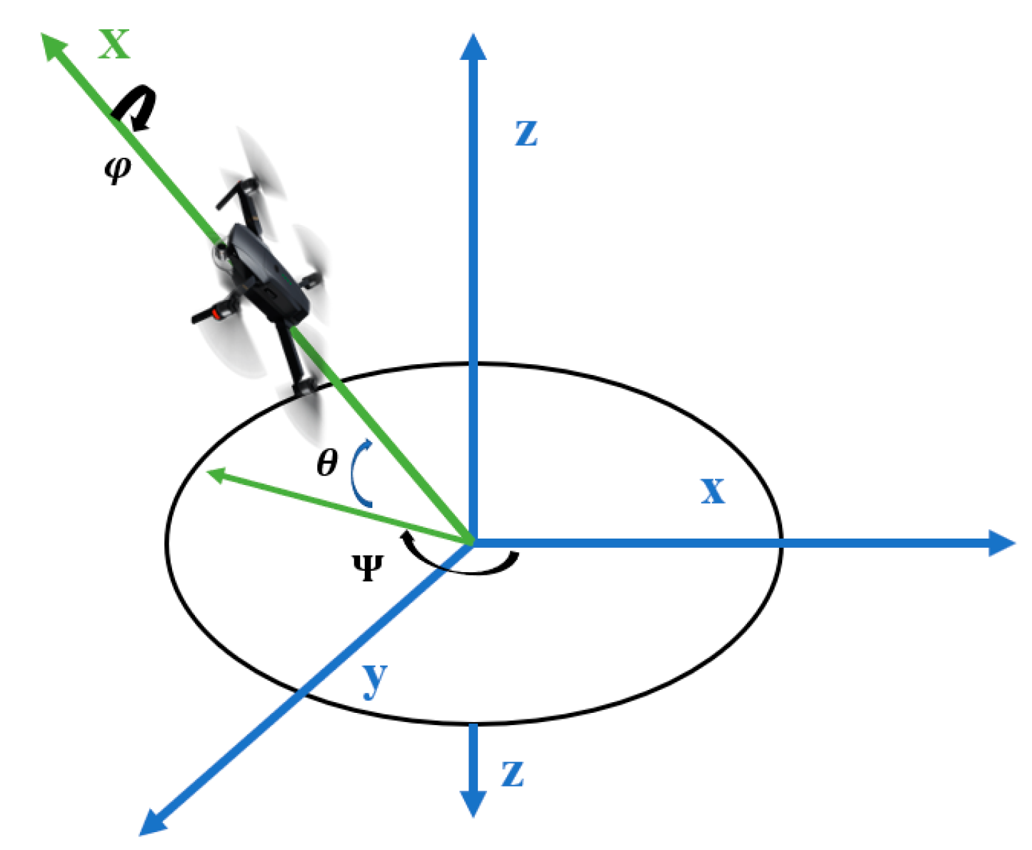
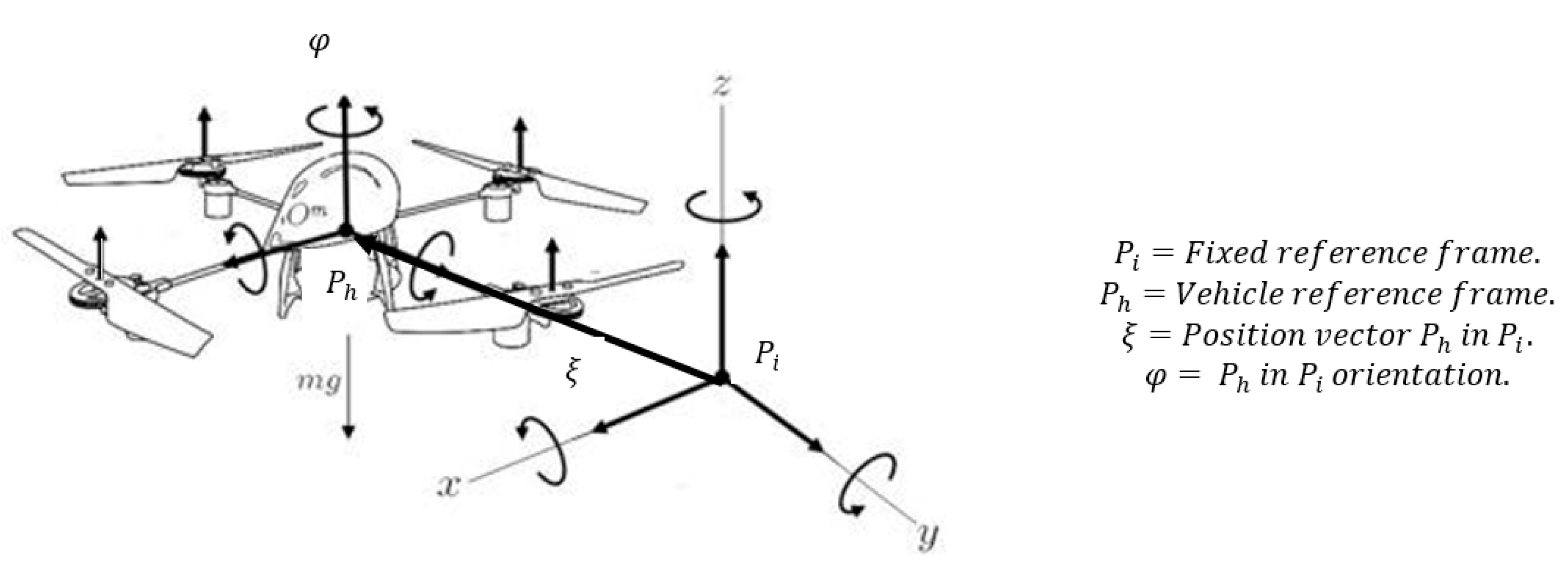
2.1. Mathematical Model of A Six-Degrees-of-Freedom Air Vehicle
2.2. Backstepping Control
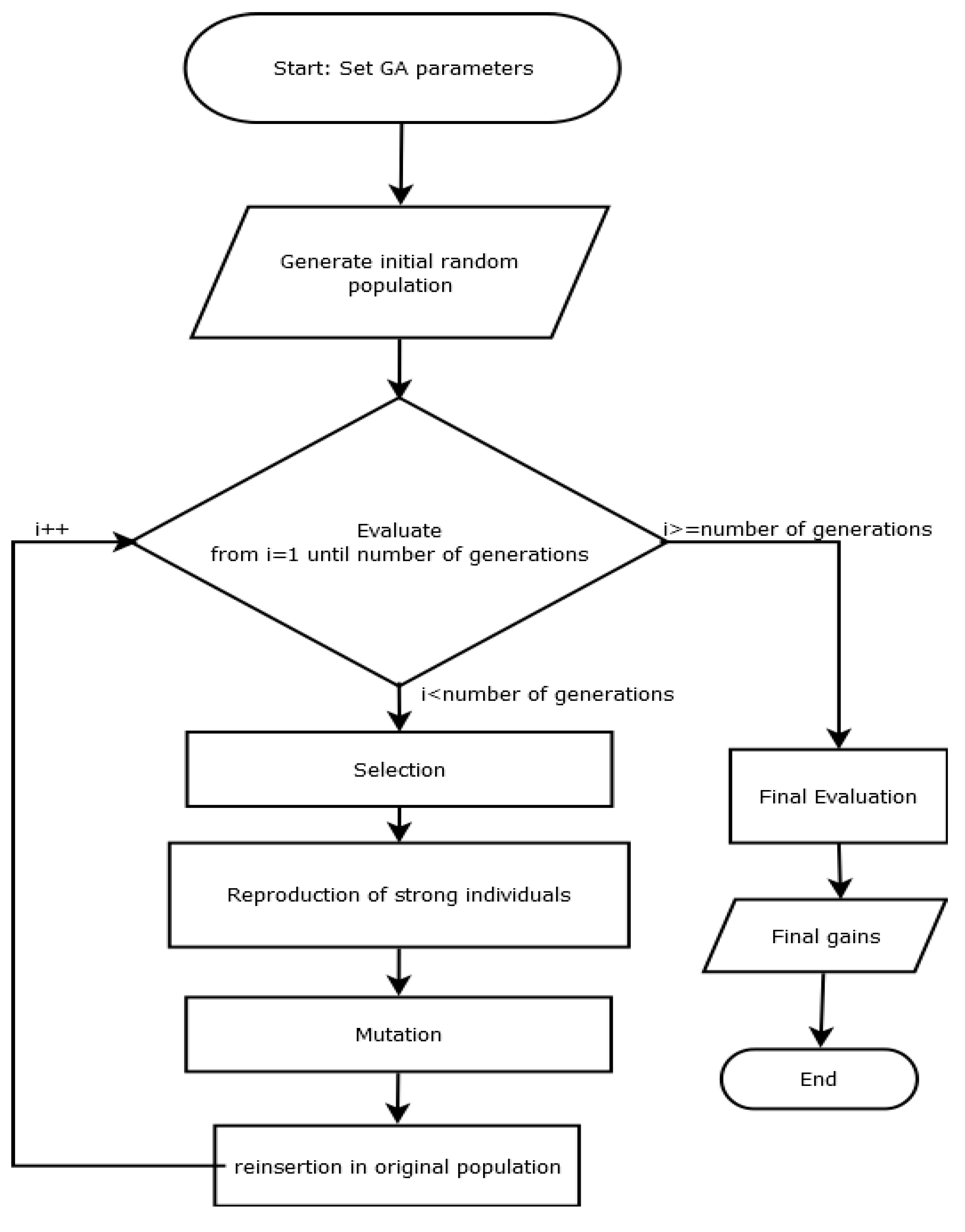
2.3. Tuning the Backstepping Controller Using Genetic Algorithms
3. Results
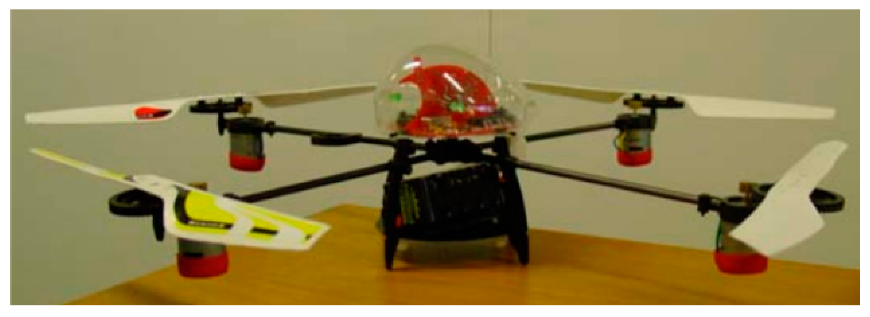
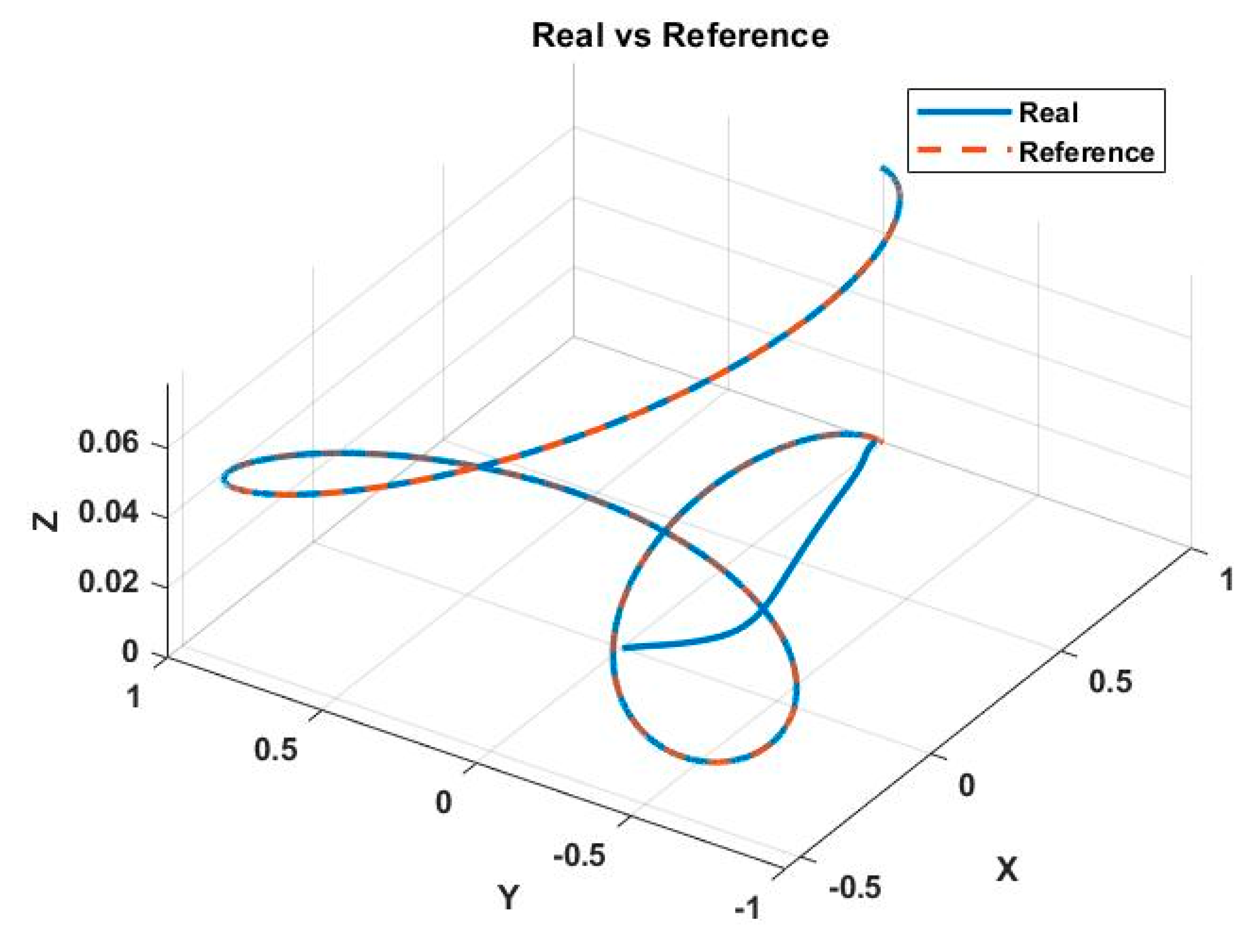
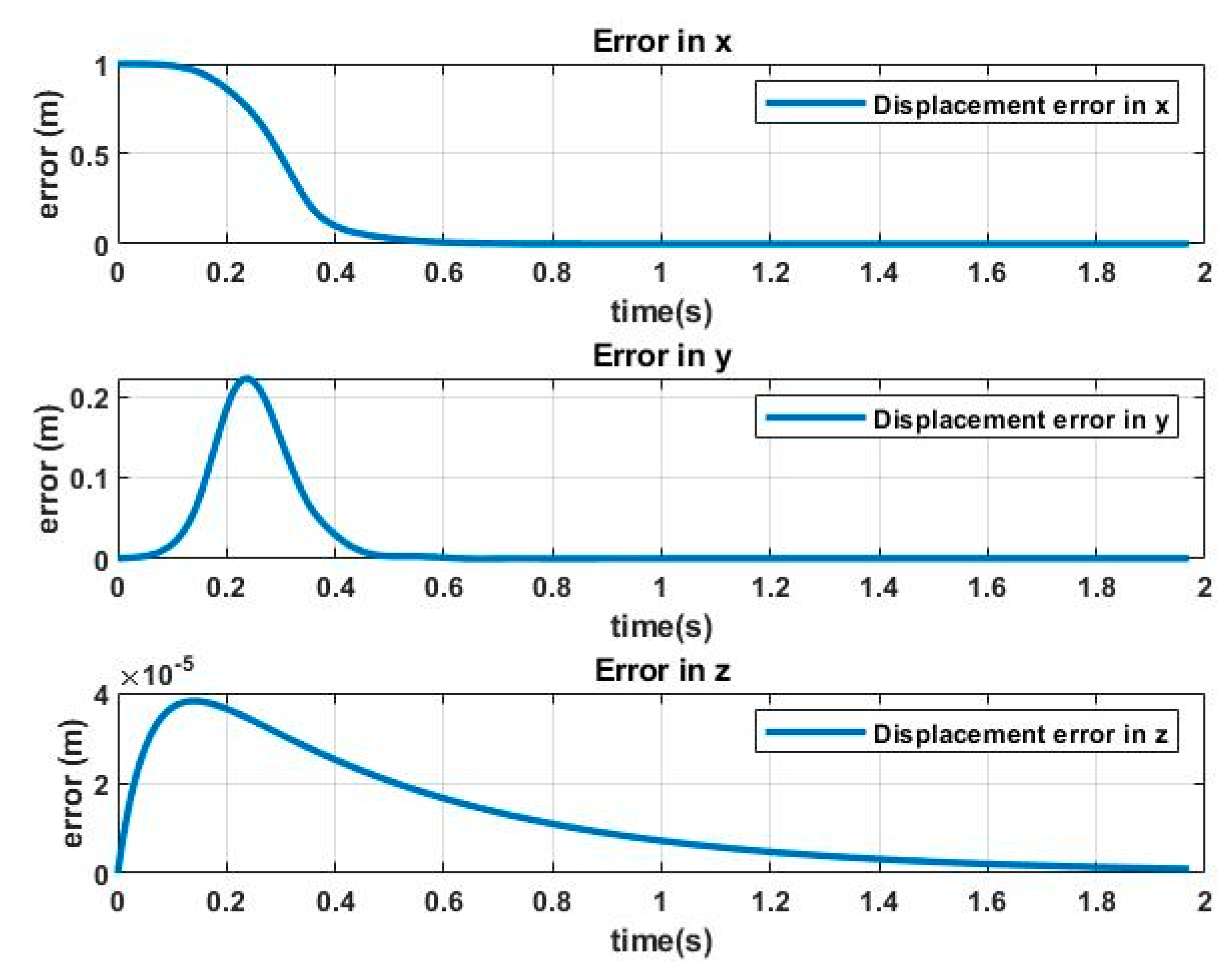
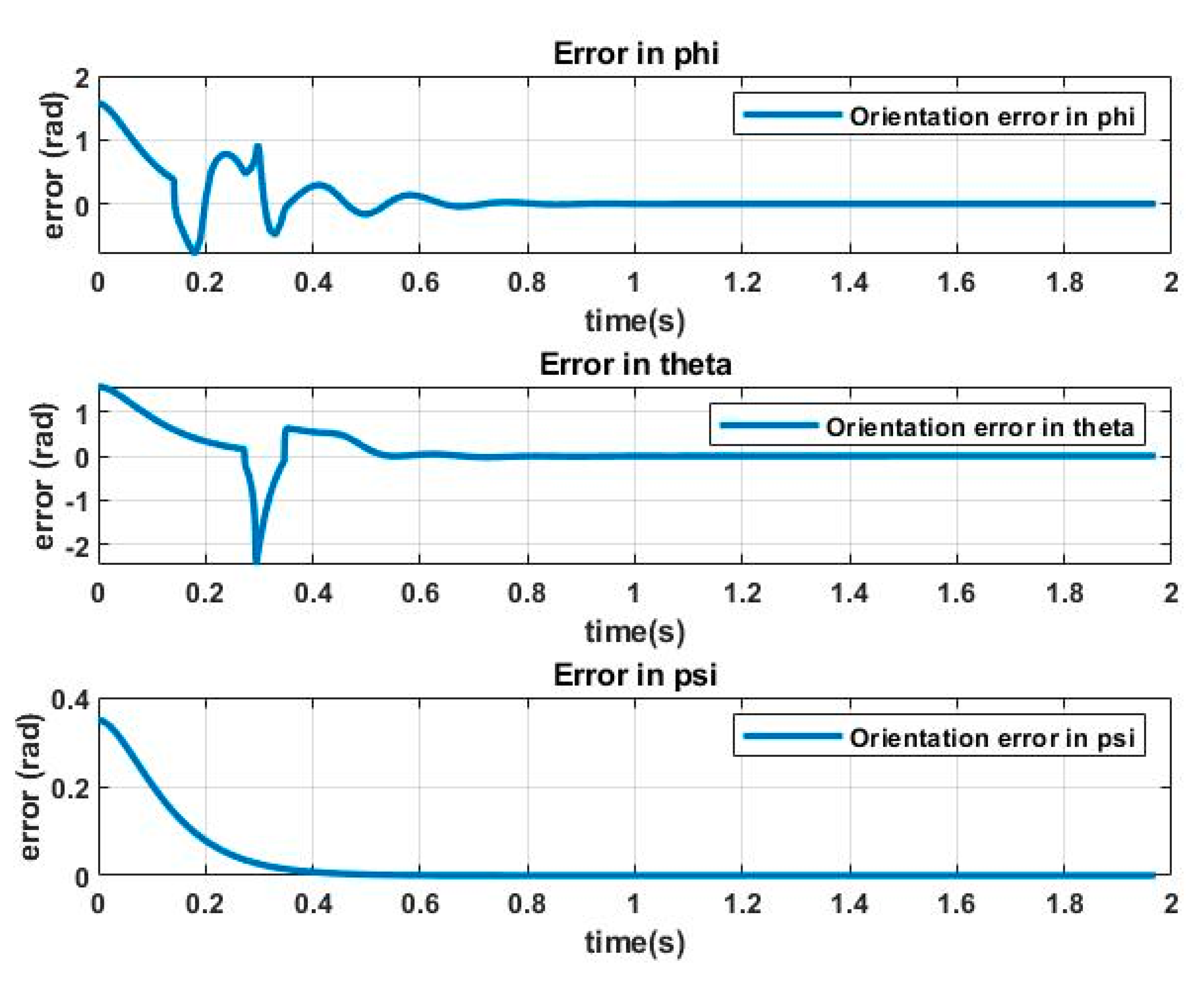
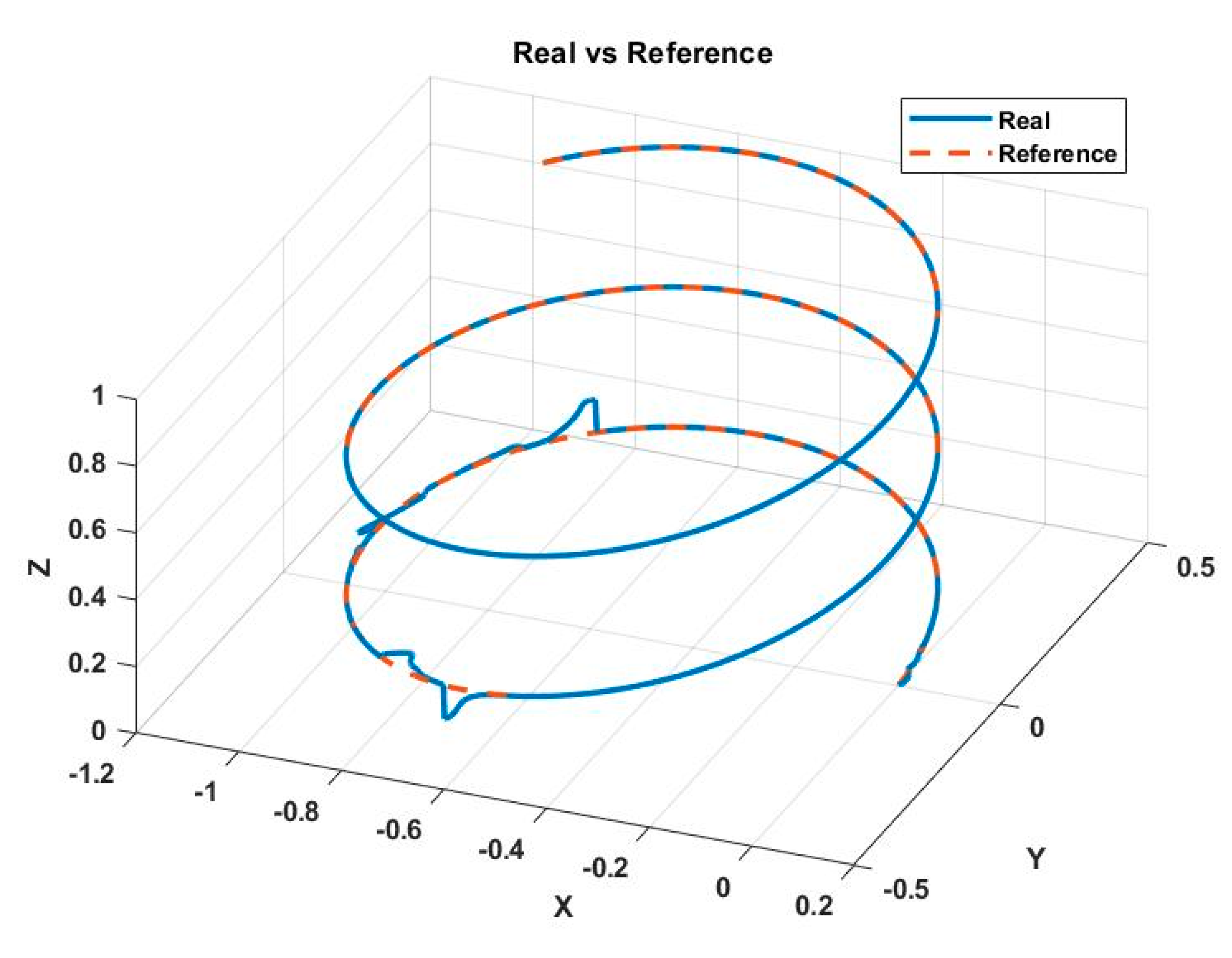
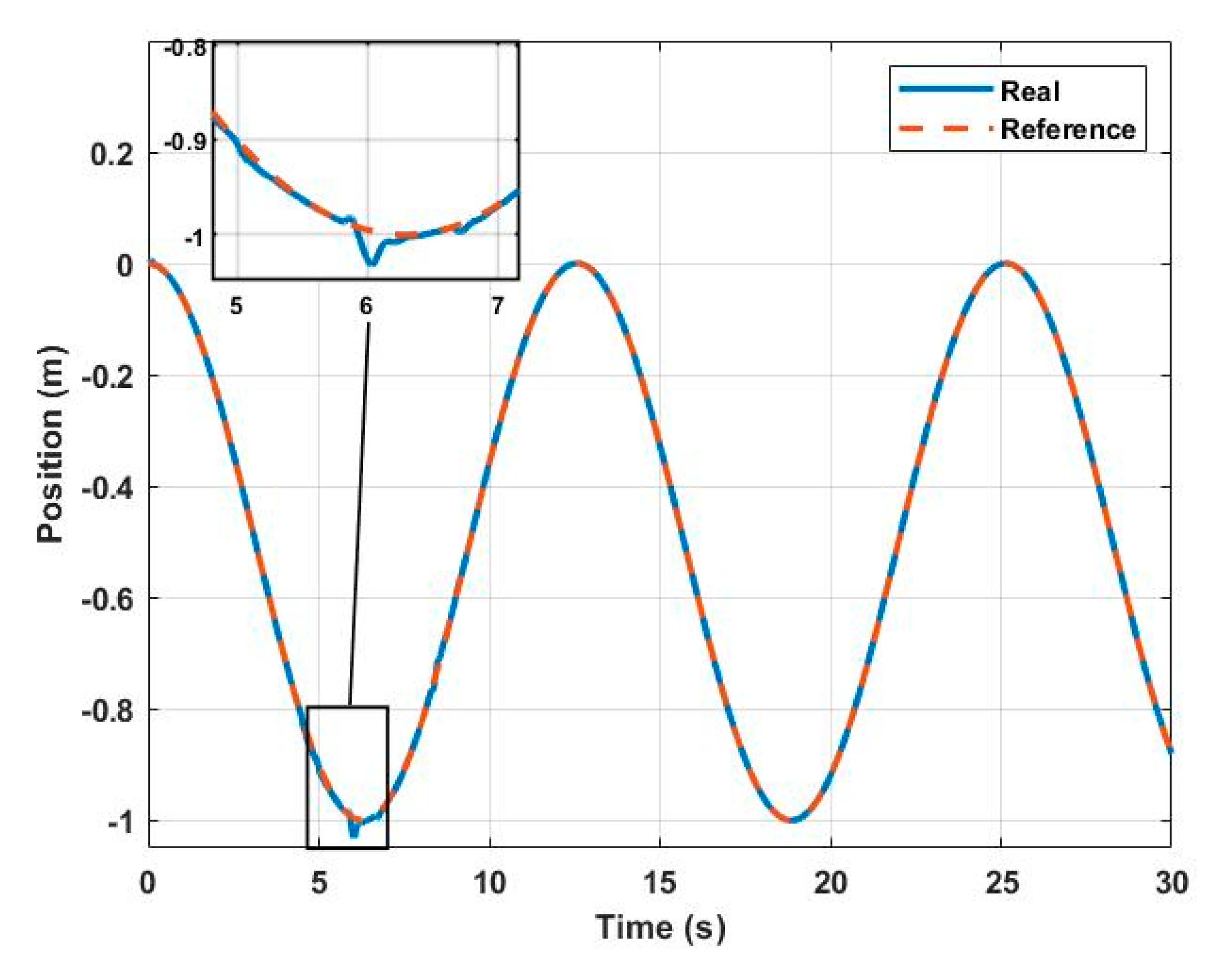
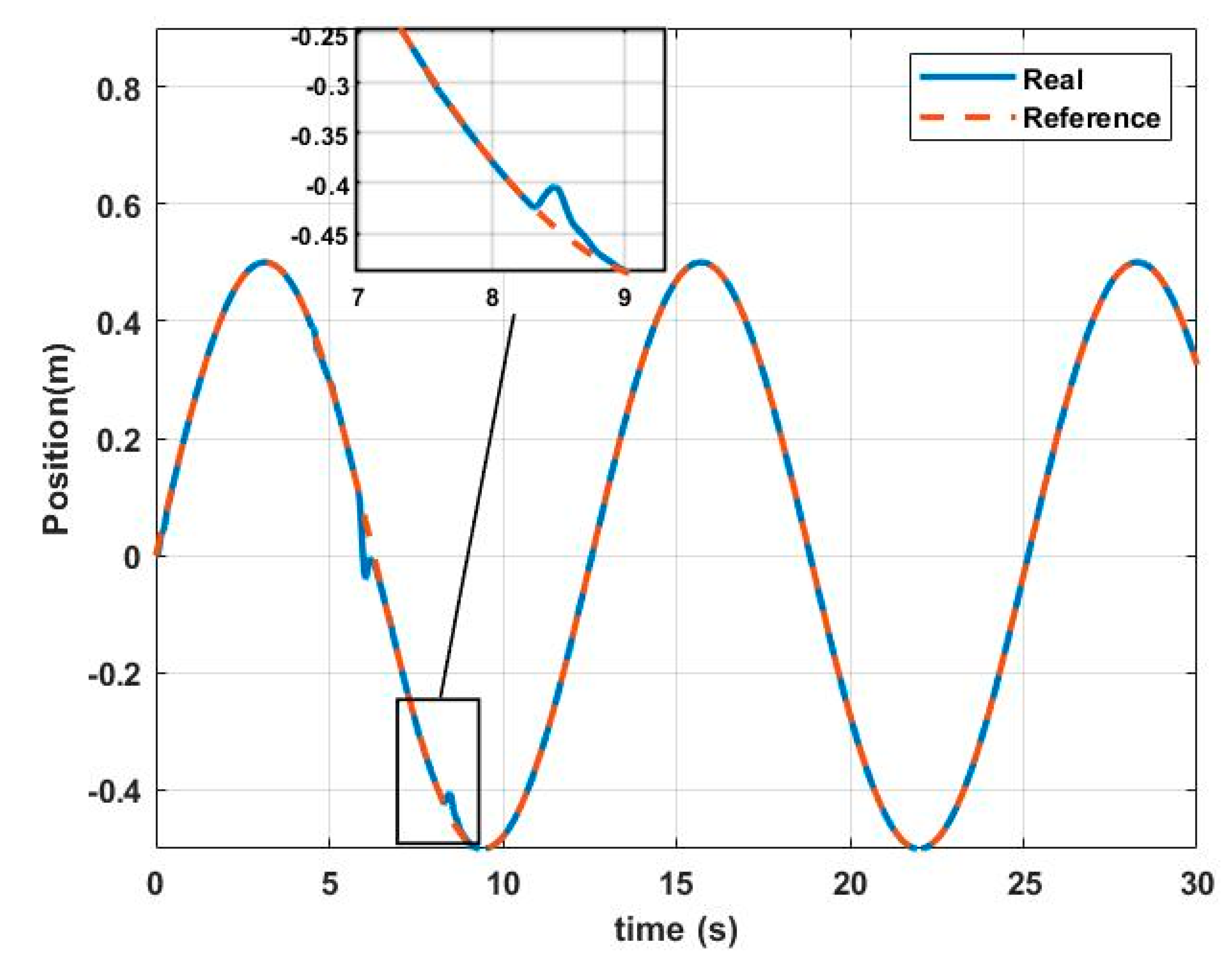
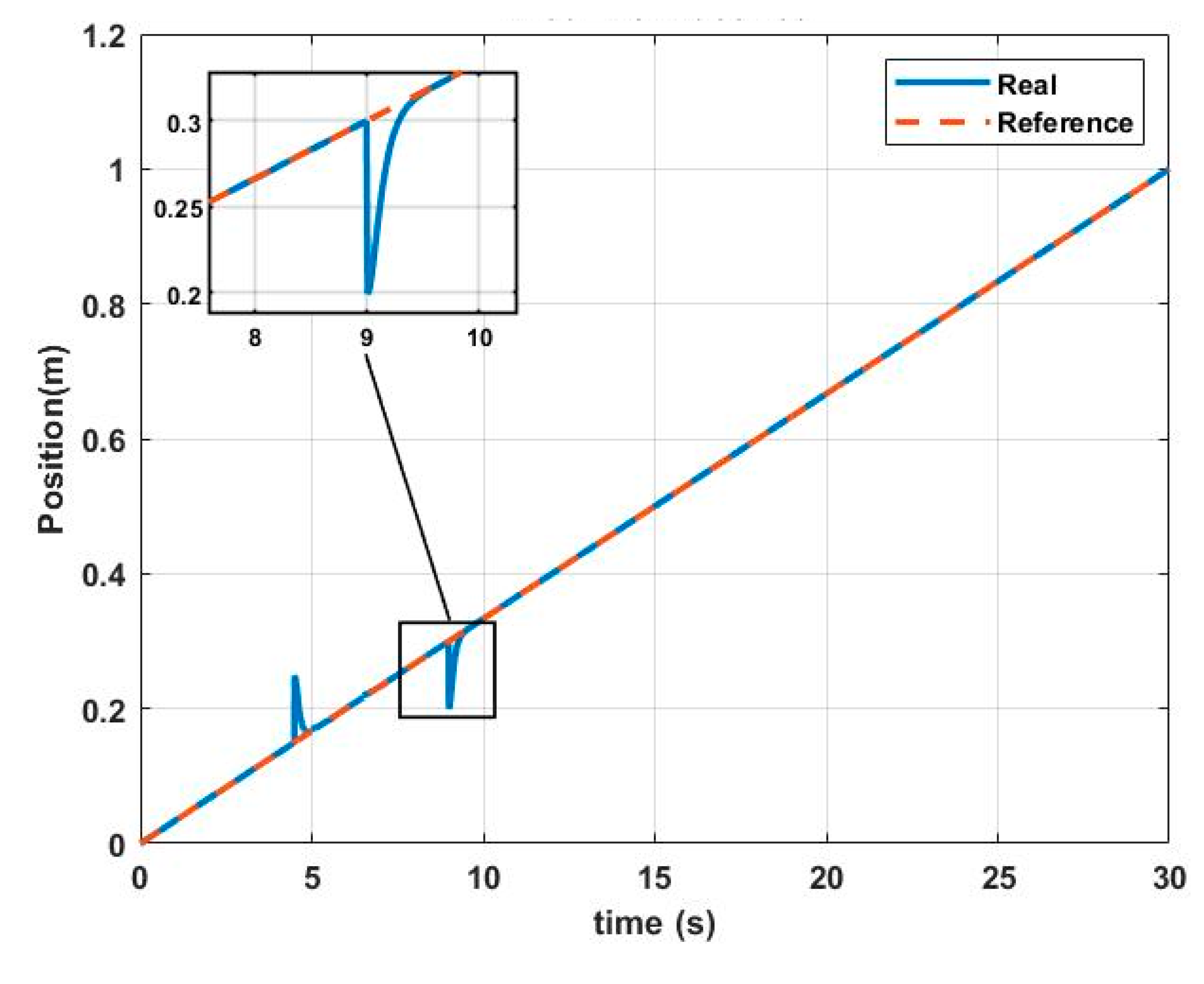
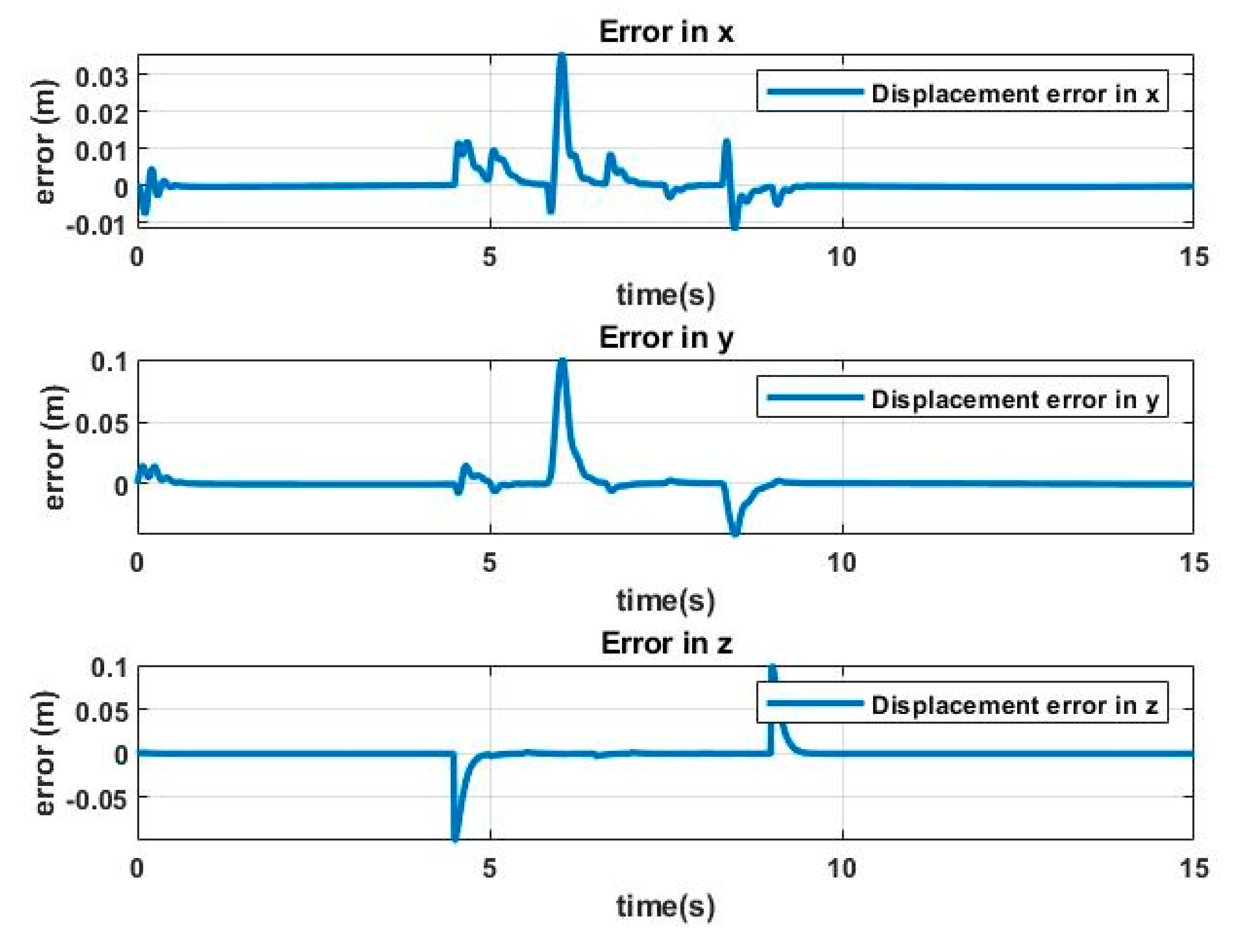
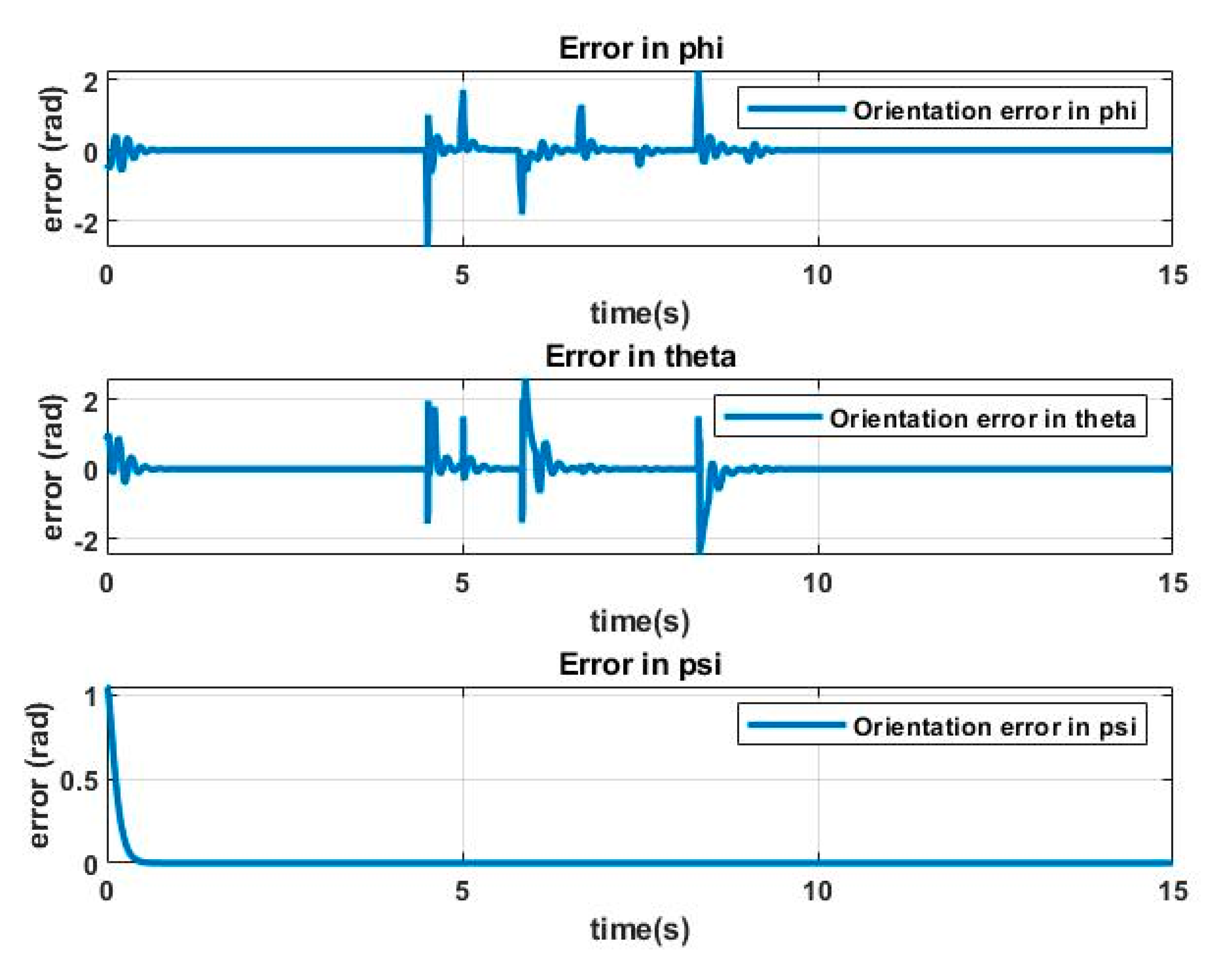
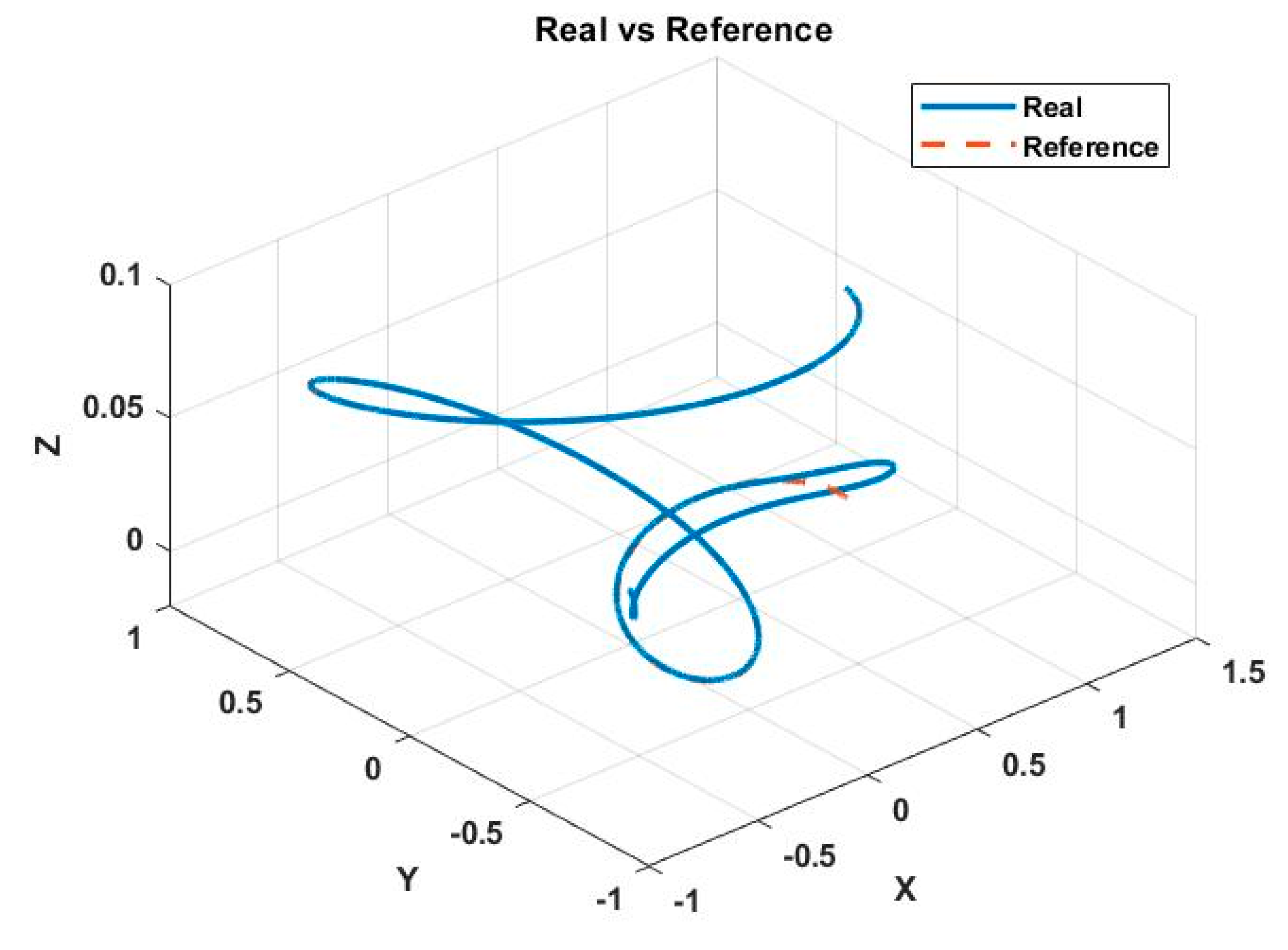
3.1. Experimental Validation
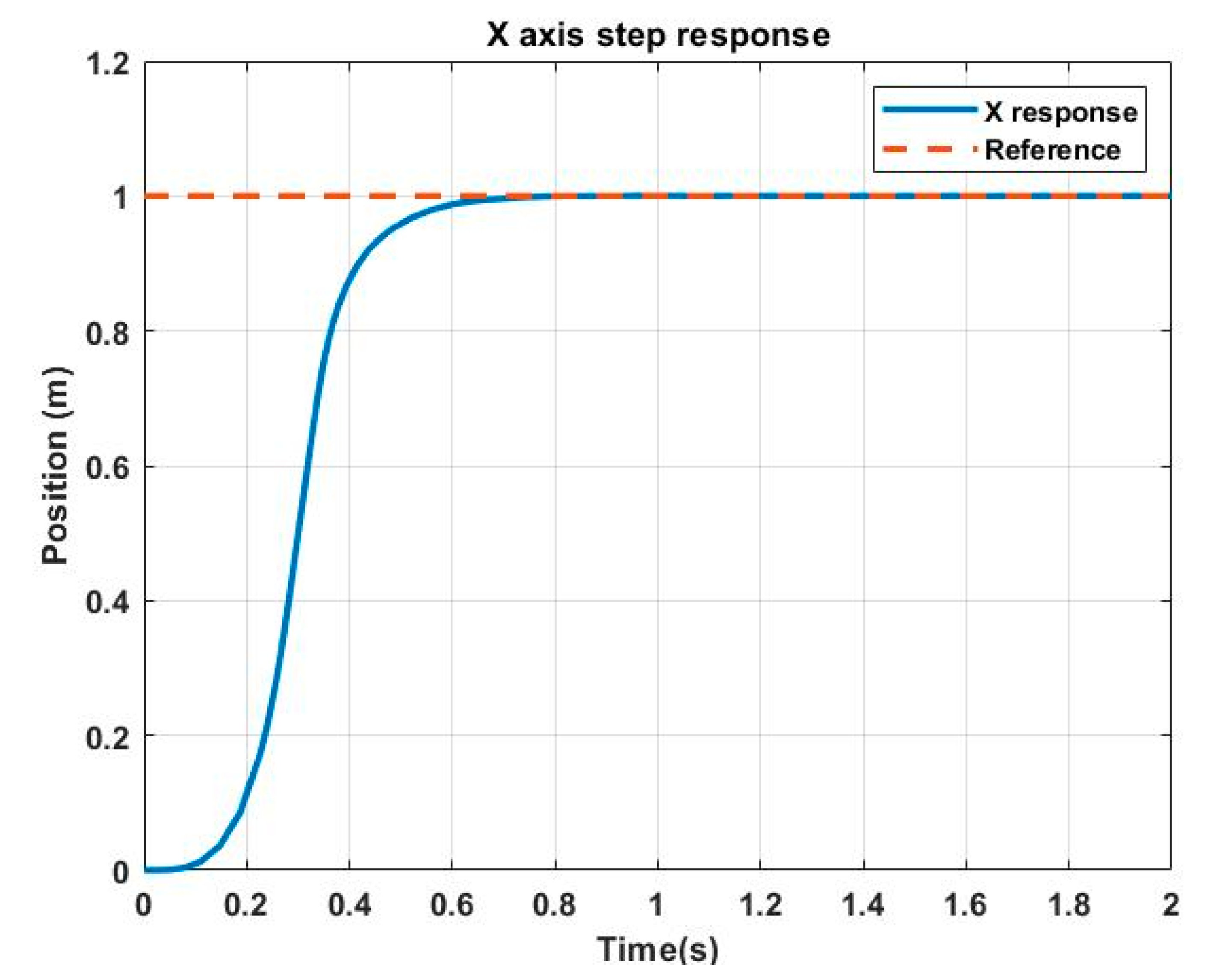
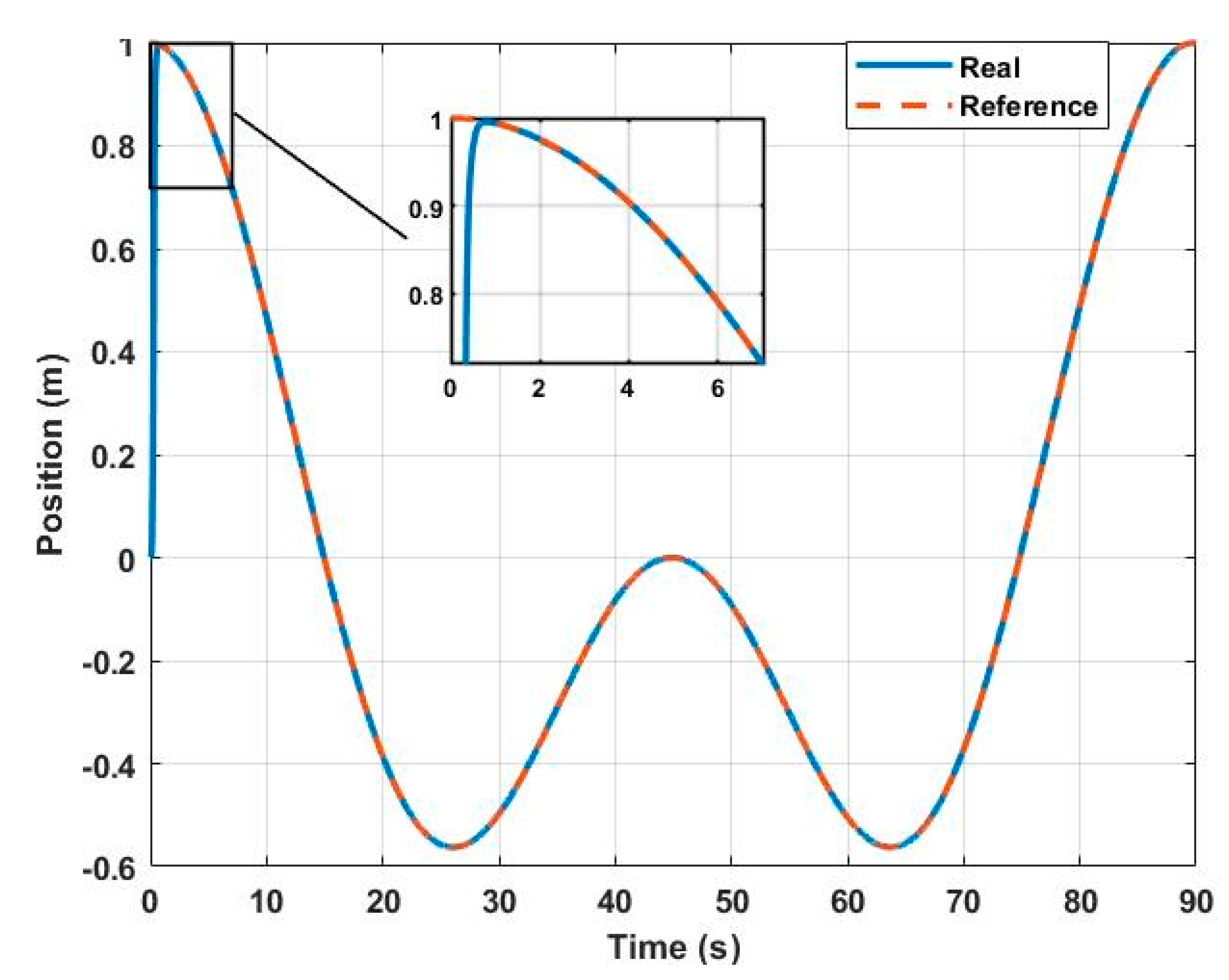
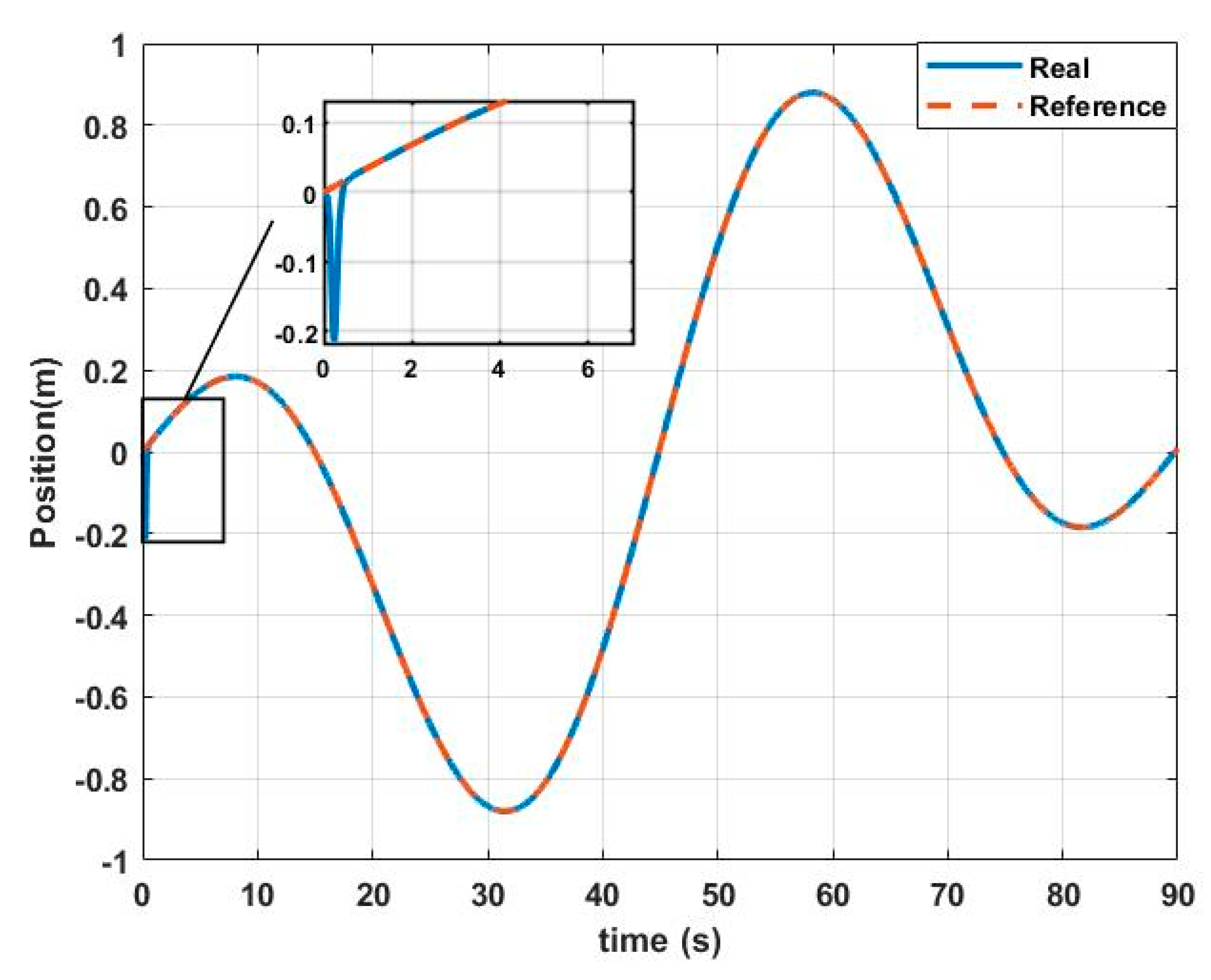
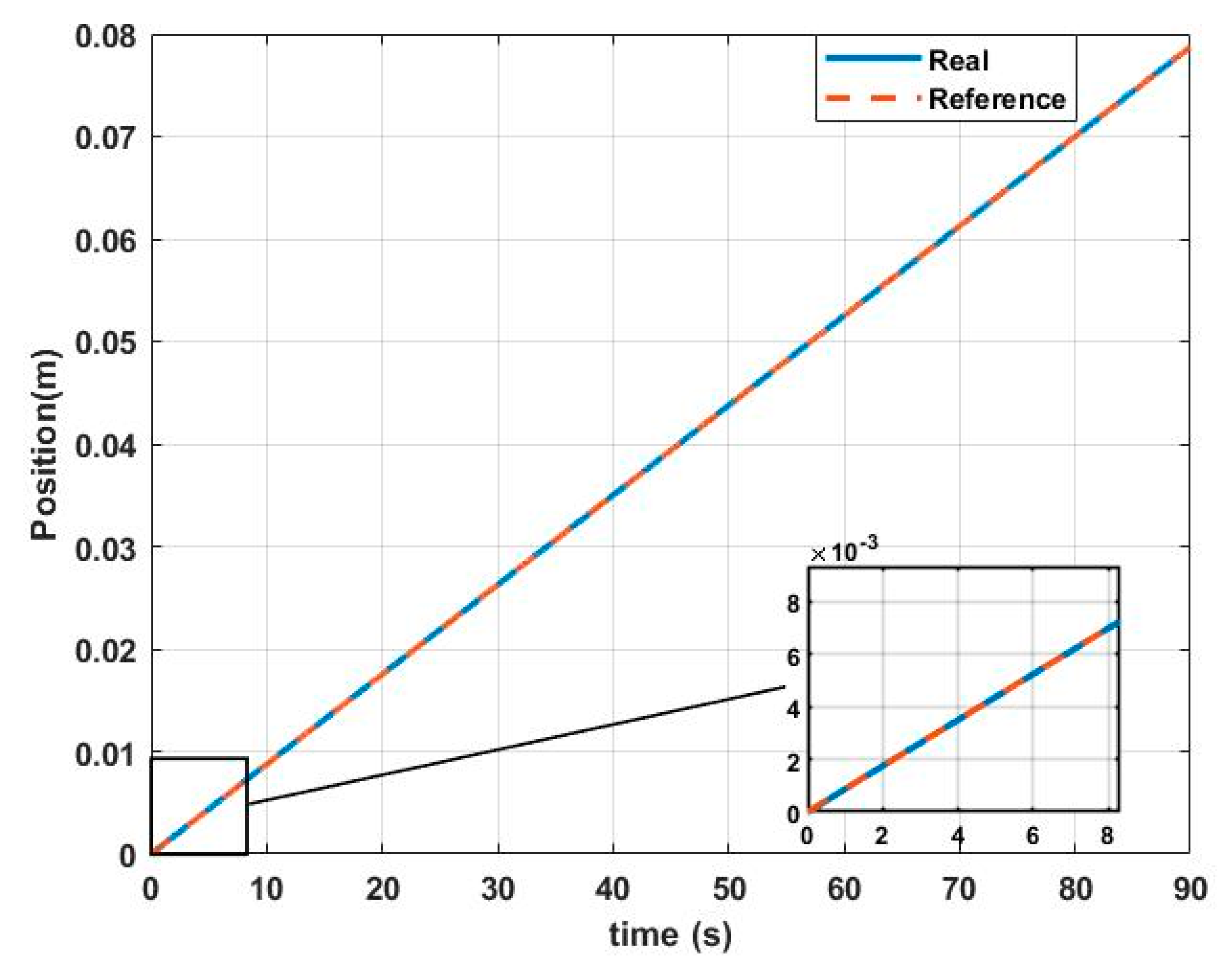
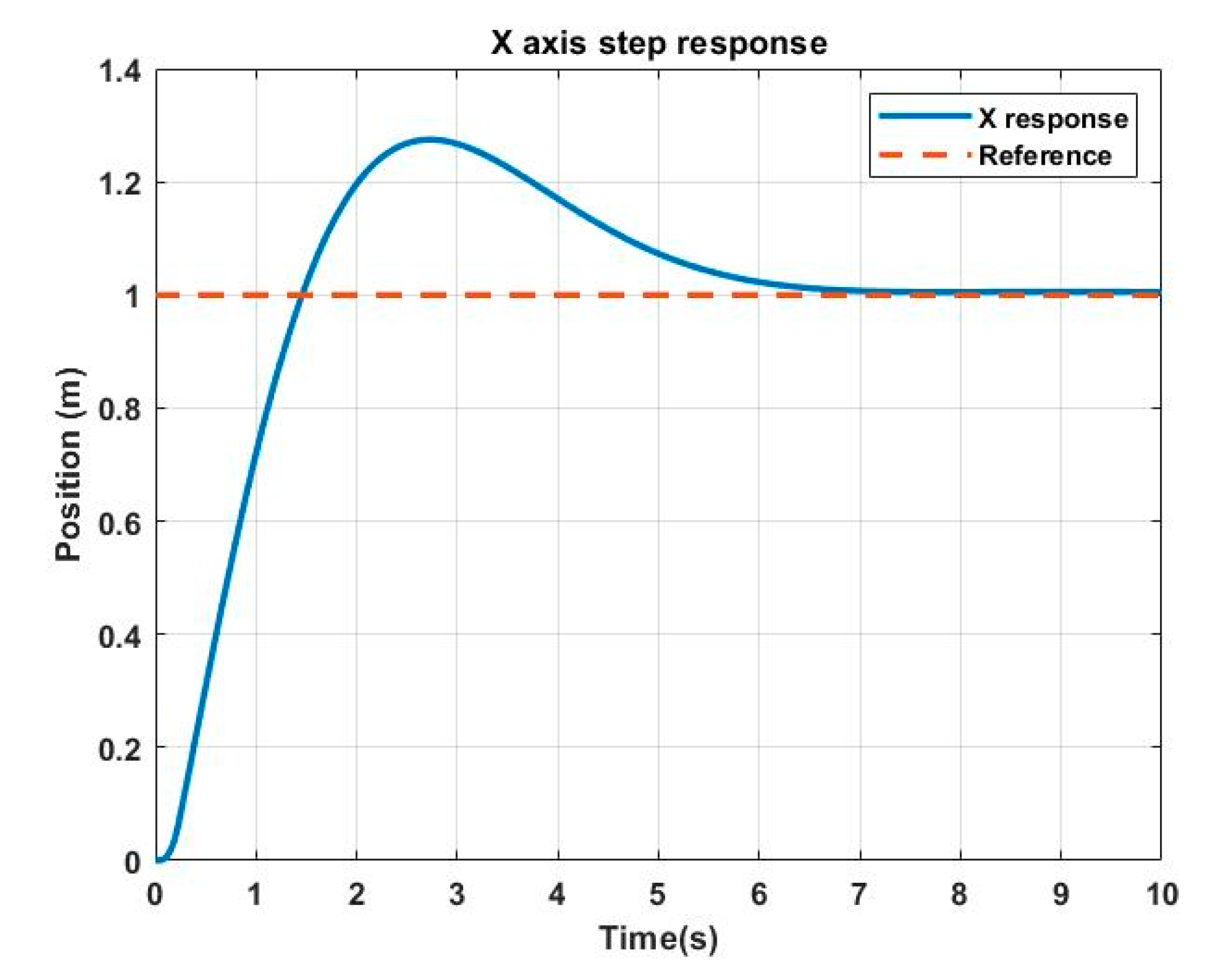
- To prove axis
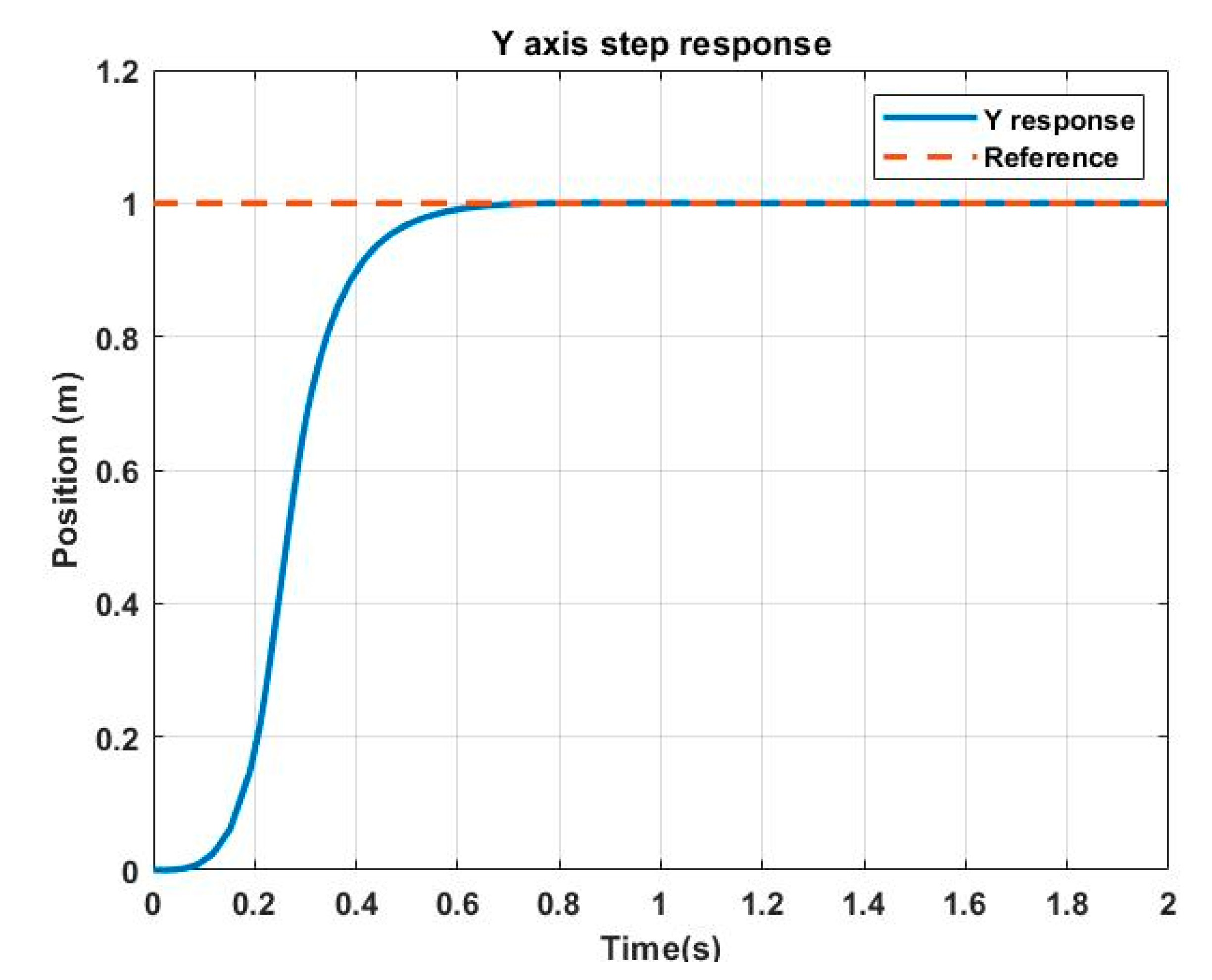
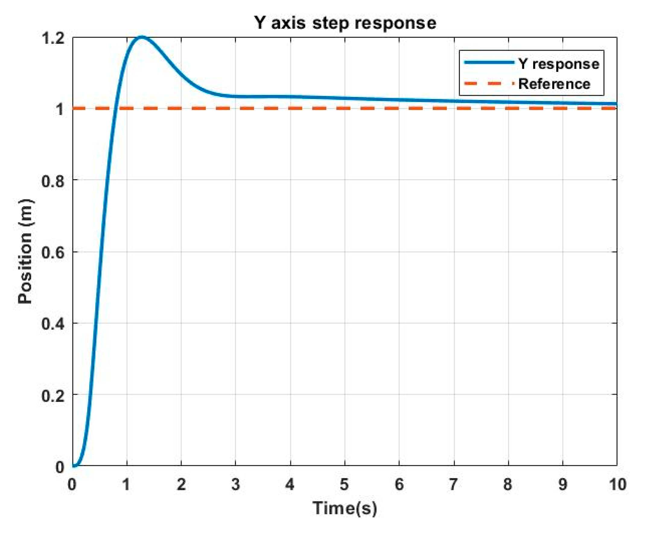
- To prove axis
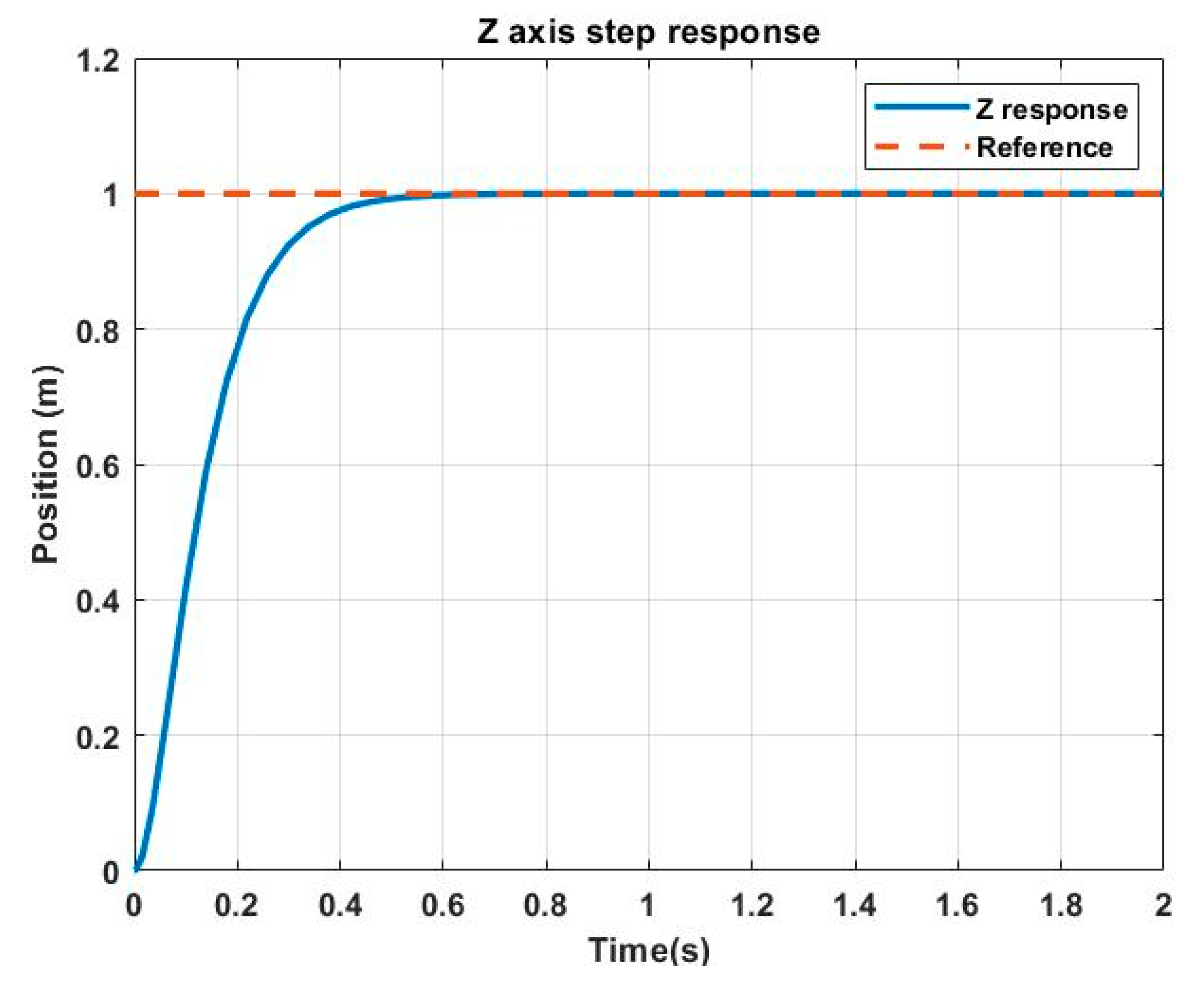
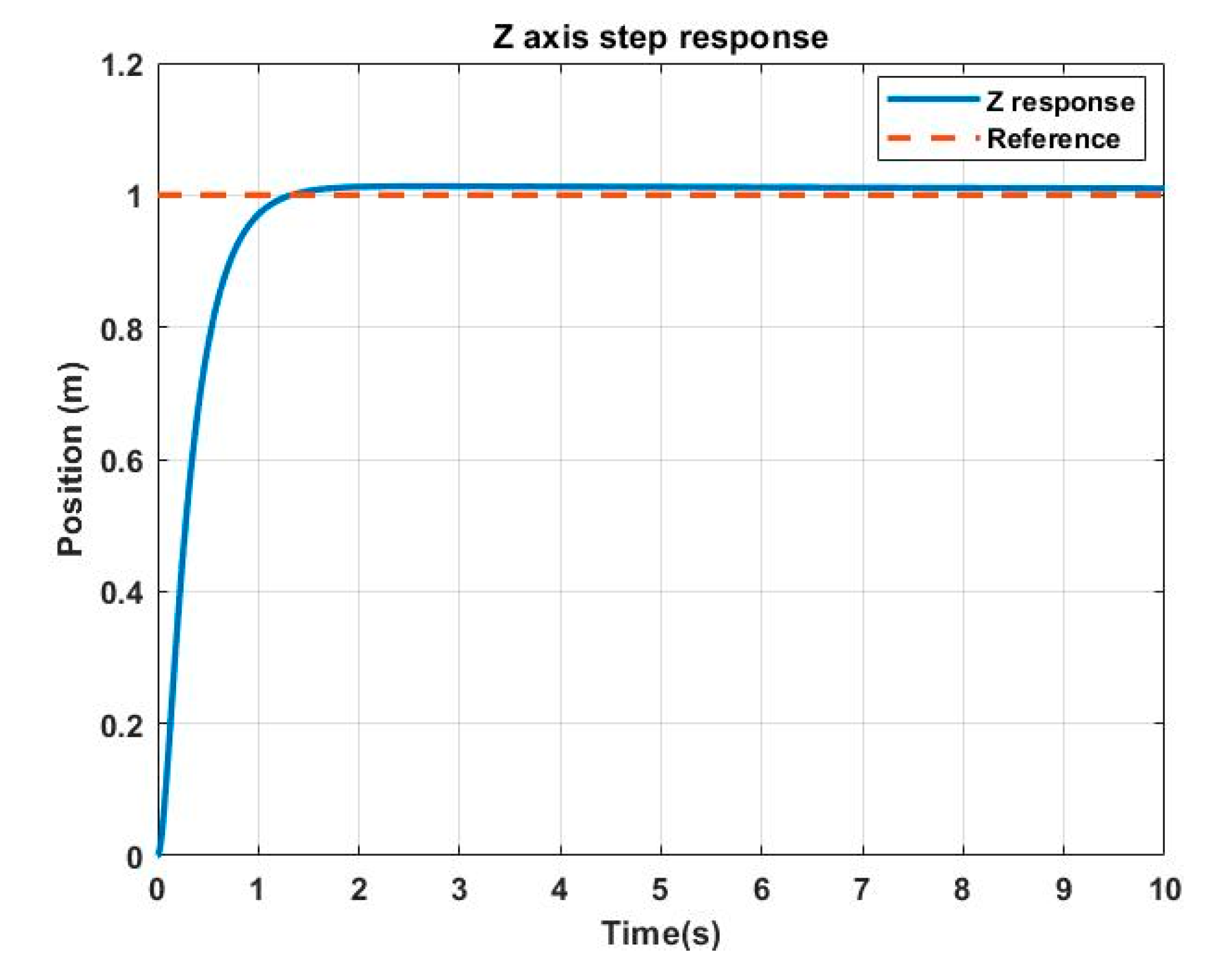
- To prove axis
3.2. PID Controller
4. Conclusions
Author Contributions
Funding
Conflicts of Interest
References
- Xin, J.; Zhong, J.; Yang, F.; Cui, Y.; Sheng, J. An Improved Genetic Algorithm for Path-Planning of Unmanned Surface Vehicle. Sensors 2019, 19, 2640. [Google Scholar] [CrossRef] [PubMed]
- Giernacki, W.; Horla, D.; Baca, T.; Saska, M. Real-Time Model-Free Minimum-Seeking Autotuning Method for Unmanned Aerial Vehicle Controllers Based on Fibonacci-Search Algorithm. Sensors 2019, 19, 312. [Google Scholar] [CrossRef] [PubMed]
- Castano, F.; Beruvides, G.; Villalonga, A.; Haber, R.E. Self-Tuning Method for Increased Obstacle Detection Reliability Based on Internet of Things LiDAR Sensor Models. Sensors 2018, 18, 1508. [Google Scholar] [CrossRef] [PubMed]
- Zemmour, E.; Kurtser, P.; Edan, Y. Automatic Parameter Tuning for Adaptive Thresholding in Fruit Detection. Sensors 2019, 19, 2130. [Google Scholar] [CrossRef]
- Espinoza, K.; Valera-Martínez, D.L.; Torres, J.A.; López-Martínez, A.; Molina-Aiz, F. An Auto-Tuning PI Control System for an Open-Circuit Low-Speed Wind Tunnel Designed for Greenhouse Technology. Sensors 2015, 15, 19723–19749. [Google Scholar] [CrossRef]
- Tang, J.; Zheng, J.; Wang, Y.; Yu, L.; Zhan, E.; Song, Q. Self-Tuning Threshold Method for Real-Time Gait Phase Detection Based on Ground Contact Forces Using FSRs. Sensors 2018, 18, 481. [Google Scholar] [CrossRef]
- Lee, C.; Chen, R. Optimal Self-Tuning PID Controller Based on Low Power Consumption for a Server Fan Cooling System. Sensors 2015, 15, 11685–11700. [Google Scholar] [CrossRef]
- Besada, J.A.; Bergesio, L.; Campaña, I.; Vaquero-Melchor, D.; Lopez-Araquistain, J.; Bernardos, A.M.; Casar, J.R. Drone Mission Definition and Implementation for Automated Infrastructure Inspection Using Airborne Sensors. Sensors 2018, 18, 1170. [Google Scholar] [CrossRef]
- Hamza, M.; Jehangir, A.; Ahmad, T.; Sohail, A.; Naeem, M. Design of surveillance drone with X-ray camera, IR camera and metal detector. In Proceedings of the 2017 Ninth International Conference on Ubiquitous and Future Networks (ICUFN), Milan, Italy, 4–7 July 2017; pp. 111–114. [Google Scholar]
- Pedro, J.O.; Dangor, M.; Kala, P.J. Differential evolution-based PID control of a quadrotor system for hovering application. In Proceedings of the 2016 IEEE Congress on Evolutionary Computation (CEC), Vancouver, BC, Canada, 24–29 July 2016; pp. 2791–2798. [Google Scholar]
- Zheng, H.; Zeng, Q.; Chen, W.; Zhu, H.; Chen, C. Improved PID control algorithm for quadrotor based on MCS. In Proceedings of the 2016 IEEE Chinese Guidance, Navigation and Control Conference (CGNCC), Nanjing, China, 12–14 August 2016; pp. 1780–1783. [Google Scholar]
- Mo, H.; Farid, G. Nonlinear and Adaptive Intelligent Control Techniques for Quadrotor UAV—A Survey. Asian J. Control. 2019, 21, 989–1008. [Google Scholar] [CrossRef]
- Pervaiz, M.; Khan, Q.; Bhatti, A.I.; Malik, S.A. Dynamical Adaptive Integral Sliding Backstepping Control of Nonlinear Nontriangular Uncertain Systems. Math. Probl. Eng. 2014, 2014, 1–14. [Google Scholar] [CrossRef]
- Knöös, J.; Robinson, J.W.C.; Berefelt, F. Nonlinear Dynamic Inversion and Block Backstepping: A Comparison. In Proceedings of the AIAA Guidance, Navigation, and Control Conference 2012, Minneapolis, MN, USA, 13–16 August 2012. [Google Scholar] [CrossRef]
- Koshkouei, A.; Zinober, A. Adaptive Sliding Backstepping Control of Nonlinear Semi-Strict Feedback form Systems. In Proceedings of the 7th IEEE Mediterranean Control Conference, Haifa, Israel, 28–30 June 1999. [Google Scholar]
- Koshkouei, A.; Burnham, K.J. Adaptive backstepping sliding mode control for feedforward uncertain systems. Int. J. Syst. Sci. 2011, 42, 1935–1946. [Google Scholar] [CrossRef]
- Koshkouei, A.J.; Mills, R.E.; Zinober, A.S.I. Adaptive Backstepping Control. In Variable Structure Systems: Towards the 21st Century; Yu, X., Xu, J.-X., Eds.; Lecture Notes in Control and Information Sciences; Springer: Berlin/Heidelberg, Germany, 2002; Volume 274, pp. 129–153. ISBN 978-3-540-45666-7. [Google Scholar]
- Gao, Y.; Tian, D.; Wang, Y. Fuzzy Self-tuning Tracking Differentiator for Motion Measurement Sensors and Application in Wide-Bandwidth High-accuracy Servo Control. Sensors 2020, 20, 948. [Google Scholar] [CrossRef] [PubMed]
- Lee, T.; Leok, M.; McClamroch, N.H.; Leoky, M. Geometric tracking control of a quadrotor UAV on SE (3). In Proceedings of the 49th IEEE Conference on Decision and Control (CDC 2010), Atlanta, GA, USA, 15–17 December 2010; pp. 5420–5425. [Google Scholar]
- Das, A.; Lewis, F.; Subbarao, K. Sliding Mode Approach to Control Quadrotor Using Dynamic Inversion. Chall. Paradig. Appl. Robust Control 2011, 3–24. [Google Scholar] [CrossRef]
- Sieberling, S.; Chu, Q.; Mulder, J.A. Robust Flight Control Using Incremental Nonlinear Dynamic Inversion and Angular Acceleration Prediction. J. Guid. Control. Dyn. 2010, 33, 1732–1742. [Google Scholar] [CrossRef]
- Ansari, U.; Bajodah, A.H. Robust generalized dynamic inversion based control of autonomous underwater vehicles. SAGE J. 2017. [Google Scholar] [CrossRef]
- Muliadi, J.; Kusumoputro, B. Neural Network Control System of UAV Altitude Dynamics and Its Comparison with the PID Control System. J. Adv. Transp. 2018, 2018, 1–18. [Google Scholar] [CrossRef]
- Kusumoputro, B.; Priandana, K.; Wahab, W. System identification and control of pressure process rig® system using backpropagation neural networks. ARPN J. Eng. Appl. Sci. 2015, 10, 7190–7195. [Google Scholar]
- Hernández-Alvarado, R.; García-Valdovinos, L.G.; Salgado-Jiménez, T.; Gómez-Espinosa, A.; Fonseca-Navarro, F. Neural Network-Based Self-Tuning PID Control for Underwater Vehicles. Sensors 2016, 16, 1429. [Google Scholar] [CrossRef] [PubMed]
- Reyad, M.; Arafa, M.; Sallam, E.A. An optimal PID controller for a qaudrotor system based on DE algorithm. In Proceedings of the 11th IEEE International Conference on Computer Engineering and Systems (ICCES), Cairo, Egypt, 20–21 December 2016; pp. 444–451. [Google Scholar]
- Mellinger, D.; Kumar, V. Minimum snap trajectory generation and control for quadrotors. In Proceedings of the 2011 IEEE International Conference on Robotics and Automation, Shanghai, China, 9–13 May 2011; pp. 2520–2525. [Google Scholar]
- Tesch, D.A.; Eckhard, D.; Guarienti, W.C. Pitch and Roll control of a Quadcopter using Cascade Iterative Feedback Tuning. In Proceedings of the 4th IFAC Symposium on Telematics Applications TA 2016, Porto Alwegre, Brasil, 6–9 November 2016. [Google Scholar]
- Jokar, A.; Godarzi, A.A.; Saber, M.; Shafii, M.B. Simulation and optimization of a pulsating heat pipe using artificial neural network and genetic algorithm. Heat Mass Transf. 2016, 52, 2437–2445. [Google Scholar] [CrossRef]
- Li, Y.; Song, S. A survey of control algorithms for Quadrotor Unmanned Helicopter. In Proceedings of the Fifth International Conference on Advanced Computational Intelligence (ICACI 2012), Nanjing, China, 18–20 October 2012; pp. 365–369. [Google Scholar]
- Yu, G.; Doukhi, O.; Fayjie, A.R.; Lee, D.J. Intelligent Controller Design for Quad-Rotor Stabilization in Presence of Parameter Variations. J. Adv. Transp. 2017, 2017. [Google Scholar] [CrossRef]
- Sadeghzadeh, I.; Abdolhosseini, M.; Zhang, Y. Payload Drop Application of Unmanned Quadrotor Helicopter Using Gain-Scheduled PID and Model Predictive Control Techniques. Lect. Notes Comput. Sci. 2012, 7506, 386–395. [Google Scholar]
- D’Amato, E.; Di Francesco, G.; Notaro, I.; Tartaglione, G.; Mattei, M. Nonlinear Dynamic Inversion and Neural Networks for a Tilt Tri-Rotor UAV. IFAC-PapersOnLine 2015, 48, 162–167. [Google Scholar] [CrossRef]
- Davoudi, B.; Taheri, E.; Duraisamy, K.; Jayaraman, B.; Kolmanovsky, I. Quad-Rotor Flight Simulation in Realistic Atmospheric Conditions. AIAA J. 2020, 58, 1992–2004. [Google Scholar] [CrossRef]
- Lee, J. Optimization of a modular drone delivery system. In Proceedings of the 2017 Annual IEEE International Systems Conference (SysCon), Montreal, QC, Canada, 24–27 April 2017; pp. 1–8. [Google Scholar]
- Berning, A.W.; Taheri, E.; Girard, A.; Kolmanovsky, I. Rapid Uncertainty Propagation and Chance-Constrained Trajectory Optimization for Small Unmanned Aerial Vehicles. In Proceedings of the 2018 Annual American Control Conference (ACC), Milwaukee, WI, USA, 27–29 June 2018; pp. 3183–3188. [Google Scholar]
- Ventura Diaz, P.; Yoon, S. High-Fidelity Computational Aerodynamics of Multi-Rotor Unmanned Aerial Vehicles. In Proceedings of the 2018 AIAA SciTech Forum, American Institute of Aeronautics and Astronautics, Kissimmee, FL, USA, 8–12 January 2018. [Google Scholar]
- Mishra, A.; Davoudi, B.; Duraisamy, K. Multiple-Fidelity Modeling of Interactional Aerodynamics. J. Aircr. 2018, 55, 1839–1854. [Google Scholar] [CrossRef]
- Lim, S.P.; Haron, H. Performance comparison of Genetic Algorithm, Differential Evolution and Particle Swarm Optimization towards benchmark functions. In Proceedings of the 2013 IEEE Conference on Open Systems (ICOS 2013), Kuching, Malaysia, 2–4 December 2013; pp. 41–46. [Google Scholar]
- Winiczenko, R.; Górnicki, K.; Kaleta, A.; Janaszek-Mańkowska, M. Optimisation of ANN topology for predicting the rehydrated apple cubes colour change using RSM and GA. Neural Comput. Appl. 2018, 30, 1795–1809. [Google Scholar] [CrossRef] [PubMed]
- McKerrow, P. Modelling the Draganflyer four-rotor helicopter. In Proceedings of the 2004 IEEE International Conference on Robotics and Automation, New Orleans, LA, USA, 26 April–1 May 2004; Volume 4, pp. 3596–3601. [Google Scholar] [CrossRef]
- Yim, S. Comparison among Active Front, Front Independent, 4-Wheel and 4-Wheel Independent Steering Systems for Vehicle Stability Control. Electronics 2020, 9, 798. [Google Scholar] [CrossRef]
- Kong, W.; Zhou, D.; Yang, Z.; Zhao, Y.; Zhang, K. UAV Autonomous Aerial Combat Maneuver Strategy Generation with Observation Error Based on State-Adversarial Deep Deterministic Policy Gradient and Inverse Reinforcement Learning. Electronics 2020, 9, 1121. [Google Scholar] [CrossRef]
- Zhang, C.; Zhou, L.; Li, Y.; Fan, Y. A Dynamic Path Planning Method for Social Robots in the Home Environment. Electronics 2020, 9, 1173. [Google Scholar] [CrossRef]
- Wei, Y.; Hong, T.; Kadoch, M. Improved Kalman Filter Variants for UAV Tracking with Radar Motion Models. Electronics 2020, 9, 768. [Google Scholar] [CrossRef]
- Trujillo, J.-C.; Munguía, R.; Urzua, S.; Grau, A. Cooperative Visual-SLAM System for UAV-Based Target Tracking in GPS-Denied Environments: A Target-Centric Approach. Electronics 2020, 9, 813. [Google Scholar] [CrossRef]
- Masood, K.; Molfino, R.; Zoppi, M. Simulated Sensor Based Strategies for Obstacle Avoidance Using Velocity Profiling for Autonomous Vehicle FURBOT. Electronics 2020, 9, 883. [Google Scholar] [CrossRef]


| Parameter | Value | Description |
|---|---|---|
| Size of the population | Quantity of initial α pairs. | |
| Generations | Number of iterations in which the algorithm will search. | |
| Range | Maximum value of each α. | |
| Mutation probability | Probability that a selected gene will undergo a mutation. | |
| Biological pressure | Percentage of genes that will reproduce. | |
| Model | Vector that will use a genetic model to follow; is the establishment time and is the maximum over-impulse . | |
| Individual | Vector with four random gains. | |
| Selection method | Rank Selection | The individual with the best fitness gets rank and the worst individual gets rank . The selection probability is |
| Crossover type | Single Point Crossover | A random point is selected for swapping chromosomes. |
| Gain | Result | Gain | Result |
|---|---|---|---|
| Axis | ||
|---|---|---|
| X | ||
| X | Y | Z | Roll | Pitch | Yaw | |
|---|---|---|---|---|---|---|
| Kp | 32 | 28 | 25 | 15 | 15 | 5 |
| Ki | 12 | 3 | 1 | 3 | 3 | 1.5 |
| Kd | 26 | 6 | 9 | 6 | 6 | 3 |
| Axis | PID | Design Parameters | |
|---|---|---|---|
| X | |||
Publisher’s Note: MDPI stays neutral with regard to jurisdictional claims in published maps and institutional affiliations. |
© 2020 by the authors. Licensee MDPI, Basel, Switzerland. This article is an open access article distributed under the terms and conditions of the Creative Commons Attribution (CC BY) license (http://creativecommons.org/licenses/by/4.0/).
Share and Cite
Rodríguez-Abreo, O.; Garcia-Guendulain, J.M.; Hernández-Alvarado, R.; Flores Rangel, A.; Fuentes-Silva, C. Genetic Algorithm-Based Tuning of Backstepping Controller for a Quadrotor-Type Unmanned Aerial Vehicle. Electronics 2020, 9, 1735. https://doi.org/10.3390/electronics9101735
Rodríguez-Abreo O, Garcia-Guendulain JM, Hernández-Alvarado R, Flores Rangel A, Fuentes-Silva C. Genetic Algorithm-Based Tuning of Backstepping Controller for a Quadrotor-Type Unmanned Aerial Vehicle. Electronics. 2020; 9(10):1735. https://doi.org/10.3390/electronics9101735
Chicago/Turabian StyleRodríguez-Abreo, Omar, Juan Manuel Garcia-Guendulain, Rodrigo Hernández-Alvarado, Alejandro Flores Rangel, and Carlos Fuentes-Silva. 2020. "Genetic Algorithm-Based Tuning of Backstepping Controller for a Quadrotor-Type Unmanned Aerial Vehicle" Electronics 9, no. 10: 1735. https://doi.org/10.3390/electronics9101735
APA StyleRodríguez-Abreo, O., Garcia-Guendulain, J. M., Hernández-Alvarado, R., Flores Rangel, A., & Fuentes-Silva, C. (2020). Genetic Algorithm-Based Tuning of Backstepping Controller for a Quadrotor-Type Unmanned Aerial Vehicle. Electronics, 9(10), 1735. https://doi.org/10.3390/electronics9101735