Chaotic Particle Swarm Optimisation for Enlarging the Domain of Attraction of Polynomial Nonlinear Systems

Abstract

A novel technique for estimating the asymptotic stability region of nonlinear autonomous polynomial systems is established. The key idea consists of examining the optimal Lyapunov function (LF) level set that is fully included in a region satisfying the negative definiteness of its time derivative. The minor bound of the biggest achievable region, denoted as Largest Estimation Domain of Attraction (LEDA), can be calculated through a Generalised Eigenvalue Problem (GEVP) as a quasi-convex Linear Inequality Matrix (LMI) optimising approach. An iterative procedure is developed to attain the optimal volume or attraction region. Furthermore, a Chaotic Particular Swarm Optimisation (CPSO) efficient technique is suggested to compute the LF coefficients. The implementation of the established scheme was performed using the Matlab software environment. The synthesised methodology is evaluated throughout several benchmark examples and assessed with other results of peer technique in the literature.

1. Introduction

It is challenging to ascertain the domain of attraction (DA) for a point in equilibrium in a non-linear dynamical system. DA represents those initial conditions where the system state converges to equilibrium asymptotically [1,2]. Incorporating DA in the design specifications is crucial while working on control synthesis to ensure system stability [3,4]. Specifically, it would be helpful to gauge the optimal Lyapunov function that maximises the DA [5,6,7]. Consequently, it is vital to determine the shape of this region every time one has to scrutinise the system’s stability [7]. For this reason, we use the fundamental theory regarding Lyapunov stability (see [1,8,9]). As a matter of fact, for a specific Lyapunov, the biggest estimated area of asymptotic stability may be characterised as the largest set of the function, which is in the area where the derivate is negative [10,11].

It is widely understood that it is non-trivial to study the DA. Considering the nonlinear system, several methods have been suggested for calculating inner estimates, see e.g., [12,13]. For instance, some classical approaches like the Zubov method [14], La Salle method [15] and the trajectory reversing method are studied in [16]. Typically, such techniques use Lyapunov functions and yield inner estimates for the domain of attraction by providing a set of sublevels for a Lyapunov function. These estimates are confirmed mathematically by validating those sets as invariant.

For nonlinear polynomial systems, several techniques have been suggested to handle this step. A majority of these may be used only with this category of system, e.g., Sum of Square (SOS) relaxation-based techniques, which cause a Linear Matrix Inequality (LMI) [17], Bilinear Matrix Inequality (BMI) techniques [18], SOS programming [19], and methods employing simulations and those based on Chebychev points [20]. The interest in enlarging the stability and robustness domain for nonlinear optimal control systems with parametric and structural uncertainties is attractive and well justified for practical process implementation [21,22].

This paper further assesses the potential benefits of using the stability theory for approximating DA using a simpler shape for estimation. A Lyapunov function is used to describe the shape, and it is typically a quadratic function. For a specific Lyapunov function, the calculation of an optimal DA estimate (which is the biggest estimate for the selected shape) is equivalent to solving a non-convex distance problem.

Considering this context, a problem of significant importance is the choice of quadratic LF (QLF). The selected LF for estimating the DA significantly affects the volume of the optimal estimate. It is obvious that the optimal quadratic LF (OQLF) is that which designates the function that provides for maximum volume. Discouragingly, the calculation of the OQLF is akin to solving a non-convex optimisation [23]. The Largest Estimate of DA (LEDA) must be calculated for a given QLF after which the OQLF may be determined.

Our study uses the enlargement synthesis technique substantiated in [24] and extends it to use an evolutionary approach in order incorporate an estimator of a candidate Lyapunov function [6]. The problem of optimising the DA is converted to a generalised eigenvalue problem (GEVP). It is assumed that the Lf describing the form of the largest estimation of the attraction region is a polynomial. Using identified relaxations that have been established around the polynomial sum of square, it is revealed that a lower bound of the largest attainable attraction region can be computed through a generalised eigenvalue problem. This later is considered to be a quasi-convex LMI optimisation where the solution can be computed efficiently.

In this paper, an original strategy aiming to enlarge domains of attraction of stable equilibriums based on maximal Lyapunov functions is developed. The key idea consists in searching the coefficients of the best level set of a Lyapunov function. This latter is supposed to be fully enclosed in the region of negative definiteness of its time derivative. A heuristic optimisation methodology is established, which involves a tangency constraint between the level sets and requirements on the sign of the Lyapunov function. Such constraints help in evading a large number of potential local solutions of the nonlinear optimisation routine. In a first step, a CPSO [25] algorithm is implemented to estimate the maximal Lyapunov function coefficients. Subsequently, an iterative technique based on GEVP is set up for the resultant LF, which provides the maximal estimate for the DA.

The largest varieties of stabilising control methods considered for nonlinear systems are effective only within a definite domain of the state variables space, titled the attraction domain. The calculation of this domain is generally a delicate task and is time-consuming. This paper offers an efficient computational CPSO approach that is validated to estimate the region of stable equilibrium points for the class of nonlinear polynomial systems.

The main objective of this work consists of designing a swift optimising Lyapunov-based technique that allows the identification of the Lyapunov function coefficients. Subsequently, it exploits the resultant function in a heuristic optimising algorithm to maximise the region of attractions for the class of nonlinear polynomial systems. The synthesised technique is computationally valid and is efficient for real-time applications. In this technique, after a Lyapunov function candidate is computed, a CPSO algorithm estimates the maximal sublevel set of the Lyapunov function such that the time derivative is negative definite through the defined sublevel set. The proposed technique is implemented to estimate the attraction region of numerous benchmark nonlinear systems, which have been previously examined in the related literature, to confirm its aptitude in an analytical study in comparison with pre-existing approaches.

The motivation of this work is to develop an evolutionary synthesised technique that will be appropriate for estimating enlarged DAs of polynomial nonlinear systems. Unlike most existing works, the designed algorithm is running with non-fixed LF. Indeed, the CPSO is currently optimising the LF coefficients and continuously running a quasi-convex LMI optimisation problem. Moreover, the GEVP is considered to be the objective function for the CPSO, which is an original technique of estimation where a meta-heuristic approach is combined with a deterministic technique.

As a matter of fact, it is necessary to synthesise a computationally operative algorithm that converges to a maximised DA in a significantly reduced time. Regardless of the benefit of contributing in a better enlarged accurate DA at less time, CPSO can be very useful for real-time control problems. It is likewise valuable for the control strategies using online sequential composition formalism as described in the literature. For assessing these algorithms, certain benchmark functions are deployed. The simulation results highlight that applying the quadratic Lyapunov function rather than using random sequences enhances the performance of evolutionary algorithms.

After this introduction, the paper is organised as follows. In Section 2, we give a general description of the class of systems deliberated and recall some fundamental notions. In Section 3, we set up the LMI-based iterative algorithms to devise the Lyapunov function which maximises the DA estimate. Section 4 discusses the CPSO-based parameter selection approach. Section 5 presents the simulation outcomes of a renowned numerical example. A comparative study with other methods and a results analysis and discussion technique will be established to evaluate the efficiency of the synthesised strategy in Section 6. A brief conclusion is offered in Section 7.

Standard notation has been used in this paper, where $ℝ$ represents the set of real numbers, $A^T$ denotes the transpose of the real matrix $A$; $A>0\hspace{0.17em}\hspace{0.17em}\left(A\ge 0\right)$ positive definite (semi-definite) matrix; $I_n$ is the identity matrix $n\times n$; $\det \hspace{0.17em}\left(A\right)$ represents the determinant of A; $A\otimes B$ refers to the Kronecker product of matrices $A$ and $B$; s.t. is used to denote subject to.

2. Problems Formulation and Fundamentals

2.1. LEDA and Basic Notations

Given a nonlinear system represented by the following state equation:

$$\dot{x}=F\left(x\right)+G\left(x\right)U\left(x\right)$$

(1)

wherein $x\in {ℝ}^n$ is the state vector $U\left(x\right)$ is the control input, $F(\cdot )$ and $G(\cdot )$ are smooth functions describing the system dynamics.

Model (1) can be described by the autonomous form written as:

$$\{\begin{array}{l}\dot{x}=f\left(x\right)\\ x\left(0\right)=x^0\end{array}$$

(2)

where the system state vector and the components of $f\left(x\right)$ are polynomials in $x$ such that $f\left(0\right)=0$. The origin should be the equilibrium point under investigation, which is asymptotically locally stable. This provides a compact description for the systems under study.

Let $\psi \left(t,x^0\right)\in {ℝ}^n$ be the solution for (2) in $x\left(t\right)$. The region of asymptotic stability of the equilibrium point is the set.

$$\mathsf{\Upsilon }=\left\{x^0\in {ℝ}^n:\hspace{0.17em}\underset{t\to +\infty }{lim}\hspace{0.17em}\hspace{0.17em}\psi \left(t,x^0\right)=0_n\right\}.$$

(3)

Let $V\left(x\right)\in ℝ$ represent a positive definite radially unbounded LF, which proves that the system origin is asymptotically locally stable. Then, the set

$$\vartheta \left(\gamma \right)=\left\{x:\hspace{0.17em}V\left(x\right)\le \gamma \right\}.$$

(4)

is an estimation of the region of stability if $\vartheta \left(c\right)\subset \mathsf{\Phi }$, where $\mathsf{\Phi }=\left\{x:\dot{V}\left(x\right)<0_n\right\}\cup \left\{0_n\right\}$ and

$$\dot{V}\left(x\right)=\left(\frac{\partial V\left(x\right)}{\partial x}\right).f\left(x\right)$$

(5)

is the LF $V\left(x\right)$ time derivative among the trajectories of (2).

Theorem 1 

[26]. A closed set $\vartheta \in {ℝ}^n$, which includes the original as equilibrium, may estimate the DA for the system (2) origin provided:

1. For system (2); $\vartheta$ is an invariant set.

2.$V\left(x\right)$which is a positive definite function can be established such that$\stackrel{·}{V}\left(x\right)$is negative definite within$\vartheta$.

$\vartheta \left(\gamma \right)$represents the Largest Estimated Domain of Attraction and

$$\begin{array}{l}\gamma =\underset{x\in {ℝ}^n}{\inf }\hspace{0.17em}\hspace{0.17em}V\left(x\right)\\ s.t.\hspace{0.17em}\hspace{0.17em}\hspace{0.17em}\dot{V}\left(x\right)=0.\end{array}$$

(6)

In fact, for sufficiently small neighbourhoods around the origin $\dot{V}\left(x\right)$ is negative since $V\left(x\right)$ establishes the asymptotic stability of the equilibrium point. Hence, in the domain such that $\dot{V}\left(x\right)$ is negative definite, the biggest set $\vartheta \left(\gamma \right)$ included is attained for the smallest $\gamma$ s.t. $\vartheta \left(\gamma \right)$ reaches a state $x$ at which $\dot{V}\left(x\right)$ vanishes.

To obtain the maximal enlarged region of attraction a specific optimisation problem is formulated in this work. This latter specifically involves a tangency condition between the constraints on the sign the Lyapunov function and the level sets. Such constraints help in avoiding a big number of potential false solutions of the nonlinear optimisation model. The key idea consists of searching the optimal level set of a Lyapunov function which is fully included in the region of negative definiteness of its time derivative. Performing the optimisation will make it possible to determine the tangent point between $V\left(x\right)$ and its derivative $\dot{V}\left(x\right)$. As can been seen in the sequel of the analytical description of this paper, this particular point is providing the maximal region of the attraction region which satisfy the prescribed constraints given the stability Lyapunov theory.

2.2. Representattion of Polynomials with Complete Square Matricial Form

The comprehensive set of polynomial possible representations of expressed in a quadratic form is provided by the complete square matricial representation (CSMR) (refer to [24], where homogenous forms have the CSMR similarly defined; the CSMR is also referred to as the Gram matrix). Let the degree of a polynomial $p(x)$ be less or equal to $2m$. This is achieved when avoiding linear terms and constants. Let $x^{\left\{m\right\}}\in {ℝ}^{\varsigma \left(n,m\right)}$ be the vector containing all monomials of degree less or equal to $m$ in $x$ (i.e., without redundant elements in the mth Kronecker power of vector $x$):

$$x^{\left\{m\right\}}={\left[x_1,\dots ,x_n,x_1^2,x_1{x}_2,\dots ,x_n^2,\dots ,x_n^m\right]}^T$$

(7)

where the dimension $\varsigma (n,m)$ of vector $x^{\left\{m\right\}}$ is given by:

$$\varsigma \left(n,m\right)=\frac{\left(n+m\right)!}{n!m!}-1$$

(8)

Computing the $p(x)$ complete square matrix form with respect to the vector $x^{\left\{m\right\}}$ leads to:

$$p\left(x\right)=x^{{\left\{m\right\}}^T}P\left(\alpha \right)x^{\left\{m\right\}}$$

(9)

wherein:

$$P\left(\alpha \right)=P+L\left(\alpha \right)$$

(10)

and the constant element $P\in {ℝ}^{\varsigma \left(n,m\right)\times \varsigma \left(n,m\right)}$ is any appropriate symmetric matrix such that $p\left(x\right)=x^{{\left\{m\right\}}^T}P\left(\alpha \right)x^{\left\{m\right\}}$, $x^{{\left\{m\right\}}^T}$ denotes the transpose of $x^{\left\{m\right\}}$ and $\alpha \in {ℝ}^{\tau \left(n,m\right)}$ is a vector of free parameters and $L\left(\alpha \right)$ is a linear parameterisation of the set:

$$\ell =\left\{L=L^T\hspace{0.17em}:\hspace{0.17em}\hspace{0.17em}{x}^{{\left\{m\right\}}^T}L\left(\alpha \right)x^{\left\{m\right\}}=0\hspace{0.17em}\hspace{0.17em}\hspace{0.17em}\forall \hspace{0.17em}x\in {ℝ}^n\right\}$$

(11)

with:

$$\tau \left(n,m\right)=\frac{1}{2}\varsigma \left(n,m\right)\left(\varsigma \left(n,m\right)+1\right)-\varsigma \left(n,2m\right)+n$$

(12)

For further details on the coefficients $\varsigma \left(n,m\right)$ and $\tau \left(n,m\right)$ the reader can consult Ref. [24].

The matrices $P\left(\alpha \right)$ and $P$ are respectively called complete square matrix form and square matrix form of the polynomial $p\left(x\right)$. It comes out that $p\left(x\right)$ is a sum of polynomial squares if and only if there exists $\alpha$ such that $P\left(\alpha \right)\ge 0$ or $P\left(\alpha \right)>0$. Therefore, a sum of polynomial squares $p\left(x\right)$ is said to be definite if $p\left(x\right)$ vanishes only for $x=0_n$.

3. Estimating the Asymptotic Region Using Parametric Lyapunov-Based Techniques

Calculating Lower Bounds Dependent Parameter

The initial step towards determining the domain of attraction is the introduction of a parameterisation for the square Lyapunov form $V\left(x;G\right)$ representing the system origin Equation (2). The conditions ensuring that $V\left(x;G\right)$ is a LF for the system origin can be stated as:

$V\left(x;G\right)$ is radially unbounded and positive definite;

$\dot{V}\left(x;G\right)$ is negative definite locally.

For a homogenous Lyapunov function, the square matricial representation (SMR) is expressed as

$$V\left(x;G\right)=x^{{\left\{{\eta }_v\right\}}^T}G{x}^{\left\{{\eta }_v\right\}};\hspace{0.17em}\hspace{0.17em}\hspace{0.17em}G=G^T$$

(13)

where $x^{\left\{{\eta }_v\right\}}\in {ℝ}^d$ is a vectorial function comprising all monomials wherein the degree ${\eta }_v$ in $x$ and $\hspace{0.17em}G=G^T\in {ℝ}^{d\times d}$ is a symmetric matrix comprising the parametric coefficient of the Lyapunov function.

$$\hspace{0.17em}G=\left[\begin{array}{ccccc}{\theta }_{11}& {\theta }_{12}& \cdots & \cdots & {\theta }_{1d}\\ {\theta }_{12}& {\theta }_{22}& \cdots & \cdots & {\theta }_{2d}\\ ⋮& ⋮& {\theta }_{ii}& \cdots & ⋮\\ ⋮& ⋮& ⋮& \ddots & ⋮\\ {\theta }_{1d}& {\theta }_{2d}& \dots & \dots & {\theta }_{dd}\end{array}\right]$$

(14)

where ${\theta }_{ij};\hspace{0.17em}i,j=1,\dots ,d$ represents the weighting coefficients for the Lyapunov function.

Let the ellipsoidal set associated with the positive definite QLF be defined as

$$\vartheta \left(G,\gamma \left(G\right)\right)=\left\{x\in {ℝ}^n:\hspace{0.17em}{x}^{{\left\{{\eta }_v\right\}}^T}G{x}^{\left\{{\eta }_v\right\}}\le \gamma \left(G\right)\right\}.$$

(15)

while the negative time derivative region is defined as

$$\mathsf{\Phi }\left(G\right)=\left\{x:\dot{V}\left(x;G\right)<0\right\}\cup \left\{0\right\}$$

(16)

Then, under that condition that $\vartheta \left(P,\gamma \left(pG\right)\right)\subseteq \mathsf{\Phi }\left(G\right)$, it can be said that $\vartheta \left(G,\gamma \left(G\right)\right)$ is an ellipsoidal estimate of the DA.

To handle the estimation problem, it should first be converted to an optimisation problem, where the LEDA should be minimised and is represented by $\gamma \left(G\right)$ where

$$\begin{array}{l}\gamma \left(G\right)=\underset{x\in {ℝ}^n}{\inf }\hspace{0.17em}\hspace{0.17em}V\left(x;G\right)\\ \hspace{0.17em}s.t.\hspace{0.17em}\hspace{0.17em}\hspace{0.17em}\hspace{0.17em}\hspace{0.17em}\hspace{0.17em}\dot{V}\left(x;G\right)=0.\end{array}$$

(17)

This note considers that the problem is the calculation of the largest achievable LEDA in the considered matrix $G$.

Definition 1 

Considering a feasible positive definite QLF$V\left(x;G\right)$for system (2), the corresponding LEDA of the origin is stated by

$${\gamma }^{*}=\sup \gamma \left(G\right)$$

(18)

The optimal positive definite QLF is described as the QLF that maximises the DA volume.

Definition 2 

[17] For system (2), $V\left(x;G^{*}\right)=x^{{\left\{{\eta }_v\right\}}^T}{G}^{*}{x}^{\left\{{\eta }_v\right\}}$ specifies the optimal positive definite QLF where

$$G^{*}=\arg \max \mathsf{\Omega }\left(G\right)$$

(19)

and

$$\mathsf{\Omega }\left(G\right)=\sqrt{\frac{{\left(\gamma \left(G\right)\right)}^n}{\det \left(G\right)}}$$

(20)

It may be observed that the calculation of optimal positive definite QLF is akin to solving a double non-convex optimisation problem. In fact, $\mathsf{\Omega }\left(G\right)$, which represents the volume function, reveals not only the local maxima, but also the global, which is represented by $\mathsf{\Omega }\left(G^{*}\right)$. Additionally, even the evaluation of $\mathsf{\Omega }\left(G\right)$ necessitates the computation of $\gamma \left(G\right)$, which refers to the solution for the non-convex distance problem (17).

To be able to address (19), it is evident that a specified scalar $\gamma$ is a lower bound of ${\gamma }^{*}$, i.e., $\gamma <{\gamma }^{*}$ is easily provable if

$$\stackrel{·}{V}\left(x;G\right)+\left(\gamma -V\left(x;G\right)\right)<0$$

(21)

This condition can also be outlined in the following lemma.

Lemma 1: 

Let$\gamma \in ℝ$be a given scalar and define the polynomial

$$r\left(x,\gamma ,e\left(x\right),V\left(x;G\right)\right)=\stackrel{·}{V}\left(x;G\right)+\left(\gamma -V\left(x;G\right)\right)e\left(x\right)<0$$

(22)

where$e\left(x\right)$is any positive definite polynomial, then$\gamma \le {\gamma }^{*}$

To check the condition in Lemma 1, the following polynomials are introduced

$$d_f\left(x\right)=\frac{\partial V\left(x;G\right)}{\partial x}f\left(x\right)$$

(23)

The polynomial degrees of $V\left(x;G\right)$ and $\stackrel{·}{V}\left(x;G\right)=d_f\left(x\right)$ are $2{\eta }_v$ and ${\eta }_d$ respectively. If we choose $e\left(x\right)$ degree to be $2{\eta }_e$ such that

$${\eta }_e\ge \frac{{\eta }_d}{2}-{\eta }_v$$

(24)

Then the polynomial $r\left(x,\gamma ,e\left(x\right),V\left(x;G\right)\right)=\stackrel{·}{V}\left(x;G\right)+\left(\gamma -V\left(x;G\right)\right)e\left(x\right)$ has a degree of $2{\eta }_r$, which is also the degree of $V\left(x;G\right)e\left(x\right)$, where ${\eta }_r={\eta }_v+{\eta }_e$.

To get an appropriate form of the optimisation problem, we use the complete square matricial representation (CSMR) and the square matricial representation (SMR) of the polynomials [24]. This implies that $V\left(x;G\right)$ , $e\left(x\right)$ and $r\left(x,\gamma ,e\left(x\right),V\left(x;G\right)\right)$ may be written using the SMR with regards to the vectors $x^{\left\{{\eta }_v\right\}}$, $x^{\left\{{\eta }_e\right\}}$, and $x^{\left\{{\eta }_r\right\}}$, that do not have the constant term, that is

$$V\left(x;G\right)=x^{{\left\{{\eta }_v\right\}}^T}G{x}^{\left\{{\eta }_v\right\}}$$

(25)

$$e\left(x\right)=x^{{\left\{{\eta }_e\right\}}^T}E{x}^{\left\{{\eta }_e\right\}}$$

(26)

$$r\left(x,\gamma ,e\left(x\right),V\left(x;G\right)\right)=x^{{\left\{{\eta }_r\right\}}^T}R\left(\alpha ,\gamma ,E,G\right)x^{\left\{{\eta }_r\right\}}$$

(27)

where $G$, $E$ and $R\left(\alpha ,\gamma ,E,G\right)$ denote symmetric matrices having suitable dimensions. The matrix $R\left(\alpha ,\gamma ,E,G\right)$ is specified as

$$R\left(\alpha ,\gamma ,E,G\right)=D_f\left(\alpha ,G\right)+\gamma Q\left(E,G\right)-\tilde{Q}\left(E,G\right)$$

(28)

where $D_f\left(\alpha ,G\right)$ denotes the CSMR matrix for $d_f\left(x\right)$, while $E$ and $Q\left(E,G\right)$ represent any SMR matrices of, $e\left(x\right)$ and $V\left(x;G\right)e\left(x\right)$, respectively

Proposition 1:

If${\widehat{\gamma }}^{*}$is defined as

$$\begin{array}{l}{\widehat{\gamma }}^{*}=\sup \hspace{0.17em}\hspace{0.17em}\gamma \\ s.t.\hspace{0.17em}\hspace{0.17em}R\left(\alpha ,\gamma ,E,G\right)<0\hspace{0.17em}\hspace{0.17em}\hspace{0.17em}\hspace{0.17em}\hspace{0.17em}\hspace{0.17em}\hspace{0.17em}\hspace{0.17em}\end{array}$$

(29)

Then ${\widehat{\gamma }}^{*}\hspace{0.17em}\le {\gamma }^{*}$

Since in $R\left(\alpha ,\gamma ,E,G\right)$, $\gamma$ multiplies the parameters of $E$, (28) leads to a non-convex problem. To move past this difficulty, (29) is reformulated in a GEVP. To proceed, the following preliminary result is required.

Lemma 2  

[24]. Suppose that there exists a polynomial

$$Q\left(x,e\left(x\right),G\right)\hspace{0.17em}=\left(1+\mu V\left(x;G\right)\right)e\left(x\right)\hspace{0.17em}$$

(30)

where $\mu$ is a scalar and the SMR matrix is specified below:

$$Q\left(E,G\right)\hspace{0.17em}=K^T\left(\left[\begin{array}{cc}1& \\ & \mu G\end{array}\right]\otimes E\right)K\hspace{0.17em}$$

(31)

$$K{x}^{\left\{{\eta }_r\right\}}=\left[\begin{array}{c}1\\ x^{\left\{{\eta }_v\right\}}\end{array}\right]\otimes x^{\left\{{\eta }_s\right\}}$$

(32)

Theorem 2 

[24]. Let $V\left(x;G\right)=x^{{\left\{{\eta }_v\right\}}^T}G{x}^{\left\{{\eta }_v\right\}}$ denote a specified Lyapunov Function having $G>0$ and let $\mu$ denote any scalar. The lower bound ${\gamma }^{*}$ in (29) is specified as

$${\gamma }^{*}=\frac{-t}{1+\mu t}$$

(33)

where $t$ is the solution of the GEVP.

$$t=\underset{\alpha ,t,E,G}{\inf }\hspace{0.17em}\hspace{0.17em}t$$

(34)

$$s.t.\{\begin{array}{l}1+\mu t>0\\ tQ\left(E,G\right)>D_f\left(\alpha ,G\right)-\tilde{Q}\left(E,G\right)\end{array}$$

(35)

Using this GEVP technique, we can establish a domain of attraction. Nevertheless, this technique is usually limited to systems and arbitrary Lyapunov functions that can be expressed by polynomial equations. This paper presents an alternative by employing the evolutionary approach to estimate the optimal Lyapunov function.

4. Main Results

This section presents a strategy for choosing good parameters for the optimal positive definite QLF. The fundamental idea is to determine the matrix $G$, which maximises the volume of an ellipsoid having a fixed shape and is included in $\mathsf{\Phi }\left(G\right)$ in (16), which denotes the negative time derivative area. It is reasoned that to maximise the size of the LEDA, an appropriate strategy is to broaden the set $\mathsf{\Phi }\left(G\right)$, which itself contains the LEDA.

4.1. Computation of Optimal Positive Definite QLF: Evolutionary Approach

Let $\vartheta \left(G,\gamma \left(G\right)\right)=\left\{x\in {ℝ}^n:\hspace{0.17em}{x}^{{\left\{{\eta }_v\right\}}^T}G{x}^{\left\{{\eta }_v\right\}}\le \gamma \left(G\right)\right\}$ denote a specified ellipsoid domain. The volume of the ellipsoid specified by $\vartheta \left(G,\gamma \left(G\right)\right)$ is proportional to $\sqrt{\frac{{\left(\gamma \left(G\right)\right)}^n}{\det \left(G\right)}}$, and therefore the optimisation problem (17) searches for the biggest ellipsoid inside the region $\mathsf{\Phi }\left(G\right)$ for some feasible QLF matrix $G$.

The coefficients for parameters $G$ of the Lyapunov function are evaluated using evolutionary techniques. The user-defined candidate Lyapunov function, as well as the corresponding domain and the condition specified by Theorem 1, are validated for $V\left(x;G\right)$ being positive and $\stackrel{·}{V}\left(x;G\right)$ being negative. In the case that these conditions are not met, GEVP (34) optimisation is not feasible; hence, we estimate repeatedly the coefficients for the Lyapunov function until the GEVP optimisation has a solution. The basis for this criterion is that to obtain a large optimal estimate of the parameters $G$ using Evolutionary Algorithms, the volume $\sqrt{\frac{{\left(\gamma \left(G\right)\right)}^n}{\det \left(G\right)}}$ should be maximal. Considering the evolutionary algorithms, we specifically used swarm optimisation and chaotic particle swarm optimisation.

The algorithm begins with $V\left(x;G\right)$ being initialised as the $V\left(x;G\right)=V_0\left(x;G_0\right)={\gamma }_0$ initial domain.

Our algorithm relies on determining the matrix G that maximises the volume of a fixed-shape ellipsoid whose boundary falls inside the negative time derivative region (16).

4.2. Particle Swarm Optimisation

4.2.1. Motivation on PSO Methods

Swarm intelligence is a crucial subject of evolutionary computing research. It investigates the mutual natural behaviour of distributed, self-organised processes. The stimulation often originates from natural, biological organisms [27]. An interesting example of swarm intelligence is the PSO.

This latter is a meta-heuristic global optimisation technique that is now one of the most commonly used optimisation methods.

In this paragraph, a short comprehensive exploration of PSO is presented. As an efficient optimising technique, PSO has seen several rapid advances, such as fuzzy PSO, chaotic PSO, hybridisation with genetic algorithm, artificial bee colony, discrete optimisation, extensions to multi-objective optimisation, etc. [27].

One of the most promising fields in which PSO has been implemented is in automation and controlled systems. The PSO algorithm has been adopted by each research domain that follows a definite scheme and has approved swarm intelligence methods for attaining optimal performance. Several proposed control schemes have been based on linear matrix inequalities with parameters that are tuned by PSO [28].

Numerous research subjects have been fully addressed in the literature [29], including supply chain management, floor planning design, weapon target assignment issues, strategic industrial coordination and symbolic regression analysis.

Many other works investigate analytical analysis problems in control theory. It is essentially a matter of solving nonlinear problems that are difficult to address with conventional analytical techniques. The objective of the remaining part of this paper is to pave the way in order to implement a hybrid estimating technique merging between CPSO and an LMI technique.

4.2.2. Definition

PSO optimisation is a population-based technique. The method’s computational efficiency and simplicity are the reason it has seen widespread use in several fields, especially for parameter optimisation [30]. In PSO, the individual agents are referred to as “particles”. “Position” refers to a vector of the candidate solutions and is associated with every particle. Additionally, a “velocity” operator regulates the approach to a globally optimal solution [31]. The literature shows that PSO is one of the most efficient methods for solving non-smooth global optimisation problems. The key advantages of such a method can be summarised as follows:

It is a derivative-free technique, unlike comparable meta-heuristic optimisation methods.

It is simple in its coding implementation and fundamental concept compared to other heuristic optimisation methods.

It is less sensitive to the features of the objective function when compared to the conventional analytical techniques and other heuristic approaches.

Compared with other heuristic optimisation techniques, PSO has a limited number of parameters: the acceleration coefficients and the inertia weight factor. Equally importantly, the sensitivity of parameters to the optimal solutions is considered to be less delicate compared to other heuristic algorithms.

PSO appears to be less dependent on a set of initial points when evaluated with other evolutionary methods, including that the algorithm convergence is robust.

PSO methods can engender high-quality solutions within a shorter calculation time and with more stable convergence features than other stochastic techniques.

Based on the above characteristics, we opted to merge CPSO technique with an LMI-based method to obtain more accurate DA in less time. This can be very beneficial for real-time control problems. It is similarly constructive for control techniques using online sequential composition concepts. A comprehensive presentation of the PSO algorithm, variants of the algorithm, algorithm convergence analysis, and parameter tuning is specified in the references [32,33,34,35], and references cited therein. “Position” refers to a vector of the candidate solutions and is associated with every particle. Additionally, a “velocity” operator regulates the approach to the globally optimal solution.

In the case pertaining to this study, it is only necessary to ensure that a connection exists between the “Stability world” and the "PSO world” using the position of a particle [36]. The decision variables that represent the parameters to be evaluated are specified as the position vector of the ith particle, as presented below:

$$\hspace{0.17em}{G}^{\left(i\right)}=\left[\begin{array}{ccccc}{\theta }_{11}^{\left(i\right)}& {\theta }_{12}^{\left(i\right)}& \cdots & \cdots & {\theta }_{1d}^{\left(i\right)}\\ {\theta }_{12}^{\left(i\right)}& {\theta }_{22}^{\left(i\right)}& \cdots & \cdots & {\theta }_{2d}^{\left(i\right)}\\ ⋮& ⋮& {\theta }_{jj}^{\left(i\right)}& \cdots & ⋮\\ ⋮& ⋮& ⋮& \ddots & ⋮\\ {\theta }_{1d}^{\left(i\right)}& {\theta }_{2d}^{\left(i\right)}& \dots & \dots & {\theta }_{dd}^{\left(i\right)}\end{array}\right],\hspace{0.17em}\hspace{0.17em}\hspace{0.17em}\hspace{0.17em}\hspace{0.17em}\hspace{0.17em}\hspace{0.17em}\hspace{0.17em}\hspace{0.17em}\hspace{0.17em}\hspace{0.17em}i\in \left\{1,\dots ,p\right\}\hspace{0.17em}$$

(36)

where $p$ is the swarm size (number of particles).

In every iteration $k$, the velocity for every particle in the swarm is updated, and the positions are calculated using the following equations:

$$v_{k+1}^{\left(i\right)}=w_k.v_k^{\left(i\right)}+c_1.r_1.\left(G_{pk}^{\left(i\right)}-G_k^{\left(i\right)}\right)+c_2.r_2.\left(G_{gk}^{\left(i\right)}-G_k^{\left(i\right)}\right)$$

(37)

$$G_{k+1}^{\left(i\right)}=G_k^{\left(i\right)}+v_{k+1}^{\left(i\right)}$$

(38)

$G_k^{\left(i\right)}$ denotes the current candidate solution encoded using the position of the ith particle during iteration $k$ and $G_{k+1}^{\left(i\right)}$ denotes the updated particle position. $G_k^{\left(i\right)}\in \left[L_k,U_k\right],\hspace{0.17em}1\le k\le N$ where $L_k$ and $U_k$ denote the lower and upper bounds for the $n^{th}$ dimension, respectively. $v_{k+1}^{\left(i\right)}$ and $v_k^{\left(i\right)}$ are the velocities possessed by the new and old particles, respectively. $G_{pk}^{\left(i\right)}$ denotes the best position, also called the “personal best”, which the ith particle attained in the past. $G_{gk}^{\left(i\right)}$ denotes the best position between the neighbours of every particle and is also referred to as the “global best”. $r_1$ and $r_2$ denote two random numbers in the range (0, 1) and $c_1$ and $c_2$ denote the coefficients of acceleration, which regulate how far a particle will reach during a single generation. The inertia weight $w_k$ determines the effects of the previous particle velocity on its current velocity. $k_{\max }$ defines the maximum number of iterations. Generally, the weight of inertia is decreased in a linear sense from 0.9 to 0.4 during the progression of the exploration. This is done to appropriately balance the global and local searching of the swarm capabilities. The corresponding equation for inertia weight $w_k$ can be specified as:

$$w_k=\left(w_{\max }-w_{min}\right)\times \frac{k_{\max }-k}{k_{\max }}+w_{min}$$

(39)

In Equation (39), $w_{\max }$ and $w_{min}$ have values of 0.9 and 0.4, respectively. Iteration max refers to the maximum iterations permitted.

4.2.3. PSO Stability

The conditions necessary and sufficient for swarm stability were derived in [34] and are stated below

$$c_1+c_2<4$$

(40)

and

$$\frac{c_1+c_2}{2}-1<w_k<1$$

(41)

Such conditions ensure that the system converges to a stable equilibrium. Nevertheless, it cannot be said with absolute certainty that the proposed solution would be the global optimum.

4.2.4. Computation of Fitness Function

The fitness function computation is the primary operation that needs to be conducted while executing a PSO algorithm. Accordingly, the evaluation of the particle quality is done using the volume of the domain of attraction. $\mathsf{\Omega }\left(G^{\left(i\right)}\right)=\sqrt{\frac{{\left(\gamma \left(G^{\left(i\right)}\right)\right)}^n}{\det \left(G^{\left(i\right)}\right)}}$ is the objective function that needs to be maximised. Given the position $G^{\left(i\right)}$ for the ith particle, the domain of attraction $\gamma \left(G^{\left(i\right)}\right)$, and the matrix $G^{\left(i\right)}$, the process specified in Algorithm 1 may be used to evaluate the fitness function for the ith particle.

Algorithm 1 Evaluation of the fitness function

Require:$V\left(x;G\right)=x^{{\left\{{\eta }_v\right\}}^T}G{x}^{\left\{{\eta }_v\right\}}$, $p,n$, $\mathsf{\Omega }\left(G\right)=\sqrt{\frac{{\left(\gamma \left(G\right)\right)}^n}{\det \left(G\right)}}$

1. Initialise:   $G=G_0$, $\mathsf{\Omega }\left(G_0\right)=\sqrt{\frac{{\left(\gamma \left(G_0\right)\right)}^n}{\det \left(G_0\right)}}$, $\epsilon =\left\{0\right\}$

2.For$i=1:p$do

3. Form the CSMR matrix $R\left(\alpha ,{\gamma }_i,E,G^{\left(i\right)}\right)$ of the homogeneous form $r\left(x,{\gamma }_i,e\left(x\right),V\left(x;G^{\left(i\right)}\right)\right)$ in (27);

4. Run an GEVP feasibility test to compute the domain of attraction ${\gamma }_i\left(G^{\left(i\right)}\right)$.

5.   if ${\gamma }_i\left(G^{\left(i\right)}\right)>0$ then

6.   $\vartheta \left(G^{\left(i\right)},{\gamma }_i\left(G^{\left(i\right)}\right)\right)=\left\{x\in {ℝ}^n:\hspace{0.17em}{x}^{{\left\{{\delta }_v\right\}}^T}{G}^{\left(i\right)}{x}^{\left\{{\delta }_v\right\}}\le {\gamma }_i\left(G^{\left(i\right)}\right)\right\}$

7.   ${\mathsf{\Omega }}_i\left(G^{\left(i\right)}\right)=\sqrt{\frac{{\left({\gamma }_i\left(G^{\left(i\right)}\right)\right)}^n}{\det \left(G^{\left(i\right)}\right)}}$

8.   Store ${\mathsf{\Omega }}_i\left(G^{\left(i\right)}\right)$ in $\epsilon$

9.   end if

10.   $i=i+1$

11.   end for

12.   return:   $\mathsf{\Omega }\left(G^{*}\right)=\arg \max \left\{{\mathsf{\Omega }}_i\in \epsilon : {\mathsf{\Omega }}_i\left(G^{\left(i\right)}\right)=\sqrt{\frac{{\left(\gamma \left(G^{\left(i\right)}\right)\right)}^n}{\det \left(G^{\left(i\right)}\right)}}\right\}$

4.3. Fundamentals of Chaotic PSO (C-PSO)

In the PSO technique, the varying parameters $w_k,\hspace{0.17em}\hspace{0.17em}{r}_1$ and $\hspace{0.17em}{r}_2$ are the crucial features influencing the characteristics of the algorithm convergence [37]. The weight of inertia regulates the steadiness between local searchability and global examination. While a larger inertia weight favours global exploration, a smaller weight of inertia favours local searchability. Therefore, the search process typically involves decreasing linearly the weight of inertia, starting at 0.9 and ending at 0.4. Given the fact that the logistic maps are the often-used chaotic behaviour maps, chaotic sequences may be rapidly created and easily saved. Additionally, there is no requirement to store long sequences [38]. The CPSO technique comprises sequences produced by the logistic maps which update randomised parameters $r_1$ and $r_2$ in PSO.

The logistic map modifies the parameters $r_1$ and $r_2$ as per the specified Equation (37), such that $r_1$ will be substituted by $C{r}_k$ where:

$$C{r}_{k+1}=\alpha \cdot C{r}_k\times \left(1-C{r}_k\right)$$

(42)

$r_2$ will be substituted by:

$$1-C{r}_k$$

(43)

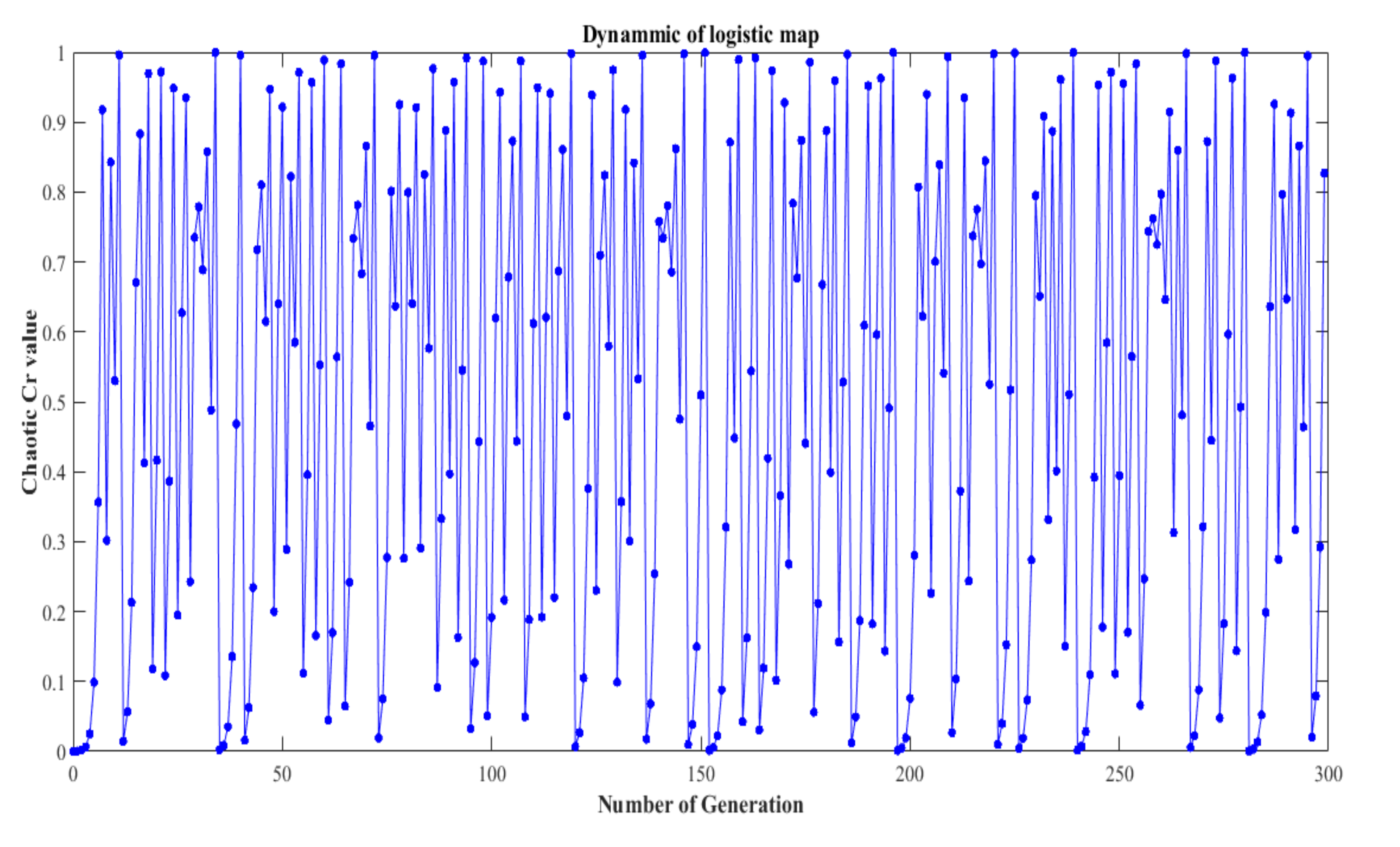
At the value of $\hspace{0.17em}\alpha =4$, Equation (42) outputs a chaotic sequence, having a value between 0 and 1. In Equation (42), for every independent run, $C{r}_0$ is generated randomly. Figure 1 depicts the chaotic value $Cr$ generated through a logistic map with $C{r}_0=0.001$ and 300 iterations.

For CPSO, the velocity update formula may be specified as:

$$v_{k+1}^{\left(i\right)}=w_k.v_k^{\left(i\right)}+c_1.C{r}_k.\left(G_{pk}^{\left(i\right)}-G_k^{\left(i\right)}\right)+c_2.\left(1-C{r}_k\right).\left(G_{gk}^{\left(i\right)}-G_k^{\left(i\right)}\right)$$

(44)

The following pseudo-code describes the computational process for calculating the domain of attraction in a polynomial system by using the proposed Chaotic-PSO-based algorithm.

Algorithm 2 Pseudo-code of the Chaotic-PSO

01: Start 02:   Initialise the particles swarm in a random way 03:   Create $C{r}_0$ randomly 04:   while (the ending criterion is not obtained or iteration number is performed) 05:    Assess the particle swarm fitness criterion 06:    for $p=1$ to particles’ number 07:     Determine $G_{pk}^{\left(i\right)}$ 08:     Determine $G_{gk}^{\left(i\right)}$ 09:     for $k=1$ till particle dimension number 10:      Refresh the chaotic $Cr$ value as described by Equation (42) 11:      Refresh the particles position as defined by Equations (37) and (38) 12:     Increment $k$ 13:    Increment $p$ 14:    Refresh the value of the inertia weight given by Equation (39) 15:   Increment generation till stopping criterion is satisfied 16:     end 17:     end 18:    end

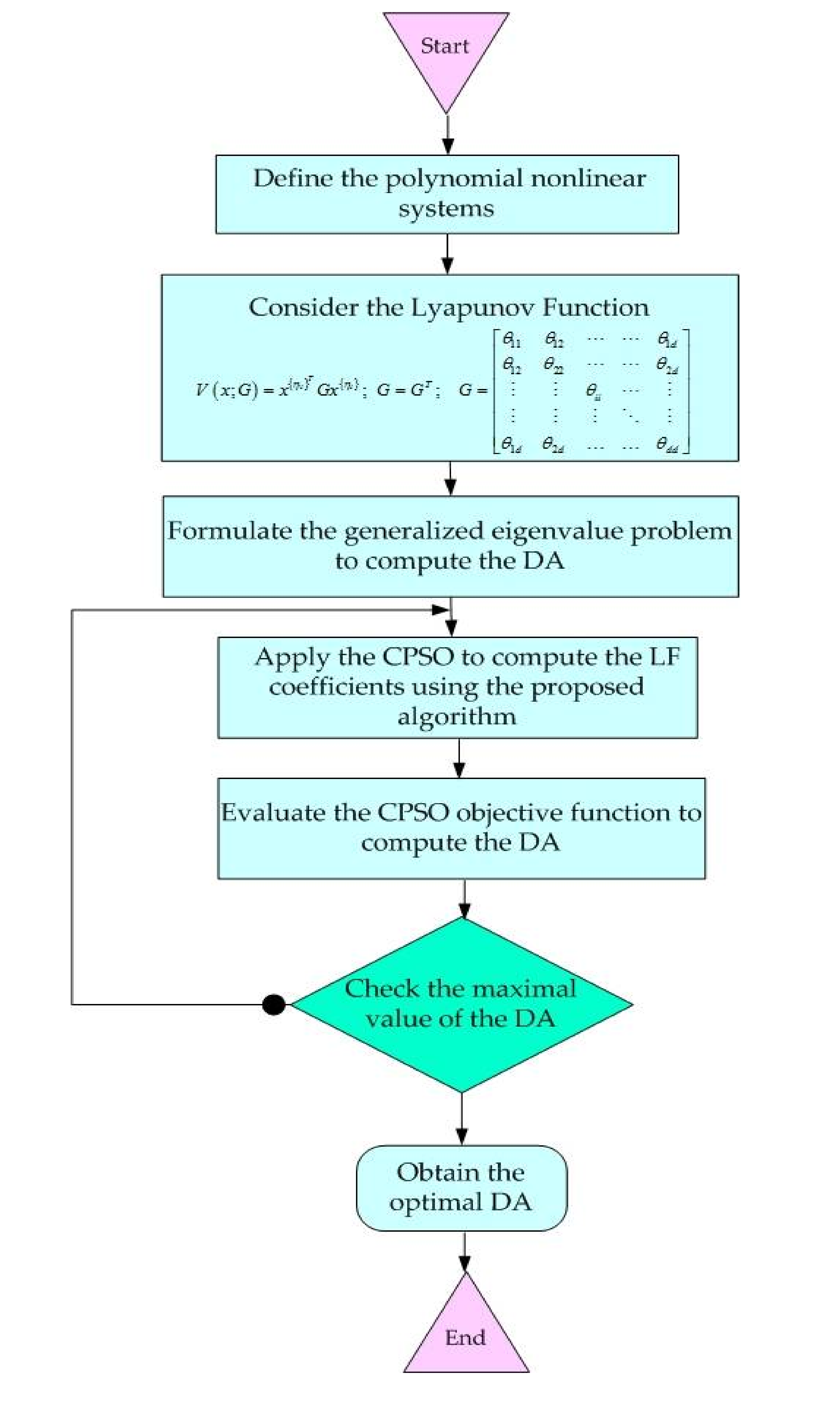
The flowchart describing the developed strategy is described by Figure 2.

5. Numerical Examples

In this section, we consider certain examples from previous research for which DA has been determined using Lyapunov quadratic functions to illustrate the effectiveness of the presented approach [10,26,39,40].

5.1. Example 1

Consider the Van der Pol equation’s state-space representation, given below [26].

$$\{\begin{array}{l}{\dot{x}}_1=-x_2\\ {\dot{x}}_2=x_1-x_2+x_1^2{x}_2\end{array}$$

(45)

The state vector here is represented by $x={\left[x_1\hspace{0.17em}{x}_2\right]}^T$. We employ the GEVP optimisation technique to estimate the initial DA of the steady equilibrium.

It is necessary to obtain a quadratic approximation of the asymptotic stability area around the origin. To achieve this, we examine the GEVP structure in (34) when the assigned Lyapunov function with degree ${\eta }_v=1$, which defines that the LEDA shape is chosen as

$$V\left(x\right)={\theta }_{11}{x}_1^2+2{\theta }_{12}{x}_1{x}_2+{\theta }_{22}{x}_2^2$$

(46)

This implies that $V\left(x;G\right)$ can be written using the SMR with regards to the vectors $x^{\left\{{\eta }_v\right\}}={\left[x_1,x_2\right]}^T$

$$V\left(x;G\right)=x^{{\left\{{\eta }_v\right\}}^T}G{x}^{\left\{{\eta }_v\right\}}=x^{{\left\{{\eta }_v\right\}}^T}\left[\begin{array}{cc}{\theta }_{11}& {\theta }_{12}\\ {\theta }_{12}& {\theta }_{22}\end{array}\right]x^{\left\{{\eta }_v\right\}}$$

(47)

To verify Theorem (2), let us use the polynomial

$$\dot{V}\left(x;G\right)=d_f\left(x\right)=\frac{\partial V\left(x;G\right)}{\partial x}f\left(x\right)$$

(48)

$$d_f\left(x\right)=2{\theta }_{12}{x}_1^2+2\left({\theta }_{22}-{\theta }_{12}-{\theta }_{11}\right)x_1{x}_2-2\left({\theta }_{12}+{\theta }_{22}\right)x_2^2+2{\theta }_{12}{x}_1^3{x}_2+2{\theta }_{22}{x}_1^2{x}_2^2$$

(49)

It is noteworthy that $D_f\left(\alpha ,G\right)$, indicating that the CSMR matrix of $d_f\left(x\right)$ is the corresponding vector of free variables.

$$D_f\left(\alpha ;G\right)=\left[\begin{array}{ccccc}2{\theta }_{12}& \left({\theta }_{22}-{\theta }_{12}-{\theta }_{11}\right)& 0& {\alpha }_1& {\alpha }_2\\ \left({\theta }_{22}-{\theta }_{12}-{\theta }_{11}\right)& -2\left({\theta }_{12}+{\theta }_{11}\right)& -{\alpha }_1& -{\alpha }_2& 0\\ 0& -{\alpha }_1& 0& {\theta }_{12}& {\alpha }_3\\ {\alpha }_1& -{\alpha }_2& {\theta }_{12}& {\theta }_{22}-2{\alpha }_3& 0\\ {\alpha }_2& 0& {\alpha }_3& 0& 0\end{array}\right]$$

(50)

where the free variables are computed with the values (8) and (12).

Let us note that the degree of $\dot{V}\left(x;G\right)$ is ${\eta }_d=4$. We can choose the degree of $e\left(x\right)$ as

$${\eta }_e\ge \frac{{\eta }_d}{2}-{\eta }_V$$

(51)

We select ${\eta }_e=1$

$$e\left(x\right)=e_{11}{x}_1^2+2e_{12}{x}_1{x}_2+e_{22}{x}_2^2$$

(52)

This implies that $e\left(x\right)$ can be written using the SMR with regards to the vectors $x^{\left\{{\eta }_e\right\}}={\left[x_1,x_2\right]}^T$

$$e\left(x\right)=x^{{\left\{{\eta }_e\right\}}^T}E{x}^{\left\{{\eta }_e\right\}}=x^{{\left\{{\eta }_e\right\}}^T}\left[\begin{array}{cc}{e}_{11}& e_{12}\\ e_{12}& e_{22}\end{array}\right]x^{\left\{{\eta }_e\right\}}$$

(53)

which implies ${\eta }_r={\eta }_v+{\eta }_s=2$. Vector $x^{\left\{{\eta }_r\right\}}$ is selected as $x^{\left\{{\eta }_r\right\}}={\left[x_1,x_2,x_1^2,x_1{x}_2,x_2^2\right]}^T$.

To calculate $Q\left(E,G\right)$ (Equation (31)) the SMR of the polynomial $Q\left(x,e\left(x\right),V\left(x;G\right)\right)\hspace{0.17em}\hspace{0.17em}$, we choose the matrix $K$ as

$$K=\left[\begin{array}{ccccc}1& 0& 0& 0& 0\\ 0& 1& 0& 0& 0\\ 0& 0& 1& 0& 0\\ 0& 0& 0& 1& 0\\ 0& 0& 0& 1& 0\\ 0& 0& 0& 0& 1\end{array}\right]$$

(54)

we obtain

$$Q\left(E,G\right)=\left[\begin{array}{ccccc}{e}_{11}& e_{12}& 0& 0& 0\\ e_{12}& e_{22}& 0& 0& 0\\ 0& 0& \mu {\theta }_{11}{e}_{11}& \mu \left({\theta }_{11}{e}_{12}-{\theta }_{12}{e}_{11}\right)& 0\\ 0& 0& \mu \left({\theta }_{11}{e}_{12}-{\theta }_{12}{e}_{11}\right)& \mu \left({\theta }_{11}{e}_{22}+4{\theta }_{12}{e}_{12}+{\theta }_{22}{e}_{11}\right)& \mu \left({\theta }_{22}{e}_{12}+{\theta }_{12}{e}_{22}\right)\\ 0& 0& 0& \mu \left({\theta }_{22}{e}_{12}+{\theta }_{12}{e}_{22}\right)& \mu {\theta }_{22}{e}_{22}\end{array}\right]$$

(55)

Lastly, we compute the $\tilde{Q}\left(E,G\right)$ SMR of the product $V\left(x;G\right)e\left(x\right)$

$$\tilde{Q}\left(E,G\right)=\left[\begin{array}{ccccc}0& 0& 0& 0& 0\\ 0& 0& 0& 0& 0\\ 0& 0& {\theta }_{11}{e}_{11}& \left({\theta }_{11}{e}_{12}-{\theta }_{12}{e}_{11}\right)& 0\\ 0& 0& \left({\theta }_{11}{e}_{12}-{\theta }_{12}{e}_{11}\right)& \left({\theta }_{11}{e}_{22}+4{\theta }_{12}{e}_{12}+{\theta }_{22}{e}_{11}\right)& \left({\theta }_{22}{e}_{12}+{\theta }_{12}{e}_{22}\right)\\ 0& 0& 0& \left({\theta }_{22}{e}_{12}+{\theta }_{12}{e}_{22}\right)& {\theta }_{22}{e}_{22}\end{array}\right]$$

(56)

For this purpose, we begin by encoding the variables to be determined as a position of every particle as per following matrix:

$$G^{\left(i\right)}=\left[\begin{array}{cc}{\theta }_{{}_{11}}^{\left(i\right)}& {\theta }_{{}_{12}}^{\left(i\right)}\\ {\theta }_{{}_{12}}^{\left(i\right)}& {\theta }_{{}_{22}}^{\left(i\right)}\end{array}\right],\hspace{0.17em}\hspace{0.17em}\hspace{0.17em}i=1,\dots ,p$$

(57)

The fitness value can be given by the maximum ${\gamma }^{*}$ for which there is a viable solution of the GEVP optimisation method as explained in the pseudo-code in Section 4.

The variables’ global optimisation $G_k^{\left(i\right)}$ is carried out by the CPSO operators, the location and the velocities.

The size of swarm is $p=50$ and the stopping condition is the highest number of iterations, $k_{\max }=100$.

To finish this step, by solving (34) with $\mu =0.1$ we get:

$$G^{*}=\left[\begin{array}{cc}1.1839& -0.4003\\ -0.4003& 0.8026\end{array}\right]$$

(58)

$$V\left(x\right)=1.1839x_1^2-0.8006x_1{x}_2+0.8026x_2^2$$

(59)

After solving this optimisation issue with $G^{*}$, we get the optimum domain of attraction as given below:

$$\vartheta \left(G^{*};\gamma \left(G^{*}\right)\right)=\left\{x\in {ℝ}^n:\hspace{0.17em}V\left(x\right)=1.1839x_1^2-0.8006x_1{x}_2+0.8026x_2^2=1.8770\right\}$$

(60)

The real value of the volume is:

$$\mathsf{\Omega }\left(G^{*}\right)=2.1118$$

(61)

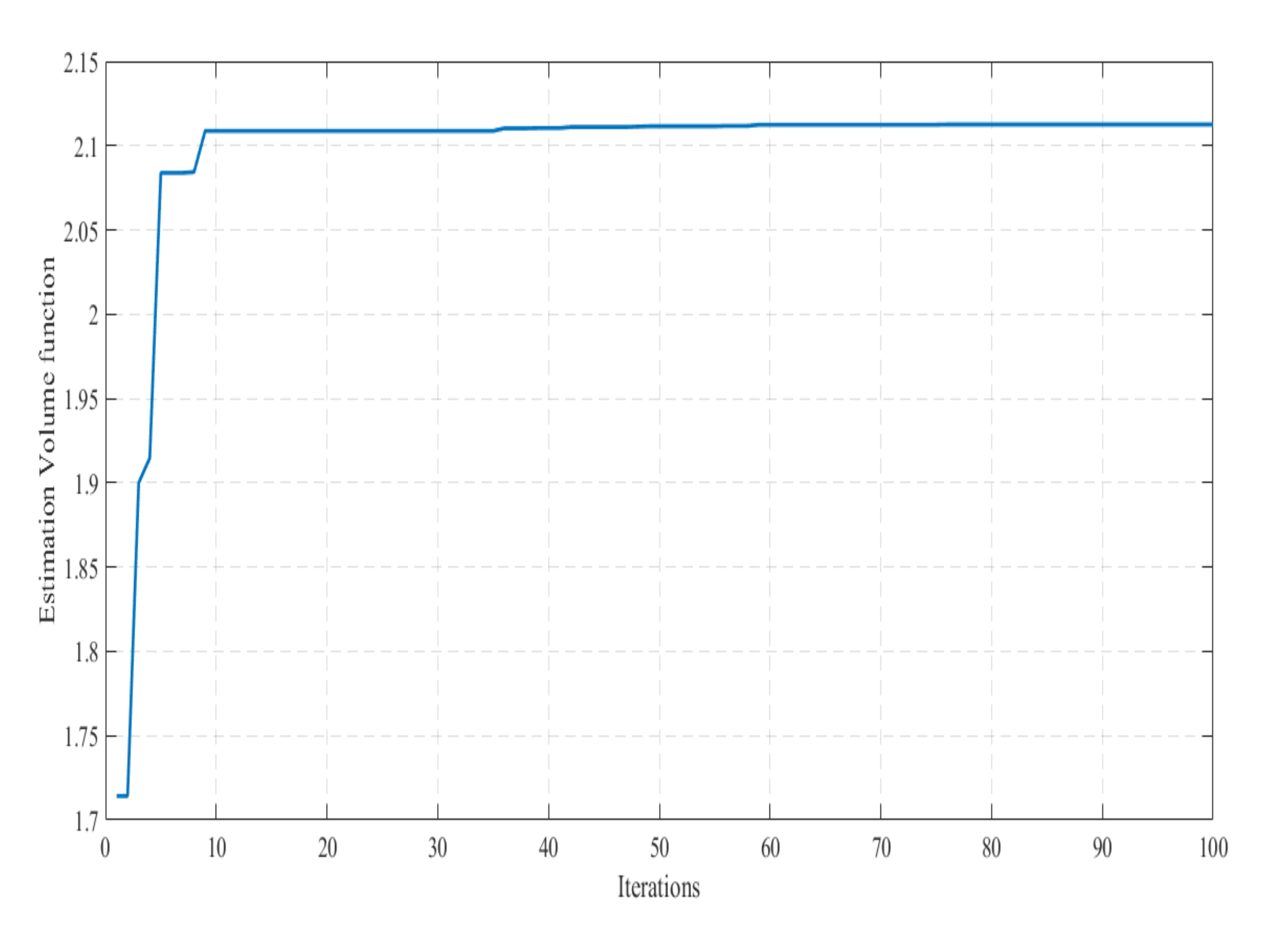
Figure 3 depicts the evolution of the CPSO process for 100 iterations. It can be clearly seen that the convergence of the algorithm takes place in less than 10 iterations. This shows the high performance of the developed method in computing the exact theoretical volume value $\mathsf{\Omega }\left(G^{*}\right)=2.1118$.

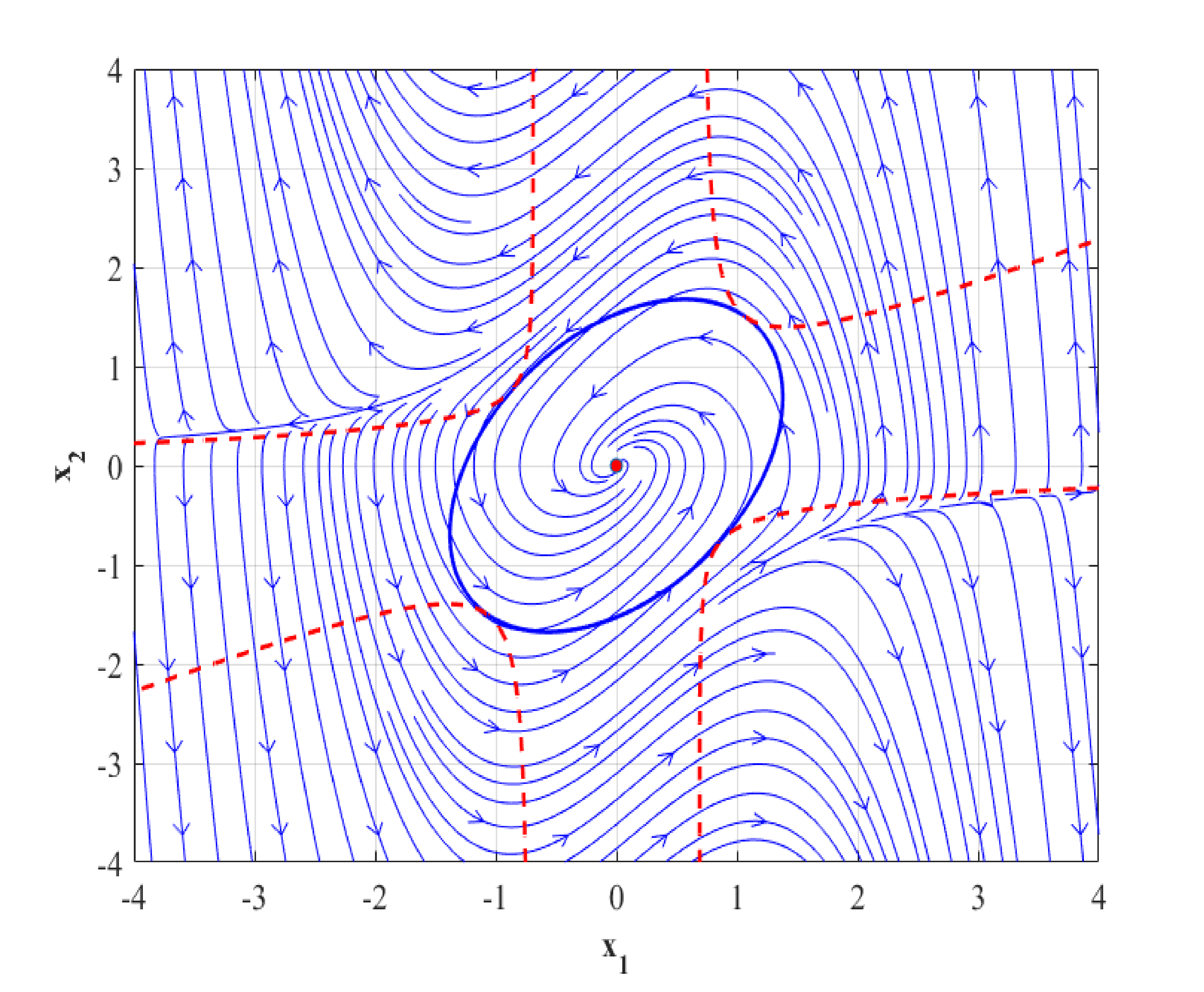
The above result, which provides the volume value $\mathsf{\Omega }\left(G^{*}\right)=2.1118$, helps obtain the largest estimated DA. This result is given by Figure 3. The approximated DA of the equilibrium with $\gamma \left(G^{*}\right)=1.8770$ is represented by the blue ellipsoid in Figure 4. However, the dashed red line, determines the boundary of the region where $\dot{V}\left(x,G^{*}\right)<0$.

Herein, one can accurately check the validity of the computed domain throughout the Lyapunov theory and its specified conditions.

5.2. Example 2

This instance is taken from Hahn [39]. It is necessary to find the "best" quadratic approximation of the stability area around the system’s origin. The system is as follows:

$$\{\begin{array}{l}{\dot{x}}_1=-x_1+2x_1^2{x}_2\\ {\dot{x}}_2=-x_2\end{array}$$

(62)

The precise stability area is known to be $x_1{x}_2<1$. In this area, the origin is depicted asymptotically. The LF describing the LEDA shape is chosen as

$$V\left(x;G\right)=x^{{\left\{{\eta }_v\right\}}^T}G{x}^{\left\{{\eta }_v\right\}}=x^{{\left\{{\eta }_v\right\}}^T}\left[\begin{array}{cc}{\theta }_{11}& {\theta }_{12}\\ {\theta }_{12}& {\theta }_{22}\end{array}\right]x^{\left\{{\eta }_v\right\}}$$

(63)

As the degree ${\eta }_d$ of $\dot{V}\left(x;G\right)$ amounts to 4, we can choose ${\eta }_e=1$ which entails ${\eta }_r=2$. Vectors $x^{\left\{{\eta }_e\right\}},\hspace{0.17em}\hspace{0.17em}{x}^{\left\{{\eta }_v\right\}}$ and $x^{\left\{{\eta }_r\right\}}$ are chosen as

$$\hspace{0.17em}{x}^{\left\{{\eta }_e\right\}}=\hspace{0.17em}{x}^{\left\{{\eta }_V\right\}}={\left[x_1,x_2\right]}^T,\hspace{0.17em}\hspace{0.17em}\hspace{0.17em}\hspace{0.17em}{x}^{\left\{{\eta }_r\right\}}={\left[x_1,x_2,x_1^2,x_1{x}_2,x_2^2\right]}^T$$

(64)

Thus,

$$D_f\left(\alpha ;G\right)=\left[\begin{array}{ccccc}-2{\theta }_{11}& -2{\theta }_{12}& 0& {\alpha }_1& {\alpha }_2\\ -2{\theta }_{12}& 2{\theta }_{22}& -{\alpha }_1& -{\alpha }_2& 0\\ 0& -{\alpha }_1& 0& 2{\theta }_{11}& {\alpha }_3\\ {\alpha }_1& -{\alpha }_2& 2{\theta }_{11}& 4{\theta }_{12}& 0\\ {\alpha }_2& 0& {\alpha }_3& 0& 0\end{array}\right]$$

(65)

$e\left(x\right)$ can be written using the SMR with regards to the vectors $x^{\left\{{\eta }_e\right\}}={\left[x_1,x_2\right]}^T$.

$$e\left(x\right)=x^{{\left\{{\eta }_e\right\}}^T}E{x}^{\left\{{\eta }_e\right\}}=x^{{\left\{{\eta }_e\right\}}^T}\left[\begin{array}{cc}{e}_{11}& e_{12}\\ e_{12}& e_{22}\end{array}\right]x^{\left\{{\eta }_e\right\}}$$

(66)

To compute $Q\left(E,G\right)$ (Equation (31)), the SMR of the polynomial $Q\left(x,e\left(x\right),V\left(x;G\right)\right)$. We select the matrix $K$ as

$$K=\left[\begin{array}{ccccc}1& 0& 0& 0& 0\\ 0& 1& 0& 0& 0\\ 0& 0& 1& 0& 0\\ 0& 0& 0& 1& 0\\ 0& 0& 0& 1& 0\\ 0& 0& 0& 0& 1\end{array}\right]$$

(67)

We obtain

$$Q\left(E,G\right)=\left[\begin{array}{ccccc}{e}_{11}& e_{12}& 0& 0& 0\\ e_{12}& e_{22}& 0& 0& 0\\ 0& 0& \mu {\theta }_{11}{e}_{11}& \mu \left({\theta }_{11}{e}_{12}-{\theta }_{12}{e}_{11}\right)& 0\\ 0& 0& \mu \left({\theta }_{11}{e}_{12}-{\theta }_{12}{e}_{11}\right)& \mu \left({\theta }_{11}{e}_{22}+4{\theta }_{12}{e}_{12}+{\theta }_{22}{e}_{11}\right)& \mu \left({\theta }_{22}{e}_{12}+{\theta }_{12}{e}_{22}\right)\\ 0& 0& 0& \mu \left({\theta }_{22}{e}_{12}+{\theta }_{12}{e}_{22}\right)& \mu {\theta }_{22}{e}_{22}\end{array}\right]$$

(68)

Finally, we compute the $\tilde{Q}\left(E,G\right)$ SMR of the product $V\left(x;G\right)e\left(x\right)$.

$$\tilde{Q}\left(E,G\right)=\left[\begin{array}{ccccc}0& 0& 0& 0& 0\\ 0& 0& 0& 0& 0\\ 0& 0& {\theta }_{11}{e}_{11}& \left({\theta }_{11}{e}_{12}-{\theta }_{12}{e}_{11}\right)& 0\\ 0& 0& \left({\theta }_{11}{e}_{12}-{\theta }_{12}{e}_{11}\right)& \left({\theta }_{11}{e}_{22}+4{\theta }_{12}{e}_{12}+{\theta }_{22}{e}_{11}\right)& \left({\theta }_{22}{e}_{12}+{\theta }_{12}{e}_{22}\right)\\ 0& 0& 0& \left({\theta }_{22}{e}_{12}+{\theta }_{12}{e}_{22}\right)& {\theta }_{22}{e}_{22}\end{array}\right]$$

(69)

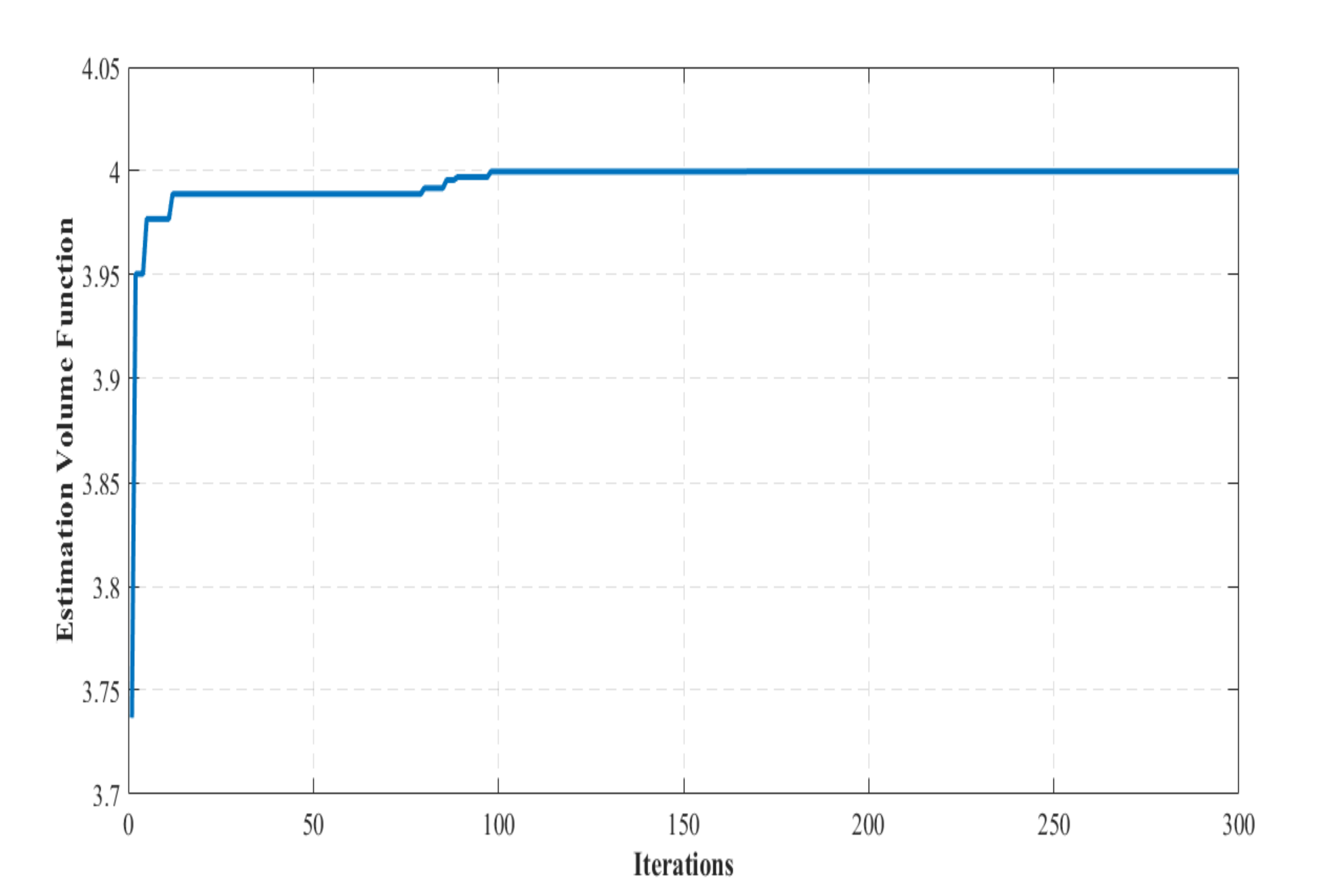
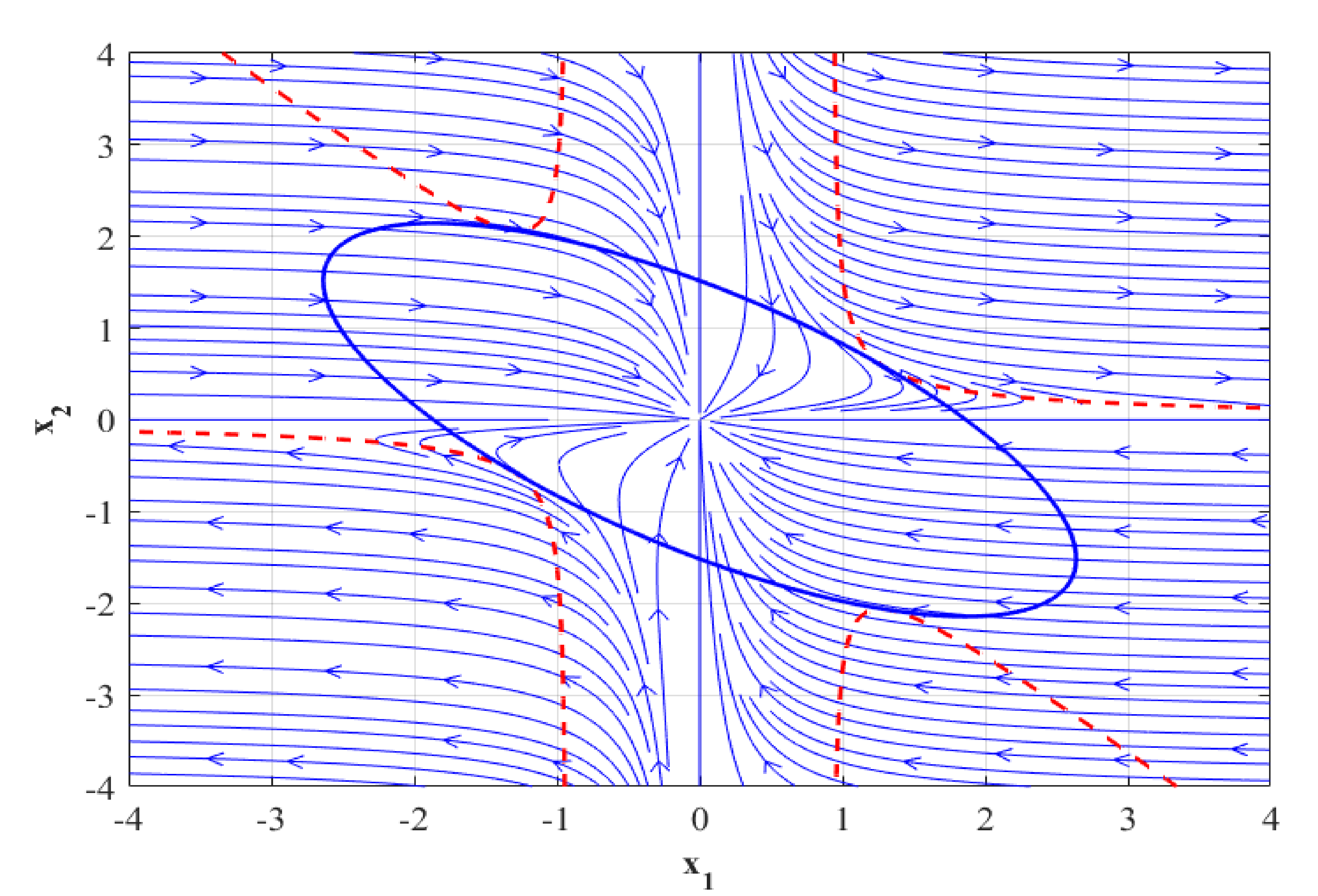
The dynamics of the synthesised optimisation algorithm is showed in Figure 5. Compared to the results presented in [39], this demonstrates the accuracy and swiftness of the CPSO technique established in this paper. Figure 6 describes the maximised DA of the equilibrium. The blue ellipsoid represents the DA estimate with $\gamma \left(G^{*}\right)=5.5715$, the dashed red line determines the boundary of the light blue area and represents the region in where $\stackrel{·}{V}\left(x\right)<0$. A high accuracy can be concluded regarding the obtained performance.

5.3. Example 3

The system in question is [40]:

$$\{\begin{array}{l}{\dot{x}}_1=-2x_1+x_3-x_2^3\\ {\dot{x}}_2=x_1-x_2-0.5x_1^3\\ {\dot{x}}_3=x_2-2x_3+0.5x_1^2\end{array}$$

(70)

Let us select $V\left(x;G\right)$ as

$$V\left(x;G\right)={\theta }_{11}{x}_1^2+2{\theta }_{12}{x}_1{x}_2+{\theta }_{22}{x}_2^2+2{\theta }_{13}{x}_1{x}_3+2{\theta }_{23}{x}_2{x}_3+{\theta }_{33}{x}_3^2$$

(71)

To consider the variables of concern for the matrix $G$, we reformulate the polynomial with its SMR as

$$V\left(x;G\right)=x^{{\left\{{\eta }_v\right\}}^T}G{x}^{\left\{{\eta }_v\right\}}$$

(72)

where

$$G=\left[\begin{array}{ccc}{\theta }_{11}& {\theta }_{12}& {\theta }_{13}\\ {\theta }_{12}& {\theta }_{22}& {\theta }_{23}\\ {\theta }_{13}& {\theta }_{23}& {\theta }_{33}\end{array}\right]$$

(73)

As the degree ${\eta }_d$ of $\dot{V}\left(x;G\right)$ amounts to 4, we can choose ${\eta }_e=1$ which entails ${\eta }_r=2$. Vectors $x^{\left\{{\eta }_e\right\}},\hspace{0.17em}\hspace{0.17em}{x}^{\left\{{\eta }_v\right\}}$ and $x^{\left\{{\eta }_r\right\}}$ are chosen as

$$\hspace{0.17em}{x}^{\left\{{\eta }_e\right\}}=\hspace{0.17em}{x}^{\left\{{\eta }_v\right\}}={\left[x_1,x_2,x_3\right]}^T,\hspace{0.17em}\hspace{0.17em}\hspace{0.17em}\hspace{0.17em}{x}^{\left\{{\eta }_r\right\}}={\left[x_1,x_2,x_3,x_1^2,x_1{x}_2,x_1{x}_3,x_2^2,x_2{x}_3,x_3^2\right]}^T$$

(74)

To verify Theorem (2), we introduce the drive Lyapunov function polynomial as

$$\dot{V}\left(x;G\right)=d_f\left(x\right)=\frac{\partial V\left(x;G\right)}{\partial x}f\left(x\right)$$

(75)

$$d_f\left(x\right)=2{\theta }_{12}{x}_1^2+2\left({\theta }_{22}-{\theta }_{12}-{\theta }_{11}\right)x_1{x}_2-2\left({\theta }_{12}+{\theta }_{22}\right)x_2^2+2{\theta }_{12}{x}_1^3{x}_2+2{\theta }_{22}{x}_1^2{x}_2^2$$

(76)

Then, the family of matrices $D_f\left(\alpha ,G\right)$ defining $d_f\left(x\right)$ can be configured affinely as

$$D_f\left(\alpha ,G\right)=D\left(G\right)+L\left(\alpha \right)$$

(77)

where $\alpha$ represents a vector of free variables and $L\left(\alpha \right)$ represents a linear parameterisation of $L$: Thus, the CSMR (complete SMR) of $d_f\left(x\right)$ is defined as

$$d_f\left(x\right)=x^{{\left\{{\eta }_v\right\}}^T}{D}_f\left(\alpha ,G\right)x^{\left\{{\eta }_v\right\}}$$

(78)

and $D_f\left(\alpha ,G\right)$ is known as CSMR matrix of $d_f\left(x\right)$. The quantities $\varsigma \left(n,{\eta }_r\right)$ and $\tau \left(n,{\eta }_r\right)$ are given, in that order, by (8) and (12).

Values of $\varsigma \left(n,{\eta }_r\right)$ and $\tau \left(n,{\eta }_r\right)$ for $n=3$ and ${\eta }_r=2$ are 14 and 20.

Thus,

$$D\left(G\right)=\left[\begin{array}{ccccccccc}-(2{\theta }_{11}-{\theta }_{12})& -(2{\theta }_{12}-{\theta }_{12}+{\theta }_{13})& -(4{\theta }_{13}-{\theta }_{11}-{\theta }_{23})& 0.5{\theta }_{13}& 0.5{\theta }_{23}& 0& 0.5{\theta }_{33}& 0& 0\\ -(2{\theta }_{12}-{\theta }_{12}+{\theta }_{13})& -2({\theta }_{22}-{\theta }_{23})& -(3{\theta }_{23}-{\theta }_{12}+{\theta }_{33})& 0& 0& 0& 0& 0& 0\\ -(4{\theta }_{13}-{\theta }_{11}-{\theta }_{23})& -(3{\theta }_{23}-{\theta }_{12}+{\theta }_{33})& 2({\theta }_{13}-2{\theta }_{33})& 0& 0& 0& 0& 0& 0\\ 0.5{\theta }_{13}& 0& 0& -{\theta }_{12}& -0.5{\theta }_{22}& 0& -0.5{\theta }_{23}& 0& 0\\ 0.5{\theta }_{23}& 0& 0& -0.5{\theta }_{22}& 0& {\theta }_{11}& 0& 0& 0\\ 0& 0& 0& 0& {\theta }_{11}& -2{\theta }_{12}& 0& -{\theta }_{13}& 0\\ 0.5{\theta }_{33}& 0& 0& -0.5{\theta }_{23}& 0& 0& 0& 0& 0\\ 0& 0& 0& 0& 0& -{\theta }_{13}& 0& 0& 0\\ 0& 0& 0& 0& 0& 0& 0& 0& 0\end{array}\right]$$

(79)

$$L\left(\alpha \right)=\left[\begin{array}{ccccccccc}0& 0& 0& {\alpha }_1& {\alpha }_2& {\alpha }_3& {\alpha }_4& {\alpha }_5& \left({\alpha }_6+{\alpha }_{18}\right)\\ 0& 0& -{\alpha }_1& -{\alpha }_2& 0& -\left({\alpha }_4+{\alpha }_7\right)& \left({\alpha }_{17}+{\alpha }_{20}\right)& -{\alpha }_6& {\alpha }_{19}\\ 0& -{\alpha }_1& 2{\alpha }_3& {\alpha }_7& -{\alpha }_{20}& 0& {\alpha }_8& \left({\alpha }_9+{\alpha }_{11}\right)& \left({\alpha }_{10}+{\alpha }_{12}\right)\\ {\alpha }_1& -{\alpha }_2& {\alpha }_7& -2\left({\alpha }_5+{\alpha }_{17}\right)& -{\alpha }_{18}& -{\alpha }_8& -{\alpha }_9& -{\alpha }_{10}& {\alpha }_{13}\\ {\alpha }_2& 0& -{\alpha }_{20}& -{\alpha }_{18}& -2{\alpha }_{19}& -{\alpha }_{11}& -{\alpha }_{12}& -{\alpha }_{13}& 0\\ {\alpha }_3& -\left({\alpha }_4+{\alpha }_7\right)& 0& -{\alpha }_8& -{\alpha }_{11}& 0& 0& {\alpha }_{14}& {\alpha }_{15}\\ {\alpha }_4& \left({\alpha }_{17}+{\alpha }_{20}\right)& {\alpha }_8& -{\alpha }_9& -{\alpha }_{12}& 0& -2{\alpha }_{14}& -{\alpha }_{15}& {\alpha }_{16}\\ {\alpha }_5& -{\alpha }_6& \left({\alpha }_9+{\alpha }_{11}\right)& -{\alpha }_{10}& -{\alpha }_{13}& {\alpha }_{14}& -{\alpha }_{15}& -2{\alpha }_{16}& 0\\ \left({\alpha }_6+{\alpha }_{18}\right)& {\alpha }_{19}& \left({\alpha }_{10}+{\alpha }_{12}\right)& {\alpha }_{13}& 0& {\alpha }_{15}& {\alpha }_{16}& 0& 0\end{array}\right]$$

(80)

To compute the SMR $Q\left(E,G\right)$ (Equation (31)) we calculate the polynomial $Q\left(x,e\left(x\right),V\left(x;G\right)\right)\hspace{0.17em}\hspace{0.17em}$

$$Q\left(x,e\left(x\right),G\right)\hspace{0.17em}\hspace{0.17em}=\left(1+\mu V\left(x,G\right)\right)e\left(x\right)$$

(81)

with

$$e\left(x\right)=e_1{x}_1^2+2e_2{x}_1{x}_2+e_3{x}_2^2+2e_4{x}_1{x}_3+2e_5{x}_2{x}_3+e_6{x}_3^2$$

(82)

This implies that $e\left(x\right)$ can be written using the SMR with regard to the vectors $x^{\left\{{\eta }_e\right\}}={\left[x_1,x_2,x_3\right]}^T$

$$e\left(x\right)=x^{{\left\{{\eta }_e\right\}}^T}E{x}^{\left\{{\eta }_e\right\}}=x^{{\left\{{\eta }_e\right\}}^T}\left[\begin{array}{ccc}{e}_1& e_2& e_4\\ e_2& e_3& e_5\\ e_4& e_5& e_6\end{array}\right]x^{\left\{{\eta }_e\right\}}$$

(83)

We obtain

$$\begin{array}{l}Q\left(x,e\left(x\right),G\right)\hspace{0.17em}\hspace{0.17em}=e_1{x}_1^2+2e_2{x}_1{x}_2+e_3{x}_2^2+2e_4{x}_1{x}_3+2e_5{x}_2{x}_3+e_6{x}_3^2+\mu {\theta }_{11}{e}_1{x}_1^4+2\mu \left({\theta }_{11}{e}_2+{\theta }_{12}{e}_1\right)x_1^3{x}_2\\ \hspace{0.17em}\hspace{0.17em}\hspace{0.17em}\hspace{0.17em}\hspace{0.17em}\hspace{0.17em}\hspace{0.17em}\hspace{0.17em}\hspace{0.17em}\hspace{0.17em}\hspace{0.17em}\hspace{0.17em}\hspace{0.17em}\hspace{0.17em}\hspace{0.17em}\hspace{0.17em}\hspace{0.17em}\hspace{0.17em}\hspace{0.17em}\hspace{0.17em}\hspace{0.17em}\hspace{0.17em}\hspace{0.17em}\hspace{0.17em}\hspace{0.17em}\hspace{0.17em}+\mu \left({\theta }_{11}{e}_3+4{\theta }_{12}{e}_2+{\theta }_{22}{e}_1\right)x_1^2{x}_2^2+2\mu \left({\theta }_{12}{e}_3+{\theta }_{22}{e}_2\right)x_1{x}_2^3+\mu {\theta }_{22}{e}_2{x}_2^4+2\mu \left({\theta }_{11}{e}_4+{\theta }_{13}{e}_1\right)x_1^3{x}_3\\ \hspace{0.17em}\hspace{0.17em}\hspace{0.17em}\hspace{0.17em}\hspace{0.17em}\hspace{0.17em}\hspace{0.17em}\hspace{0.17em}\hspace{0.17em}\hspace{0.17em}\hspace{0.17em}\hspace{0.17em}\hspace{0.17em}\hspace{0.17em}\hspace{0.17em}\hspace{0.17em}\hspace{0.17em}\hspace{0.17em}\hspace{0.17em}\hspace{0.17em}\hspace{0.17em}\hspace{0.17em}\hspace{0.17em}\hspace{0.17em}\hspace{0.17em}\hspace{0.17em}+\mu \left(4{\theta }_{13}{e}_4+{\theta }_{33}{e}_1+{\theta }_{11}{e}_6\right)x_1^2{x}_2^3+2\mu \left({\theta }_{12}{e}_3+{\theta }_{22}{e}_2+{\theta }_{13}{e}_6+{\theta }_{33}{e}_4\right)x_1{x}_3^3\hspace{0.17em}\hspace{0.17em}+\mu {\theta }_{33}{e}_6{x}_3^4\\ \hspace{0.17em}\hspace{0.17em}\hspace{0.17em}\hspace{0.17em}\hspace{0.17em}\hspace{0.17em}\hspace{0.17em}\hspace{0.17em}\hspace{0.17em}\hspace{0.17em}\hspace{0.17em}\hspace{0.17em}\hspace{0.17em}\hspace{0.17em}\hspace{0.17em}\hspace{0.17em}\hspace{0.17em}\hspace{0.17em}\hspace{0.17em}\hspace{0.17em}\hspace{0.17em}\hspace{0.17em}\hspace{0.17em}\hspace{0.17em}\hspace{0.17em}\hspace{0.17em}+2\mu \left({\theta }_{11}{e}_5+2{\theta }_{12}{e}_4+2{\theta }_{13}{e}_2+{\theta }_{23}{e}_1\right)x_1^2{x}_2{x}_3+2\mu \left(2{\theta }_{12}{e}_5+{\theta }_{22}{e}_4+{\theta }_{13}{e}_3+2{\theta }_{23}{e}_2\right)x_1{x}_2^2{x}_3\\ \hspace{0.17em}\hspace{0.17em}\hspace{0.17em}\hspace{0.17em}\hspace{0.17em}\hspace{0.17em}\hspace{0.17em}\hspace{0.17em}\hspace{0.17em}\hspace{0.17em}\hspace{0.17em}\hspace{0.17em}\hspace{0.17em}\hspace{0.17em}\hspace{0.17em}\hspace{0.17em}\hspace{0.17em}\hspace{0.17em}\hspace{0.17em}\hspace{0.17em}\hspace{0.17em}\hspace{0.17em}\hspace{0.17em}\hspace{0.17em}\hspace{0.17em}\hspace{0.17em}+2\mu \left({\theta }_{12}{e}_6+2{\theta }_{13}{e}_5+{\theta }_{23}{e}_4+{\theta }_{33}{e}_2\right)x_1{x}_2{x}_3^2+\mu \left(2{\theta }_{22}{e}_5+2{\theta }_{23}{e}_3+{\theta }_{33}{e}_2\right)x_2^3{x}_3\\ \hspace{0.17em}\hspace{0.17em}\hspace{0.17em}\hspace{0.17em}\hspace{0.17em}\hspace{0.17em}\hspace{0.17em}\hspace{0.17em}\hspace{0.17em}\hspace{0.17em}\hspace{0.17em}\hspace{0.17em}\hspace{0.17em}\hspace{0.17em}\hspace{0.17em}\hspace{0.17em}\hspace{0.17em}\hspace{0.17em}\hspace{0.17em}\hspace{0.17em}\hspace{0.17em}\hspace{0.17em}\hspace{0.17em}\hspace{0.17em}\hspace{0.17em}\hspace{0.17em}+\mu \left({\theta }_{22}{e}_6+2{\theta }_{23}{e}_3+{\theta }_{33}{e}_3\right)x_2^2{x}_3^2+2\mu \left({\theta }_{23}{e}_6+{\theta }_{33}{e}_5\right)x_2{x}_3^3\end{array}$$

(84)

The SMR of the polynomial $Q\left(x,e\left(x\right),G\right)\hspace{0.17em}\hspace{0.17em}$

$$Q\left(E,G\right)=\left[\begin{array}{ccccccccc}{e}_1& e_2& e_4& 0& 0& 0& 0& 0& 0\\ e_2& e_3& e_5& 0& 0& 0& 0& 0& 0\\ e_4& e_5& e_6& 0& 0& 0& 0& 0& 0\\ 0& 0& 0& \mu {\theta }_{11}{e}_1& \mu \left({\theta }_{11}{e}_2+{\theta }_{12}{e}_1\right)& 0& \mu \left({\theta }_{11}{e}_4+{\theta }_{13}{e}_1\right)& m_1& 0\\ 0& 0& 0& \mu \left({\theta }_{11}{e}_2+{\theta }_{12}{e}_1\right)& m_4& \mu \left({\theta }_{12}{e}_3+{\theta }_{22}{e}_2\right)& 0& m_2& m_3\\ 0& 0& 0& 0& \mu \left({\theta }_{12}{e}_3+{\theta }_{22}{e}_2\right)& \mu {\theta }_{22}{e}_2& 0& m_5& 0\\ 0& 0& 0& \mu \left({\theta }_{11}{e}_4+{\theta }_{13}{e}_1\right)& 0& 0& m_6& 0& m_7\\ 0& 0& 0& m_1& m_2& m_5& 0& m_8& \mu \left({\theta }_{23}{e}_6+{\theta }_{33}{e}_5\right)\\ 0& 0& 0& 0& m_3& 0& m_7& \mu \left({\theta }_{23}{e}_6+{\theta }_{33}{e}_5\right)& \mu {\theta }_{33}{e}_6\end{array}\right]$$

(85)

with

$$\begin{array}{l}{m}_1=\mu \left({\theta }_{11}{e}_5+2{\theta }_{12}{e}_4+2{\theta }_{13}{e}_2+{\theta }_{23}{e}_1\right),\hspace{0.17em}\hspace{0.17em}{m}_2=\mu \left(2{\theta }_{12}{e}_5+{\theta }_{22}{e}_4+{\theta }_{13}{e}_3+2{\theta }_{23}{e}_2\right),\hspace{0.17em}\hspace{0.17em}{m}_3=\mu \left({\theta }_{12}{e}_6+2{\theta }_{13}{e}_5+{\theta }_{23}{e}_4+{\theta }_{33}{e}_2\right)\\ m_4=\mu \left({\theta }_{11}{e}_3+4{\theta }_{12}{e}_2+{\theta }_{22}{e}_1\right),\hspace{0.17em}\hspace{0.17em}{m}_5=0.5\mu \left(2{\theta }_{22}{e}_5+2{\theta }_{23}{e}_3+{\theta }_{33}{e}_2\right),\hspace{0.17em}{m}_6=\mu \left(4{\theta }_{13}{e}_4+{\theta }_{33}{e}_1+{\theta }_{11}{e}_6\right)\\ m_7=\mu \left({\theta }_{12}{e}_3+{\theta }_{22}{e}_2+{\theta }_{13}{e}_6+{\theta }_{33}{e}_4\right),\hspace{0.17em}\hspace{0.17em}{m}_8=\mu \left({\theta }_{22}{e}_6+2{\theta }_{23}{e}_3+{\theta }_{33}{e}_3\right)\end{array}$$

(86)

Finally, we compute the polynomial $\tilde{Q}\left(x,e\left(x\right),G\right)=V\left(x;G\right)e\left(x\right)$.

$$\begin{array}{l}\tilde{Q}\left(x,e\left(x\right),G\right)\hspace{0.17em}\hspace{0.17em}={\theta }_{11}{e}_1{x}_1^4+2\left({\theta }_{11}{e}_2+{\theta }_{12}{e}_1\right)x_1^3{x}_2+\left({\theta }_{11}{e}_3+4{\theta }_{12}{e}_2+{\theta }_{22}{e}_1\right)x_1^2{x}_2^2\\ \hspace{0.17em}\hspace{0.17em}\hspace{0.17em}\hspace{0.17em}\hspace{0.17em}\hspace{0.17em}\hspace{0.17em}\hspace{0.17em}\hspace{0.17em}\hspace{0.17em}\hspace{0.17em}\hspace{0.17em}\hspace{0.17em}\hspace{0.17em}+2\left({\theta }_{12}{e}_3+{\theta }_{22}{e}_2\right)x_1{x}_2^3+{\theta }_{22}{e}_2{x}_2^4+2\left({\theta }_{11}{e}_4+{\theta }_{13}{e}_1\right)x_1^3{x}_3+\left(4{\theta }_{13}{e}_4+{\theta }_{33}{e}_1+{\theta }_{11}{e}_6\right)x_1^2{x}_2^3\\ \hspace{0.17em}\hspace{0.17em}\hspace{0.17em}\hspace{0.17em}\hspace{0.17em}\hspace{0.17em}\hspace{0.17em}\hspace{0.17em}\hspace{0.17em}\hspace{0.17em}\hspace{0.17em}\hspace{0.17em}\hspace{0.17em}\hspace{0.17em}+2\left({\theta }_{12}{e}_3+{\theta }_{22}{e}_2+{\theta }_{13}{e}_6+{\theta }_{33}{e}_4\right)x_1{x}_3^3\hspace{0.17em}\hspace{0.17em}+{\theta }_{33}{e}_6{x}_3^4\\ \hspace{0.17em}\hspace{0.17em}\hspace{0.17em}\hspace{0.17em}\hspace{0.17em}\hspace{0.17em}\hspace{0.17em}\hspace{0.17em}\hspace{0.17em}\hspace{0.17em}\hspace{0.17em}\hspace{0.17em}\hspace{0.17em}\hspace{0.17em}+2\left({\theta }_{11}{e}_5+2{\theta }_{12}{e}_4+2{\theta }_{13}{e}_2+{\theta }_{23}{e}_1\right)x_1^2{x}_2{x}_3+2\left(2{\theta }_{12}{e}_5+{\theta }_{22}{e}_4+{\theta }_{13}{e}_3+2{\theta }_{23}{e}_2\right)x_1{x}_2^2{x}_3\\ \hspace{0.17em}\hspace{0.17em}\hspace{0.17em}\hspace{0.17em}\hspace{0.17em}\hspace{0.17em}\hspace{0.17em}\hspace{0.17em}\hspace{0.17em}\hspace{0.17em}\hspace{0.17em}\hspace{0.17em}\hspace{0.17em}\hspace{0.17em}+2\left({\theta }_{12}{e}_6+2{\theta }_{13}{e}_5+{\theta }_{23}{e}_4+{\theta }_{33}{e}_2\right)x_1{x}_2{x}_3^2+\left(2{\theta }_{22}{e}_5+2{\theta }_{23}{e}_3+{\theta }_{33}{e}_2\right)x_2^3{x}_3\\ \hspace{0.17em}\hspace{0.17em}\hspace{0.17em}\hspace{0.17em}\hspace{0.17em}\hspace{0.17em}\hspace{0.17em}\hspace{0.17em}\hspace{0.17em}\hspace{0.17em}\hspace{0.17em}\hspace{0.17em}\hspace{0.17em}\hspace{0.17em}+\left({\theta }_{22}{e}_6+2{\theta }_{23}{e}_3+{\theta }_{33}{e}_3\right)x_2^2{x}_3^2+2\left({\theta }_{23}{e}_6+{\theta }_{33}{e}_5\right)x_2{x}_3^3\end{array}$$

(87)

The SMR of the product $\tilde{Q}\left(E,G\right)$

$$\tilde{Q}\left(E,G\right)=\left[\begin{array}{ccccccccc}0& 0& 0& 0& 0& 0& 0& 0& 0\\ 0& 0& 0& 0& 0& 0& 0& 0& 0\\ 0& 0& 0& 0& 0& 0& 0& 0& 0\\ 0& 0& 0& {\theta }_{11}{e}_1& \left({\theta }_{11}{e}_2+{\theta }_{12}{e}_1\right)& 0& \mu \left({\theta }_{11}{e}_4+{\theta }_{13}{e}_1\right)& \frac{1}{\mu }{m}_1& 0\\ 0& 0& 0& \left({\theta }_{11}{e}_2+{\theta }_{12}{e}_1\right)& \frac{1}{\mu }{m}_4& \left({\theta }_{12}{e}_3+{\theta }_{22}{e}_2\right)& 0& \frac{1}{\mu }{m}_2& \frac{1}{\mu }{m}_3\\ 0& 0& 0& 0& \left({\theta }_{12}{e}_3+{\theta }_{22}{e}_2\right)& {\theta }_{22}{e}_2& 0& \frac{1}{\mu }{m}_5& 0\\ 0& 0& 0& \left({\theta }_{11}{e}_4+{\theta }_{13}{e}_1\right)& 0& 0& m_6& 0& m_7\\ 0& 0& 0& \frac{1}{\mu }{m}_1& \frac{1}{\mu }{m}_2& \frac{1}{\mu }{m}_5& 0& m_8& \left({\theta }_{23}{e}_6+{\theta }_{33}{e}_5\right)\\ 0& 0& 0& 0& m_3& 0& m_7& \left({\theta }_{23}{e}_6+{\theta }_{33}{e}_5\right)& {\theta }_{33}{e}_6\end{array}\right]$$

(88)

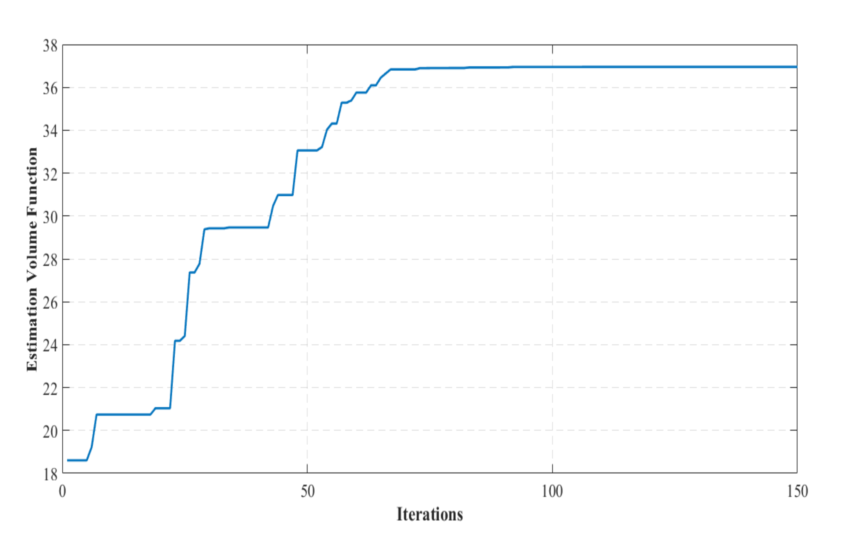
In Figure 7 and Figure 8, it is straightforward to check the direct convergence of the algorithm. Indeed, no further fluctuation can be observed, which makes it possible to minimise the convergence time. The steady-state dynamic of the estimated volume is therefore reached after around 65 iterations. A small number of approaches in the literature have studied this kind of system. The technique developed in this paper shows its superiority in providing the maximal volume value in shorter computation time.

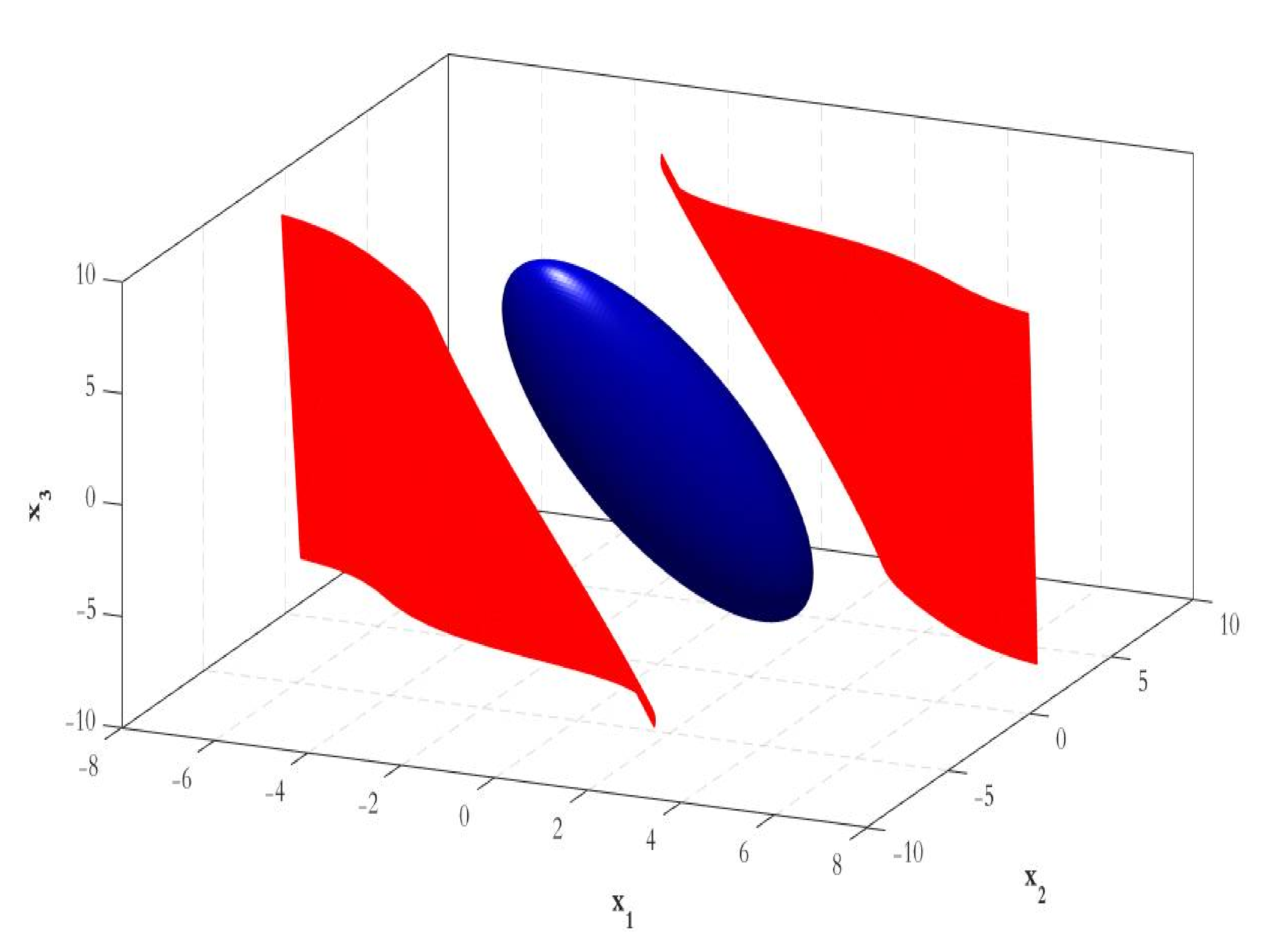
Figure 8 shows the validity of the obtained DA. Nevertheless, it is theoretically possible to further increase the estimated DA. As a direct explanation for this fact, it can be noted that the obtained domain is not maximal due to the selected LF. The optimal computing of the LF constitutes one of the most advantageous aspects of this work.

6. Results Analysis and Discussion

This section is dedicated to an evaluative comparative analysis between the synthesised CPSO estimation strategy in this paper and another peer reviewed technique [26].

Table 1. Benchmark nonlinear systems using defined quadratic LF calculated with the proposed CSPO algorithm in this paper.

Example	Systems Dynamic	Lyapunov Function CPSO	Domain Radius CPSO $\mathit{\gamma }\left({\mathit{G}}^{*}\right)$	Domain Volume CPSO $\sqrt{\frac{{\left(\mathit{\gamma }\left({\mathit{G}}^{*}\right)\right)}^{\mathit{n}}}{\mathbf{det}\left({\mathit{G}}^{*}\right)}}$
E1 [39,40]	$\{\begin{array}{l}{\dot{x}}_1=-x_2\\ {\dot{x}}_2=x_1-x_2+x_1^2{x}_2\end{array}$	$V\left(x\right)=1.1839x_1^2-0.8006x_1{x}_2+0.8026x_2^2$	1.8770	2.1118
E2 [39,40]	$\{\begin{array}{l}{\dot{x}}_1=-x_1+2x_1^2{x}_2\\ {\dot{x}}_2=-x_2\end{array}$	$V\left(x\right)=1.6024x_1^2+2.7862x_1{x}_2+2.4222x_2^2$	5.5715	4.000
E3 [39]	$\{\begin{array}{l}{\dot{x}}_1=-2x_1+x_3-x_2^3\\ {\dot{x}}_2=x_1-x_2-\frac{1}{2}{x}_1^3\\ {\dot{x}}_3=x_2-2x_3+\frac{1}{2}{x}_1^2\end{array}$	$\begin{array}{l}V\left(x;G\right)=0.8349x_1^2+0.178x_1{x}_2+x_2^2\\ \hspace{0.17em}\hspace{0.17em}\hspace{0.17em}\hspace{0.17em}\hspace{0.17em}\hspace{0.17em}\hspace{0.17em}\hspace{0.17em}\hspace{0.17em}\hspace{0.17em}\hspace{0.17em}\hspace{0.17em}\hspace{0.17em}\hspace{0.17em}\hspace{0.17em}\hspace{0.17em}\hspace{0.17em}\hspace{0.17em}\hspace{0.17em}\hspace{0.17em}\hspace{0.17em}\hspace{0.17em}+0.2588x_1{x}_3+0.0477x_2{x}_3\\ \hspace{0.17em}\hspace{0.17em}\hspace{0.17em}\hspace{0.17em}\hspace{0.17em}\hspace{0.17em}\hspace{0.17em}\hspace{0.17em}\hspace{0.17em}\hspace{0.17em}\hspace{0.17em}\hspace{0.17em}\hspace{0.17em}\hspace{0.17em}\hspace{0.17em}\hspace{0.17em}\hspace{0.17em}\hspace{0.17em}\hspace{0.17em}\hspace{0.17em}\hspace{0.17em}\hspace{0.17em}\hspace{0.17em}+0.1610x_3^2\end{array}$	4.4916	36.9241

provides the estimated DA features for three dynamical nonlinear systems with quadratic LF(s) taken from the literature [39,40]. The selected examples are presented in their nonlinear polynomial form. Examples E1 [39] and E2 [40] are second-order systems. However, example E3 [39] is a third-order nonlinear polynomial model. Please note that the main evaluation criterion is the domain volume. The obtained results are quite satisfactory in terms of the value of the domain volume. Moreover, the designed strategy provides a complete solution starting from defining the optimal LF and finishing with providing the maximal domain volume. This result is achieved for all studied examples with an easy implementation concept and low consuming time.

A second step was performed to evaluate the performance of the CPSO strategy, consisting of investigating the domain volume for the three examples based on the same LF that was reported in [26,39,40].

For each example, the maximum possible value of $\mathsf{\Omega }\left(G^{*}\right)$ is computed by the CPSO method and compared with the outcomes obtained by a peer optimisation-based technique, reported in the literature [26]. It appears obvious in

Table 2. Comparative analysis with benchmark nonlinear systems using a defined quadratic LF as described in [39,40].

Example.	Systems Dynamic	Lyapunov Function	Domain Radius [26] $\mathit{\gamma }\left({\mathit{G}}^{*}\right)$	Domain Volume [26] $\sqrt{\frac{{\left(\mathit{\gamma }\left({\mathit{G}}^{*}\right)\right)}^{\mathit{n}}}{\mathbf{det}\left({\mathit{G}}^{*}\right)}}$	Domain Radius CPSO $\mathit{\gamma }\left({\mathit{G}}^{*}\right)$	Domain Volume CPSO $\sqrt{\frac{{\left(\mathit{\gamma }\left({\mathit{G}}^{*}\right)\right)}^{\mathit{n}}}{\mathbf{det}\left({\mathit{G}}^{*}\right)}}$
E1 [39,40]	$\{\begin{array}{l}{\dot{x}}_1=-x_2\\ {\dot{x}}_2=x_1-x_2+x_1^2{x}_2\end{array}$	$V\left(x\right)=1.5x_1^2-0.5x_1{x}_2+x_2^2$	2.3180	2.0733	2.4197	2.1642
E2 [39,40]	$\{\begin{array}{l}{\dot{x}}_1=-x_1+2x_1^2{x}_2\\ {\dot{x}}_2=-x_2\end{array}$	$V\left(x\right)=0.33x_1^2+0.249x_1{x}_2+0.376x_2^2$	1.000	4.000	1.000	4.000
E3 [39,40]	$\begin{array}{l}\{\begin{array}{l}{\dot{x}}_1=-2x_1+x_3-x_2^3\\ {\dot{x}}_2=x_1-x_2-\frac{1}{2}{x}_1^3\\ {\dot{x}}_3=x_2-2x_3+\frac{1}{2}{x}_1^2\end{array}\\ \end{array}$	$\begin{array}{l}V\left(x;G\right)=0.2742x_1^2+0.3634x_1{x}_2\\ \hspace{0.17em}\hspace{0.17em}\hspace{0.17em}\hspace{0.17em}\hspace{0.17em}\hspace{0.17em}\hspace{0.17em}\hspace{0.17em}\hspace{0.17em}\hspace{0.17em}\hspace{0.17em}+0.4578x_2^2+0.1820x_1{x}_3\\ \hspace{0.17em}\hspace{0.17em}\hspace{0.17em}\hspace{0.17em}\hspace{0.17em}\hspace{0.17em}\hspace{0.17em}\hspace{0.17em}\hspace{0.17em}\hspace{0.17em}\hspace{0.17em}+0.1892x_2{x}_3+0.1077x_3^2\end{array}$	$\le 1$	$\le 12.0849$	1.0246	12.5328

that for the three investigated examples, the estimated volumes of the DA(s) attained by the CPSO technique are significantly better than the estimates resulting from optimisation-based approaches. For the case of example E3, the performance of the CPSO scheme is even larger and more accurate.

Likewise, it can be concluded that the developed CPSO procedure is appropriate for estimating enlarged DA of polynomial nonlinear systems. As a matter of fact, it is computationally operational and converges to the optimal DA estimate in a significantly reduced time. Despite the benefit of offering more accurate DA in less time, CPSO can be very useful for real-time control problems. It is likewise valuable for control strategies that use online sequential composition formalism as described in [26]. Finally, we should emphasise the fact that the work presented in [26] is based on a random procedure that characterises the evolution of the designed algorithm. This means that an intensive simulation study should be performed each time to obtain the optimal solutions. This fact is the main disadvantage for the described approach. For the CPSO strategy, the final estimated domain is the same independent of the simulation settings.

7. Conclusions

This paper studies the quadratic Lyapunov function calculation, which expands the DA volume estimate for systems with polynomials. The designed scheme presented in this paper has the main objective of computing an optimal LF so as to search the largest sublevel set of the DA. Iterative methods based on CPSO were established to obtain the LEDA lower bound. By leveraging CPSO capacity, a new enhanced PSO by using chaotic maps for global optimisation and encoding the variables of the quadratic Lyapunov function to be determined as particle positions was presented. The main advantage of the established algorithm is that one can evaluate the necessary and sufficient conditions as stated in Lyapunov theory with respect to initial conditions selected for the system state variables. The outcomes of the simulations substantiated that the parameters chosen using CPSO possibly leads to the biggest DA. Moreover, no trade-off between the algorithm computational cost and convergence speed is imposed. The convergence rate is therefore reduced, favouring the online implementation for trajectory tracking purposes of complex nonlinear dynamical systems or hybrid nonlinear systems.

Motivated by the excellent outcomes obtained for the instances that were employed, the designed methodology can be considered for other kinds of nonlinear systems and for real processes, which by definition possess nonlinearities. Consideration of the case of rational LF is also a beneficial aspect to this work.

References

1. Khalil, H.K. Nonlinear Systems, 3rd ed.; Prentice Hall: Upper Saddle River, NJ, USA, 2002. [Google Scholar]
2. Jerbi, H. Estimations of the Domains of Attraction for Classes of Nonlinear Continuous Polynomial Systems. Arab. J. Sci. Eng. 2017, 42, 2829–2837. [Google Scholar] [CrossRef]
3. Jerbi, H.M.; Hamidi, F.; Ben Aoun, S.; Olteanu, S.C.; Popescu, D. Lyapunov-based Methods for Maximizing the Domain of Attraction. Int. J. Comput. Commun. Control 2020, 15, 5. [Google Scholar] [CrossRef]
4. Jerbi, H.; Braiek, N.B.; Bacha, A.B.B. A Method of Estimating the Domain of Attraction for Nonlinear Discrete-Time Systems. Arab. J. Sci. Eng. 2014, 39, 3841–3849. [Google Scholar] [CrossRef]
5. Hamidi, F.; Jerbi, H. A Synthesis on Lyapunov Methods to the Estimation and Enlargement of Attraction Domain for Nonlinear Autonomous Systems. In Proceedings of the 2009 International Conference on Computational Intelligence, Modelling and Simulation, Brno, Czech Republic, 7–9 September 2009; pp. 87–92. [Google Scholar]
6. Hamidi, F.; Jerbi, H.; Aggoune, W.; Djemai, M.; Abdelkrim, M.N. Enlarging the Domain of Attraction in Nonlinear Polynomial Systems. Int. J. Comput. Commun. Control 2013, 8, 538. [Google Scholar] [CrossRef] [Green Version]
7. Hamidi, F.; Abdelkrim, M.N.; Houssem, J. Searching Candidate Lyapunov Function with Threshold Accepting Algorithm. In Proceedings of the 2011 Third International Conference on Computational Intelligence, Communication Systems and Networks, Bali, Indonesia, 26–28 July 2011; pp. 26–31. [Google Scholar]
8. Chesi, G.; Garulli, A.; Tesi, A.; Vicino, A. LMI-based computation of optimal quadratic Lyapunov functions for odd polynomial systems. Int. J. Rob. Nonlinear Control 2004, 15, 35–49. [Google Scholar] [CrossRef]
9. Hamidi, F.; Jerbi, H.; Aggoune, W.; Djemai, M.; Abdkrim, M.N. Enlarging region of attraction via LMI-based approach and Genetic Algorithm. In Proceedings of the 2011 International Conference on Communications, Computing and Control Applications (CCCA), Hammamet, Tunisia, 3–5 March 2011; pp. 1–6. [Google Scholar]
10. Hachicho, O. A novel LMI-based optimization algorithm for the guaranteed estimation of the domain of attraction using rational Lyapunov functions. J. Frankl. Inst. 2007, 344, 535–552. [Google Scholar] [CrossRef]
11. Hamidi, F.; Jerbi, H.; Olteanu, S.C.; Popescu, D. An Enhanced Stabilizing Strategy for Switched Nonlinear Systems. Stud. Inform. Control 2019, 28, 391–400. [Google Scholar] [CrossRef]
12. Chakrabarty, A.; Danielson, C.; Di Cairano, S.; Raghunathan, A. Active learning for estimating reachable sets for systems with unknown dynamics. IEEE Trans. Cybern. 2020, 1–12. [Google Scholar] [CrossRef]
13. Chesi, G. Estimating the domain of attraction for uncertain polynomial systems. Automatica 2004, 40, 1981–1986. [Google Scholar] [CrossRef]
14. Dubljević, S.; Kazantzis, N. A new Lyapunov design approach for nonlinear systems based on Zubov’s method. Automatica 2002, 38, 1999–2007. [Google Scholar] [CrossRef]
15. Rozgonyi, S.; Hangos, K.; Szederkényi, G. Determining the domain of attraction of hybrid non-linear systems using maximal Lyapunov functions. Kybernetika 2010, 46, 19–37. [Google Scholar]
16. Loccufier, M.; Noldus, E. A New Trajectory Reversing Method for Estimating Stability Regions of Autonomous Nonlinear Systems. Nonlinear Dyn. 2000, 21, 265–288. [Google Scholar] [CrossRef]
17. Chesi, G.; Garulli, A.; Tesi, A.; Vicino, A. Robust analysis of LFR systems through homogeneous polynomial Lyapunov functions. IEEE Trans. Autom. Control 2004, 49, 1211–1215. [Google Scholar] [CrossRef]
18. Lam, H.-K.; Seneviratne, L. BMI-based stability and performance design for fuzzy-model-based control systems subject to parameter uncertainties. IEEE Trans. Syst. Man Cybern. 2007, 37, 502–514. [Google Scholar] [CrossRef]
19. Topcu, U.; Packard, A.; Seiler, P. Local stability analysis using simulations and sum-of-squares programming. Automatica 2008, 44, 2669–2675. [Google Scholar] [CrossRef]
20. Han, D.; Panagou, D. Chebyshev approximation and higher order derivatives of Lyapunov functions for estimating the domain of attraction. In Proceedings of the 2017 IEEE 56th Annual Conference on Decision and Control (CDC), Melbourne, VIC, Australia, 12–15 December 2017; pp. 1181–1186. [Google Scholar]
21. Popescu, D.; Dauphin-Tanguy, G.; Foulloy, L. Modelisation, Identification et Commande des Systemes; Romanian Academy Press: Bucharest, Romania, 2004; ISBN 973-27-1086-1. [Google Scholar]
22. Mone, M.-A.; Diop, S.; Popescu, D. Optimal Control for Diesel Engine Combustion Regime. In Proceedings of the 2019 22nd International Conference on Control Systems and Computer Science (CSCS), Bucharest, Romania, 8–30 May 2019; pp. 42–47. [Google Scholar]
23. Chesi, G.; Garulli, A.; Tesi, A.; Vicino, A. Solving quadratic distance problems: An LMI-based approach. IEEE Trans. Autom. Control 2003, 48, 200–212. [Google Scholar] [CrossRef]
24. Chesi, G. Computing Output Feedback Controllers to Enlarge the Domain of Attraction in Polynomial Systems. IEEE Trans. Autom. Control 2004, 49, 1846–1850. [Google Scholar] [CrossRef]
25. Chuang, L.-Y.; Tsai, S.-W.; Yang, C.-H. Chaotic catfish particle swarm optimization for solving global numerical optimization problems. Appl. Math. Comput. 2011, 217, 6900–6916. [Google Scholar] [CrossRef]
26. Najafi, E.; Babuška, R.; Lopes, G. A fast sampling method for estimating the domain of attraction. Nonlinear Dyn. 2016, 86, 823–834. [Google Scholar] [CrossRef] [Green Version]
27. Peška, L.; Tashu, T.M.; Horváth, T. Swarm intelligence techniques in recommender systems—A review of recent research. Swarm Evol. Comput. 2019, 48, 201–219. [Google Scholar] [CrossRef]
28. Zhang, Y.; Wang, S.; Ji, G. A Comprehensive Survey on Particle Swarm Optimization Algorithm and Its Applications. Math. Probl. Eng. 2015, 2015, 1–38. [Google Scholar] [CrossRef] [Green Version]
29. Del Ser, J.; Osaba, E.; Molina, D.; Yang, X.S.; Salcedo-Sanz, S.; Camacho, D.; Herrera, F. Bio-inspired computation: Where we stand and what’s next. Swarm Evol. Comput. 2019, 48, 220–250. [Google Scholar] [CrossRef]
30. Boubaker, S.; Djemai, M.; Manamanni, N.; M’Sahli, F. Active modes and switching instants identification for linear switched systems based on Discrete Particle Swarm Optimization. Appl. Soft Comput. 2014, 14, 482–488. [Google Scholar] [CrossRef]
31. Park, S.; Song, N.; Yu, W.; Kim, D. PSR: PSO-Based Signomial Regression Model. Int. J. Fuzzy Log. Intell. Syst. 2019, 19, 307–314. [Google Scholar] [CrossRef] [Green Version]
32. Poli, R.; Kennedy, J.; Blackwell, T. Particle swarm optimization. Swarm Intell. 2007, 1, 33–57. [Google Scholar] [CrossRef]
33. Bergh, F.V.D.; Engelbrecht, A.P. A study of particle swarm optimization particle trajectories. Inf. Sci. 2006, 176, 937–971. [Google Scholar]
34. Clerc, M.; Kennedy, J. The particle swarm—Explosion, stability, and convergence in a multidimensional complex space. IEEE Trans. Evol. Comput. 2002, 6, 58–73. [Google Scholar] [CrossRef] [Green Version]
35. Del Valle, Y.; Venayagamoorthy, G.K.; Mohagheghi, S.; Hernandez, J.-C.; Harley, R.G. Particle Swarm Optimization: Basic Concepts, Variants and Applications in Power Systems. IEEE Trans. Evol. Comput. 2008, 12, 171–195. [Google Scholar] [CrossRef]
36. Ran, M.; Wang, Q.; Dong, C.; Ni, M. Multistage anti-windup design for linear systems with saturation nonlinearity: Enlargement of the domain of attraction. Nonlinear Dyn. 2015, 80, 1543–1555. [Google Scholar] [CrossRef]
37. Trelea, I.C. The particle swarm optimization algorithm: Convergence analysis and parameter selection. Inf. Process. Lett. 2003, 85, 317–325. [Google Scholar] [CrossRef]
38. Shi, Y.; Eberhart, R.C. Empirical study of particle swarm optimization. In Proceedings of the 1999 Congress on Evolutionary Computation-CEC99, Washington, DC, USA, 6–9 July 2003; pp. 1945–1949. [Google Scholar]
39. Davison, E.; Kurak, E. A computational method for determining quadratic lyapunov functions for non-linear systems. Automatica 1971, 7, 627–636. [Google Scholar] [CrossRef]
40. Chesi, G. Estimating the domain of attraction via union of continuous families of Lyapunov estimates. Syst. Control Lett. 2007, 56, 326–333. [Google Scholar] [CrossRef]
Figure 1. Chaotic Cr value using a logic map.
Electronics 09 01704 g001
Figure 2. Flowchart of the CPSO method for estimating the attraction domain.
Electronics 09 01704 g002
Figure 3. Evolution of Ω ( G ) using CPSO method for the Van der Pol example.
Electronics 09 01704 g003
Figure 4. Approximated DA for the Van der Pol model in the CPSO method; the blue ellipsoid characterises the estimated stability domain, the (the boundary of the light blue area) dashed red line denotes the region in which V · ( x ) < 0 .
Electronics 09 01704 g004
Figure 5. Evolution of Ω ( G ) using CPSO method for the Hahn model.
Electronics 09 01704 g005
Figure 6. Approximated DA for the Hahn model with CPSO method. Blue ellipsoid represents the DA estimate, red dashed line (the boundary of the DA estimate) represents the region in which V · ( x ) < 0 .
Electronics 09 01704 g006
Figure 7. Evolution of Ω ( G ) using CPSO method for the three-dimension example.
Electronics 09 01704 g007
Figure 8. Approximated DA for the CPSO method; the blue ellipsoid represents the DA estimate, the blue surface (the boundary of the light red area) represents the region in which V · ( x ) < 0 .
Electronics 09 01704 g008