A Systolic Accelerator for Neuromorphic Visual Recognition

Abstract

Advances in neuroscience have encouraged researchers to focus on developing computational models that behave like the human brain. HMAX is one of the potential biologically inspired models that mimic the primate visual cortex’s functions and structures. HMAX has shown its effectiveness and versatility in multi-class object recognition with a simple computational structure. It is still a challenge to implement the HMAX model in embedded systems due to the heaviest computational S2 phase of HMAX. Previous implementations such as CoRe16 have used a reconfigurable two-dimensional processing element (PE) array to speed up the S2 layer for HMAX. However, the adder tree mechanism in CoRe16 used to produce output pixels by accumulating partial sums in different PEs increases the runtime for HMAX. To speed up the execution process of the S2 layer in HMAX, in this paper, we propose SAFA (systolic accelerator for HMAX), a systolic-array based architecture to compute and accelerate the S2 stage of HMAX. Using the output stationary (OS) dataflow, each PE in SAFA not only calculates the output pixel independently without additional accumulation of partial sums in multiple PEs, but also reduces the multiplexers applied in reconfigurable accelerators. Besides, data forwarding for the same input or weight data in OS reduces the memory bandwidth requirements. The simulation results show that the runtime of the heaviest computational S2 stage in HMAX model is decreased by 5.7%, and the bandwidth required for memory is reduced by 3.53 × on average by different kernel sizes (except for kernel = 12) compared with CoRe16. SAFA also obtains lower power and area costs than other reconfigurable accelerators from synthesis on ASIC.

1. Introduction

The human brain is the most power-efficient processor. The last three decades have seen great success in understanding the ventral and dorsal pathways for the human visual cortex. These advances have motivated computer vision scientists to develop so-called “neuromorphic vision algorithms” for perception and cognition [1,2,3,4]. Neuromorphic models have shown high computing power and impressive performances with simple neural structures via reverse-engineering of the human brain.

Among them, hierarchical model and X (HMAX) [5] is one of the potential primate cortical models. HMAX was first proposed by Riesenhuber and Poggio in 1999 [5] and later extended by Serre et al. in 2007 [6]. It is a feedforward hierarchical feature model for object recognition tasks with a simple computation structure. HMAX can achieve an excellent balance between the computation cost, simplicity, and recognition performance, which benefits the embedded and low-power systems. Thus, HMAX has attracted many researchers to improve its performance or to accelerate the computation process [7,8,9,10,11,12].

HMAX mainly consists of four processing stages (S1, C1, S2, C2) with a hierarchy of alternating S (convolutional) and C (pooling) layers by progressively integrating inputs from the lower layers. Among the four stages, the S2 layer is the most computing-intensive. This stage convolutes each scale of C1 layer with a large number of convolution kernels. The computation complexity for S2 layer is O ($k^{2}r{M}^2{P}_i$), where $k\times k$ is the kernel size, r indicates the number of orientation, $M\times M$ is the size of the input C1 layer, and $P_i$ ($i~4000$) is the number of weight patches. Cortical Network Simulator (CNS) [13] for HMAX on GPU also indicates that HMAX spends nearly 85% of the total runtime to compute the S2 features.

Therefore, it is still a significant challenge to deploy the HMAX model on real-time artificial intelligence at the edge. Fortunately, lots of work has been investigated to accelerate the S2 layer of HMAX [11,14,15]. Sabarad et al. [11] composed processing element (PE) arrays to form a reconfigurable two-dimensional convolution accelerator CoRe16 on FPGA to accelerate the heaviest computational S2 layer of HMAX model. Experimental results show that it achieves great speedup increased by 5 to 15 times compared to CNS-based implementation. Park et al. [15] used a different reconfigurable PE array to accelerate the S2 layer of HMAX. However, the adder tree mechanism in CoRe16, Park et al., and Maashri et al. [14], used to calculate each output pixel by accumulation of partial sums in different PEs, lowers the execution speed for HMAX.

To further speed up the execution process of S2 layer in HMAX, in this paper, we propose SAFA (systolic accelerator for HMAX), a systolic-array based accelerator for the S2 stage in HMAX model. Systolic arrays perform high computational parallelism by communicating directly between large numbers of relatively simple, identical PE arrays [16]. Work in [17] indicates that output stationary (OS) dataflow in systolic array runs faster than input stationary (IS) or weight stationary (WS) dataflow. We then use the OS dataflow [18] to accelerate the S2 computation process for SAFA. Each PE in SAFA produces an output pixel independently without additional accumulation of partial sums in multiple PEs like CoRe16, which increases the calculation speed. Differently from the traditional PE, which executes multiplication and accumulation (MAC) in the systolic array, our designed PE uses a Gaussian radial basis function (GRBF) [19] operation for the S2 layer in HMAX. Following OS dataflow, our PE also lessens the multiplexers used in SAFA, and so can attain low power and area costs compared with reconfigurable accelerators. Besides, data forwarding for the same input or weight data in one cycle for OS dataflow reduces the required memory bandwidth. The main contributions are as follows:

1. We propose a systolic convolution array for the HMAX model, which can calculate different sizes of convolution.

2. We utilize the OS dataflow to compute each output pixel in every PE independently, which speeds up the execution process of the S2 layer in HMAX. Our designed PE can not only match the computation for the S2 layer in HMAX, but also reduces the multiplexers used in SAFA, which helps to obtain low power and area costs. Meanwhile, data forwarding for the same input feature map or weight parameters in SAFA greatly reduces the memory bandwidth requirement for SAFA.

3. We compared the runtime of SAFA with different shapes and found the best form of the systolic array to accelerate the S2 layer in HMAX. The simulation results show that the most computationally-intensive S2 phase’s runtime is decreased by 5.7%, and the storage bandwidth is reduced by 3.53 times on average for different kernel sizes (except for kernel = 12) compared with CoRe16. The synthesis results of SAFA on ASIC also achieve lower power and area costs than reconfigurable accelerators such as CoRe16.

The rest of our work is organized as follows. Section 2 presents the background and preliminary information. In Section 3, we introduce the structure of SAFA, the PE function, and the dataflow for SAFA in detail. Simulation results and discussions compared with CoRe16 and other reconfigurable accelerators are given in Section 4. Finally, we conclude this paper in Section 5.

2. Background and Preliminary Information

The HMAX model we utilize in this paper was extended by Serre et al. [6]. As shown in Figure 1, the HMAX model [6] is a four-stage (S1, C1, S2, C2) feature extraction model which follows the hierarchical layer by alternating convolutional template matching (S1 and S2 layers) and max pooling operations (C1 and C2 layers). The overall goal of HMAX model is to transform the gray scale images into feature vectors, which can be issued to a support vector machine (SVM) for the final classification. The detailed computation process of HMAX is as follows.

S1 layer: The gray value input image is first convolved by Gabor filters in the S1 layer with different orientations at every possible position. As shown in

Table 1. Summary of the S1 and C1 layer parameters. The filter sizes of S1 layer range from $7\times 7$ to $37\times 37$ with a step size of 2, leading to 64 different receptive fields in total (4 orientations × 16 scales). C1 layer pooling sizes spread from $8\times 8$ to $22\times 22$ with a step size of 2 corresponding to the S1 layer scale bands.

Scale Band	C1 Spatial Pooling Grid	Overlap	S1 Filter Size
Band 1	$8\times 8$	4	$7\times 7$ $9\times 9$
Band 2	$10\times 10$	5	$11\times 11$ $13\times 13$
Band 3	$12\times 12$	6	$15\times 15$ $17\times 17$
Band 4	$14\times 14$	7	$19\times 19$ $21\times 21$
Band 5	$16\times 16$	8	$23\times 23$ $25\times 25$
Band 6	$18\times 18$	9	$27\times 27$ $29\times 29$
Band 7	$20\times 20$	10	$31\times 31$ $33\times 33$
Band 8	$22\times 22$	11	$35\times 35$ $37\times 37$

, the filter sizes in the S1 layer range from $7\times 7$ to $37\times 37$ with a step size of two pixels (only four scales are visualized in Figure 1). Thus, the S1 layer has 64 different receptive fields (4 orientations × 16 scales) used for convolution.

C1 layer: The C1 layer is the first max pooling layer to pool over nearby two S1 scales with the same orientation to the scale band. This operation also subsamples the S1 features, leading to a smaller C1 layer size while maintaining the same number of orientations as the S1 layer. The pooling units spread from $8\times 8$ to $22\times 22$ with a step size of two for the corresponding scale bands in S1 layer. Note that the C1 responses are not calculated at every possible location, and the C1 layer only overlaps by an amount from 4 to 11 with a step size of 1 (Table 1) corresponding to different scale bands in S1 layer. This also makes the computations in the next layer more efficient.

S2 layer: The S2 features are computed by template matching each position and scale bands of the C1 layer (referred as $X_s$) with a dictionary of predefined patches ($P_i$). Each $P_i$ prototype kernel is of size $n\times n\times r$, where n ∈ {4, 8, 12, 16} and r denote the orientation. The following GRBF [19] gives the response of S2:

$$\begin{array}{c}\hfill R\left(X_s,P_i\right)=exp(-\frac{{∥X_s-P_i∥}^2}{2\alpha {\sigma }^2}),\end{array}$$

(1)

where $X_{s=\left\{1,\dots 4\right\}}$ represents the number of scale bands in C1 layer, and $P_{i=\left\{1\dots 4000\right\}}$ indicates the number of prototype kernels in the dictionary. We set $\alpha$ = ${\left(n/4\right)}^2$, and the standard deviation $\sigma$ is 1, the same as CoRe16 [11]. The S2 output can be $P_i$ ($i~4000$) group feature maps depending on the number of $P_i$.

C2 layer: The C2 response is calculated by a global max pooling over all scales and positions of each S2 type to obtain a single vector. Each S2 type corresponds to the match for every prototype $P_i$ and the input image at every position and scale. The C2 response $R_{C2}$ is expressed as

$$\begin{array}{c}\hfill R_{C2}=max\left\{R\left(X_s,P_i\right)\right\}.\end{array}$$

(2)

To implement S2 and C2 computation in hardware, alternatively, the S2 and C2 calculations can be re-formulated as

$$\begin{array}{c}\hfill R\left(X_s,P_i\right)=\frac{{∥X_s-P_i∥}^2}{2\alpha {\sigma }^2},\end{array}$$

(3)

$$\begin{array}{c}\hfill R_{C2}=exp\left\{min\left\{R\left(X_s,P_i\right)\right\}\right\}.\end{array}$$

(4)

This reformulation indicates that the exponential operation of S2 calculation can be moved to after the C2 layer to reduce the number of exponential functions. Consequently, the C2 layer operation is global minimum rather than a global maximum and we merely need to conduct an exponential operation on the reduced data (Equation (3)) once to obtain C2 vectors. Similarly, we can also calculate the constant denominator term $\alpha$ in Equation (3) for a given $P_i$ kernel size. This helps reduce computing resources (multipliers) for the S2 layer, which in turn is used to accelerate convolution operations. Above all, we only need to compute the Euclidean distance between the C1 input and the patches (${∥X_s-P_i∥}^2$) after reformulation to accelerate the S2 process in hardware.

3. SAFA: Systolic Accelerator for HMAX

In this section, we introduce the accelerator architecture: SAFA (systolic accelerator for HMAX) to accelerate the S2 computation for HMAX. Our S2 layer of HMAX accelerator SAFA is made up of systolic arrays with highly modular space and temporal regularity.

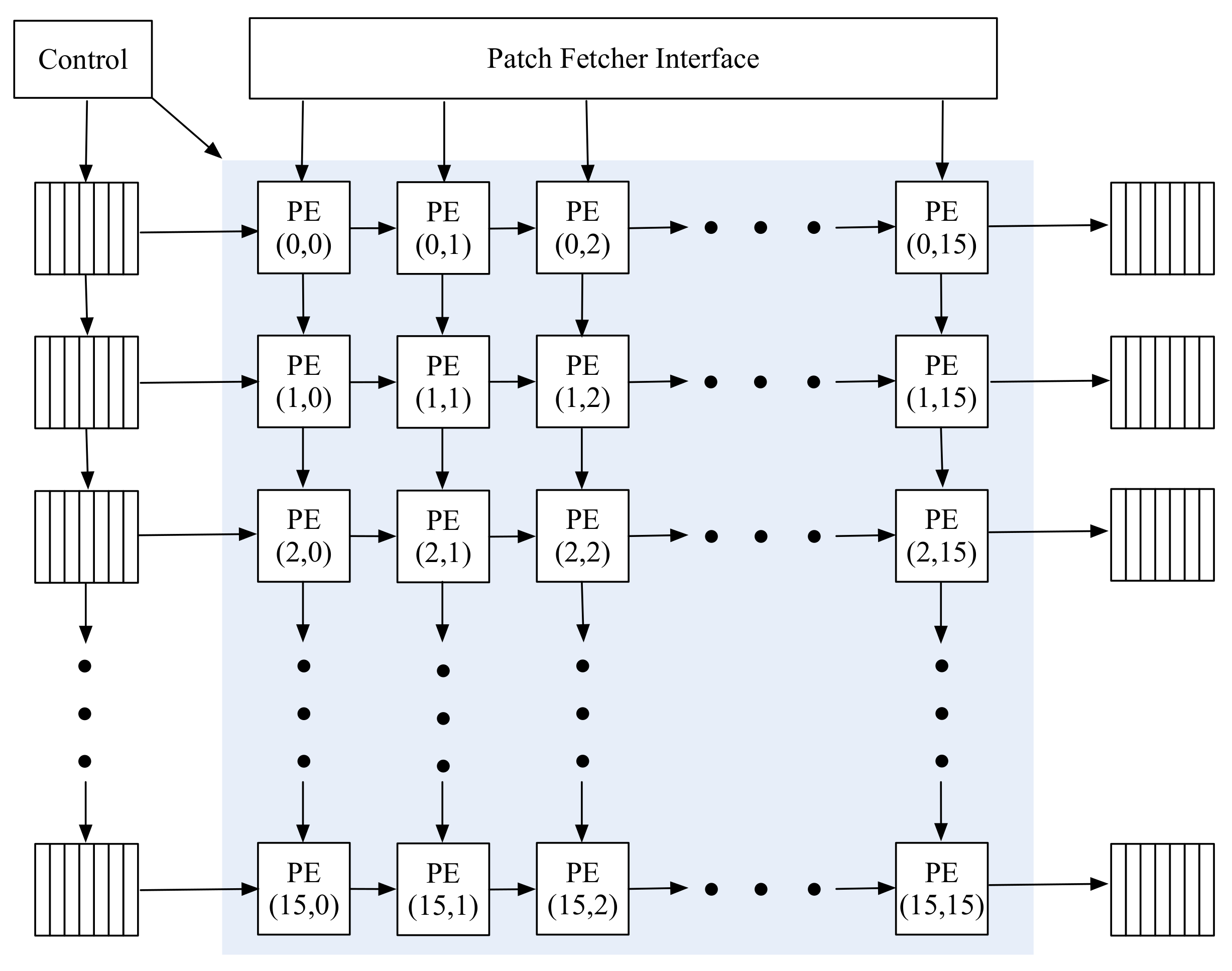
3.1. Structure of the Systolic Array

As shown in Figure 2, SAFA is a $16\times 16$ systolic array that contains 256 identical and simple PEs. The global and large fan-out interconnect is divided into local interconnections between neighboring PEs. Besides, the input/output data are transferred into/from the PE array between the neighboring PEs to avoid the use of redundant multiplexers. Combined with the short, local, peer-to-peer interconnects, SAFA can obtain a high frequency with massive parallelization over even a thousand PEs.

3.2. Processing Element

The processing element we design is the fundamental computational element in SAFA. Figure 3 shows the schematic diagram of our designed PE. The PE includes three calculation components and four registers. The activation register passes C1 input data to the right neighbor PE and the patch register passes the S2 patch to the down PE. The subtractor is followed by a multiplier to calculate the partial sum of the Euclidean distance between the C1 feature and the patch parameter. The adder then accumulates this partial sum. The control register dominates the accumulated times. It depends on the size of $P_i$ kernel and orientation, ensuring that each PE computes one output pixel of S2 layer. Once the current PE figures out one output pixel, a register will transfer it to the right neighbor PE.

Differently from the traditional systolic array where the PE performs MAC operation, our designed PE implements subtraction, multiplication, and accumulation operations to carry out the reduced GRBF [19] function in S2 layer (details are illustrated in Section 2). Compared with reconfigurable accelerators, such as CoRe16 or Park et al. [15], our PE also does not use the multiplexers or other selectors to choose the available C1 layer input or patches. This also reduces the computational resource and helps to decrease the computing power for SAFA.

3.3. Schematic Dataflow for SAFA

Figure 4 depicts the schematic dataflow for SAFA. We mainly utilize the OS dataflow for SAFA. Assume the input C1 feature map is of size $M\times M\times r$; then the output S2 feature map for each $P_i$ is of size $(M-n+1)\times (M-n+1)\times r$. We mainly use the HMAX model extended by reference [6] in this paper. It is a classic implementation of HMAX model which exhibits an excellent balance between recognition performance and computation cost for many different object categories.

A larger orientation value r, larger kernel size n, and larger number of patches $P_i$ can improve the accuracy of the HMAX. Reference [6] indicates that when the orientation equals four, kernel size is four, and with $P_i$ being 400, HMAX can provide enough performance for object classification. Considering the performance and simplicity, we set the orientation as four—kernel size being four—and the number of patches to 400 in this paper, as shown in Figure 3. Besides, we use the same input image size $256\times 256$ as CoRe16 [11]. The S1 layer size is similar to the input image since the S1 layer convolutional Gabor filters do not change the original size of the input feature map. As shown in Table 1, the first scale band of C1 layer is obtained by S1 layer through $8\times 8$ pooling with an overlap of 4. As a result, the size of C1 first scale band is $63\times 63\times 4$ (M = $\frac{256-8}{4}+1$). We then take the C1 first scale band input size as an example to present the OS dataflow for SAFA.

The green dashed lines in Figure 4 illustrate the computation sequence for each PE in SAFA. As shown in Figure 4, PE(0,0) gets the C1 input $A1,1$ and $P_1$ patch group value $a1,1$ at the first cycle (the first green dashed line). PE(0,0) performs the subtraction and multiplication of the two inputs and accumulates the result in the adder (reduced GRBF function) within the PE along with previous partial sums. Meanwhile, the other PEs are idle, since no data come from at least one of their inputs. In cycle 2 (second green dashed line), the patch data $a1,1$ are passed to PE(1,0) and the input $A1,1$ data from PE(0,0) are shifted to PE(0,1). Consequently, both PE(0,1) and PE(1,0) have the required data to execute an operation. At the same cycle, PE(0,0) can also execute computation with new data from the C1 input layer. For the $16\times 16$ systolic array shown in Figure 4, all PEs are active after 31 cycles. Therefore, they are able to process the data from their neighboring PEs synchronously, execute computation, and transfer data to the next PEs simultaneously in each cycle. Once the in-PE computation has been completed, the output pixel in the shift register is passed across the horizontal PEs to the external memory.

The blue values in Figure 4 each represent a final pixel in the C1 layer used to compute one output pixel. Once all the PEs are active, in every cycle, SAFA receives 16 input pixels and performs 256 subtract–multiply–accumulate operations with corresponding patch parameters. Each row’s PEs are responsible for output pixels for different patch groups, whereas each column produces the adjacent output pixels corresponding to the same patch group.

Figure 4 also shows that the same red values $A1,4$ are utilized for four times (equal to kernel size n) in one cycle, and we merely need to extract them once from memory. This significantly reduces the required bandwidth for SAFA. The accuracy of HMAX model depends on the precision of the data bit-width hardware implementation. Higher bit-width usually means better accuracy while SAFA is mainly applied in embedded systems. Considering the performance and power consumption, we set data-bit width as 32 bits, which is also similar to reference [20]. We pick up the data stream from SAFA. For the 16-line C1 input, we load $5\times 32=160$ bits per cycle. As for 16-line patches, it takes $16\times 32=512$ bits per cycle, as each patch group is different. Finally, we only need to load $512+160=672$ bits data per cycle in total for SAFA.

Similarly, CoRe16 [11], which is a reconfigurable systolic array, consists of 16 composed $4\times 4$ PE arrays. The patches in the composed PE arrays are transmitted to the subsequent row’s PE in every cycle, while each column receives different input data simultaneously. Each composed PE array uses the same patch, and CoRe16 needs $4\times 32=128$ bits for the patch group per cycle. As for the C1 input data, every composed PE array requires at least four different pixels in one cycle. There are 16 such composed PE arrays in CoRe16, and the memory requirement for CoRe16 is $4\times 16\times 32+128=2176$ bits in one cycle. Compared to CoRe16, when the kernel size equals four, the storage bandwidth for SAFA is reduced by $2176/672=3.24$ times. We mainly use a square $16\times 16$ array for SAFA, as it achieves the best performance among different shapes of the systolic array (details are illustrated in Section 4.6).

4. Experimental Results and Analysis

4.1. Experiment Setup

We used Matlab to simulate the calculations and runtimes of SAFA and CoRe16 for performance evaluation. Matlab ran under Mac OS Mojave with a CPU of 2.6 GHz Intel Core i5 and 8 GB of DDR3 1600 MHz. The basic implementation of the HMAX model can be found in [21]. The example dataset was 10 images of the Labeled Faces in Wild database [22]. We also synthesized the prototype of SAFA as well as other reconfigurable accelerators on ASIC by utilizing Synopsys DC, 28 nm tech library. The frequency met timing at 1.25 GHz. The synthesis results were used to build an event-based power and area model.

4.2. Implementation Details

In this paper, we compare CoRe16 as the main baseline. The multiplier usually takes a longer time than the adder in hardware implementation. The subtractor can be somehow equivalent to the adder (adding a negative number), and the running time of a subtractor can be equal to the adder. To simulate the compute process, we set the subtraction operation as one cycle, the multiplication operation as five cycles, and the addition operation as one cycle following the cycle count set in reference [23] for each PE in SAFA and CoRe16. The calculation process for the runtime of SAFA is described as follows.

The SAFA runtime mainly depends on the data loop, which is divided into two parts, the input data loop and the patch group loop. The number of input data loops is related to the S2 size ($M-n+1$), while the number of loops for a patch group depends on the quantity of patch groups. We also take the C1 first scale band input size M equaling 63 as an example; the output S2 size is 60 (63 − 4 + 1). As each column in a systolic array corresponds to 16 output pixels of a patch group; the number of input data loops is $60\times 60/16=225$—i.e., 16 output pixels in an S2 output group are obtained in one data loop. As for the patch group loop, SAFA computes 16 patch groups for one loop. When the number of patches is 400 [6], the patch group loop is $400/16=25$. The calculation time of one output pixel in each PE relies on the kernel size, orientation, and calculation time for the partial sum. In this paper, the kernel size is four; the orientation is four [6]; and the calculation time for the partial sum including subtraction, multiplication, and accumulation is seven cycles [23]. Since SAFA is a $16\times 16$ systolic array, it takes 31 cycles to fill the entire array (as illustrated in Section 3.3). Therefore, the runtime for SAFA in S2 layer is $225\times 25\times 4\times 4\times 4\times 7+31=\mathrm{2,520,031}$ cycles.

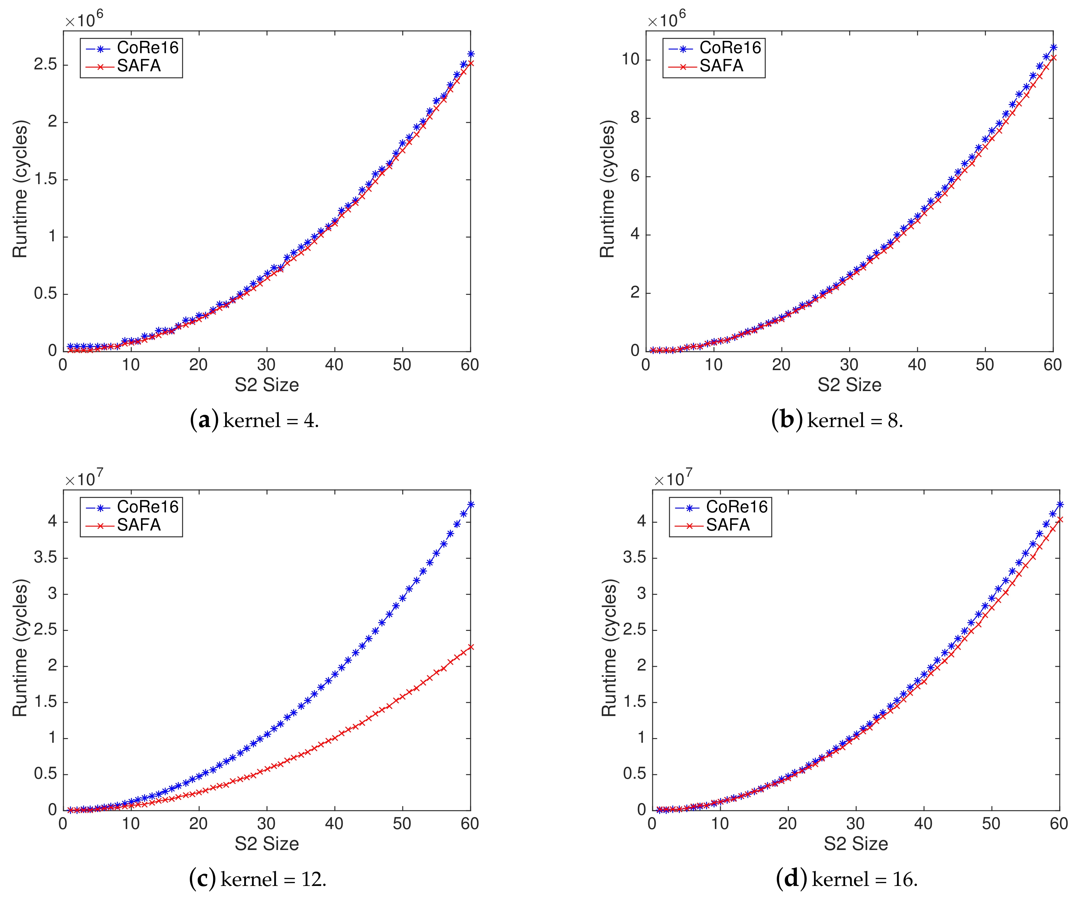
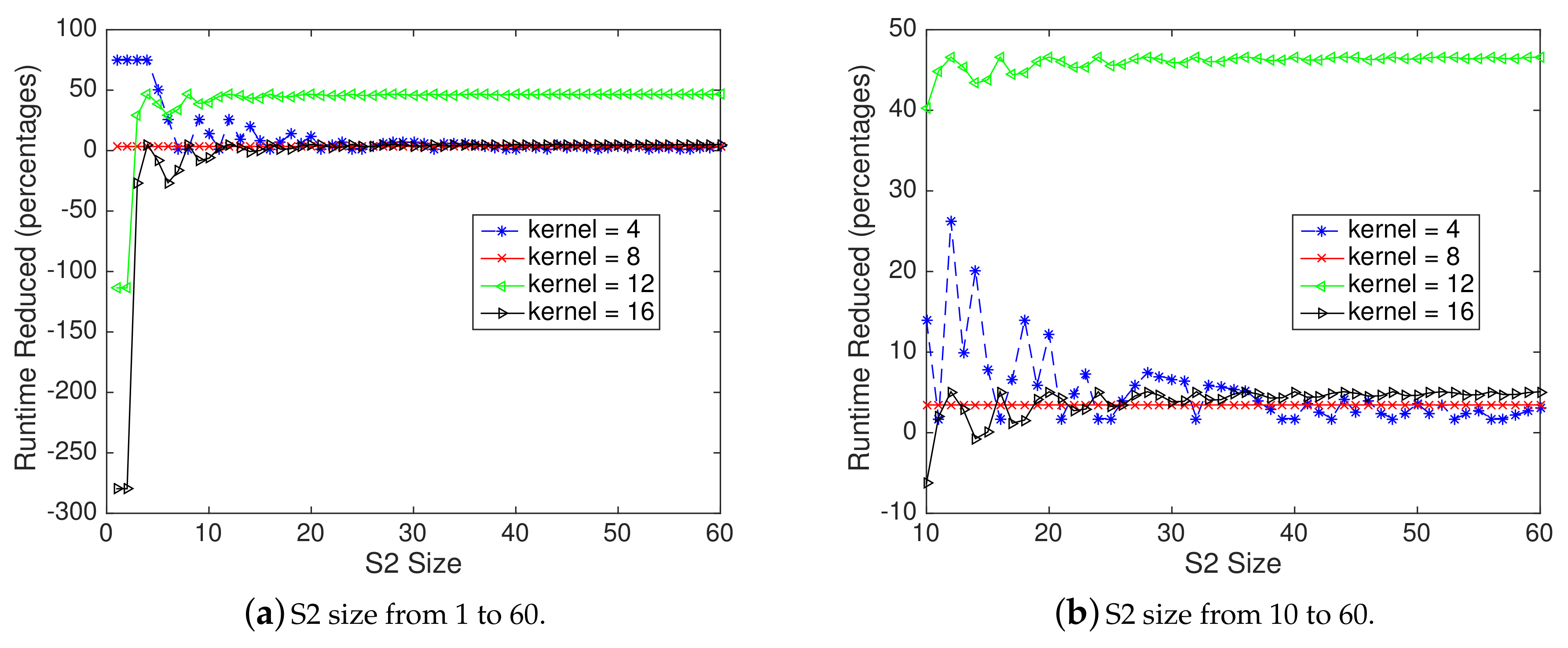
4.3. Comparison of Runtime

Figure 5 presents the effect of S2 size on runtime for different kernel sizes. As can be seen, the runtime of SAFA and CoRe16 increases with an exponential rate. When the S2 size is large, the HMAX model needs to calculate more pixels, resulting in a significant runtime increase.

Figure 6a reflects the percentage of SAFA runtime reduction compared to CoRe16. The horizontal axis S2 size varies from 1 to 60. We can see that in most cases, SAFA achieves better performance. Although SAFA’s acceleration effect is not as good as CoRe16 when kernel equals 12 or 16 and S2 size is small (less than 10), this only occupies a small proportion for the computation of HMAX model. To explain, CoRe16 uses the adder tree accumulation mechanism to calculate each pixel. When S2 size is small, its unit utilization is higher (see Section 4.5 for analysis).

Figure 6b shows the percentage of SAFA runtime reduction compared to CoRe16 when S2 size ranges from 10 to 60 (since most of the calculations are concentrated on it). As can be seen, SAFA performs better than CoRe16 under different kernel sizes. When kernel size ranges from 4 to 16, the average runtime is reduced by 11.18%, 3.44%, 39.67%, or 2.5%, respectively.

Note that we can acquire a significant speedup compared with CoRe16 when the kernel size is 12. The reason is that CoRe16 computes the larger kernels (8, 12, 16) output through the adder mechanism by the small one (4). CoRe16 mainly includes sixteen $4\times 4$ PE arrays with each used to accumulate the partial sums of the larger kernels. Thus, CoRe16 can process up to sixteen $4\times 4$ or four $8\times 8$ S2 kernels in parallel. It is also able to process one $12\times 12$ or $16\times 16$ kernel in parallel. When the kernel is 12, only twelve (equaling to kernel size, 75% of the whole array for CoRe16) $4\times 4$ PE arrays are utilized in CoRe16, and it does not work at full load. In contrast, SAFA produces output pixels in each PE and is able to perform at full load under different kernel sizes. For a fair comparison, we exclude the performance gain when kernel = 12 compared with CoRe16.

We can also see that a larger kernel for CoRe16 brings less runtime reduction. To explain, CoRe16 behaves more similarly to our SAFA with a larger kernel size. Specially, when the kernel is the largest (16), CoRe16 only produces an output pixel in one calculation, which performs like a more massive PE in SAFA. The average runtime is reduced by 5.7% under different kernel sizes except for kernel = 12 (since it is unsuitable for CoRe16).

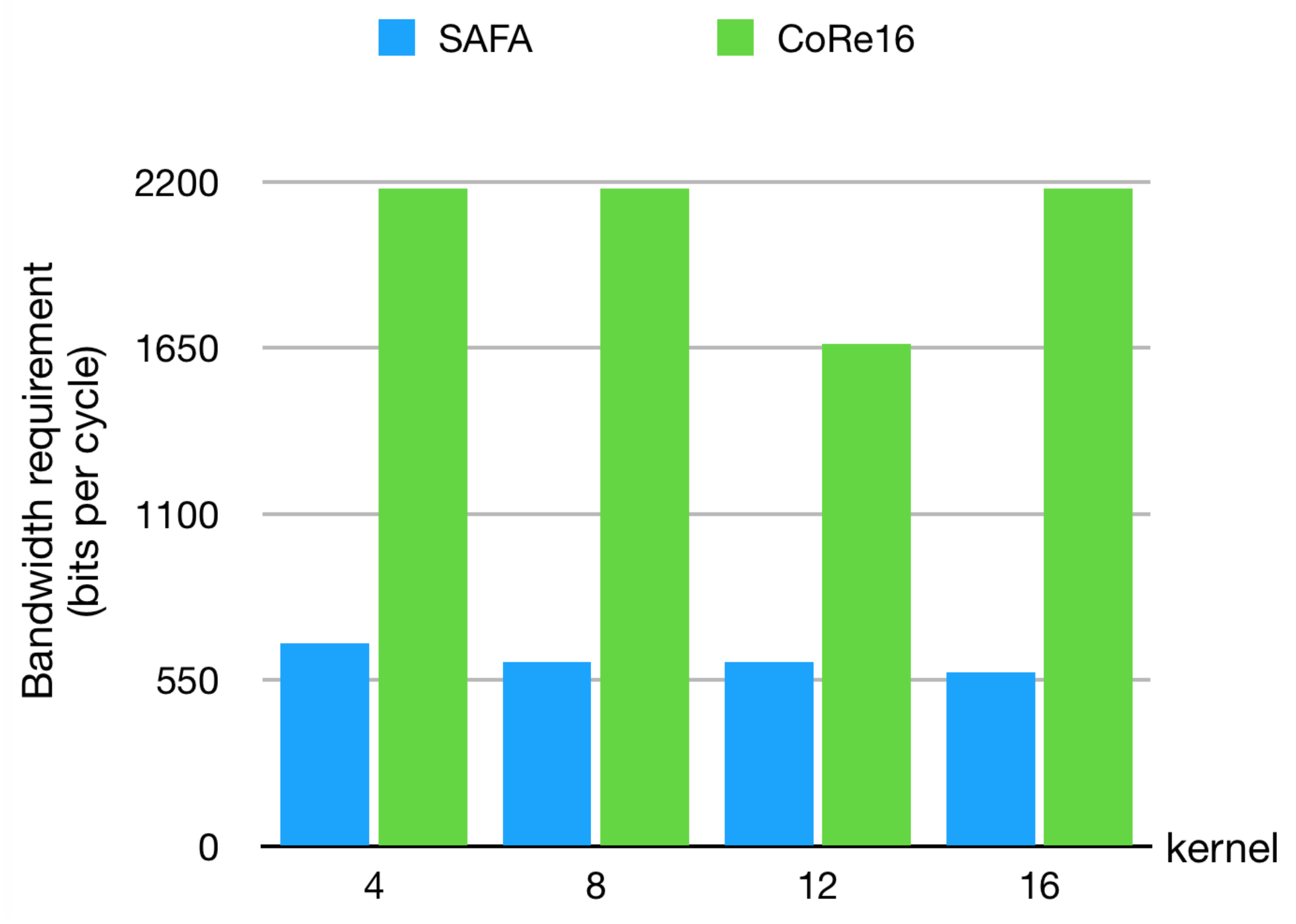
4.4. Comparison of Storage Bandwidth

Storage bandwidth is based on the maximum amount of data that the accelerator needs in a single cycle. Figure 7 illustrates the storage bandwidth requirement under different kernels. Note that SAFA needs less storage bandwidth compared with CoRe16 under different kernels. The reason is that SAFA transmits and reuses both input and patch data, while CoRe16, which merely reuses the patch group, needs a larger input data stream.

Meanwhile, as kernel size increases, the storage bandwidth required by SAFA gradually decreases and CoRe16 is almost unchanged except that the kernel size is 12. This is because, with the increase of kernel size, the single datum is multiplexed more times in SAFA at each cycle. CoRe16 calculates the output pixels of the larger kernels with the small one. In perfect combination matching (i.e., kernel size = 8 or 16), there is no change for the required bandwidth between them. The memory requirement reduction compared with CoRe16 is 3.24, 3.58, 2.74, or 3.78 times under kernel = 4, 8, 12, pr 16, respectively. Since when kernel size is 12, CoRe16 does not work at full load, the storage bandwidth of SAFA can be reduced by 3.53 times on average (except for kernel = 12) under different kernels.

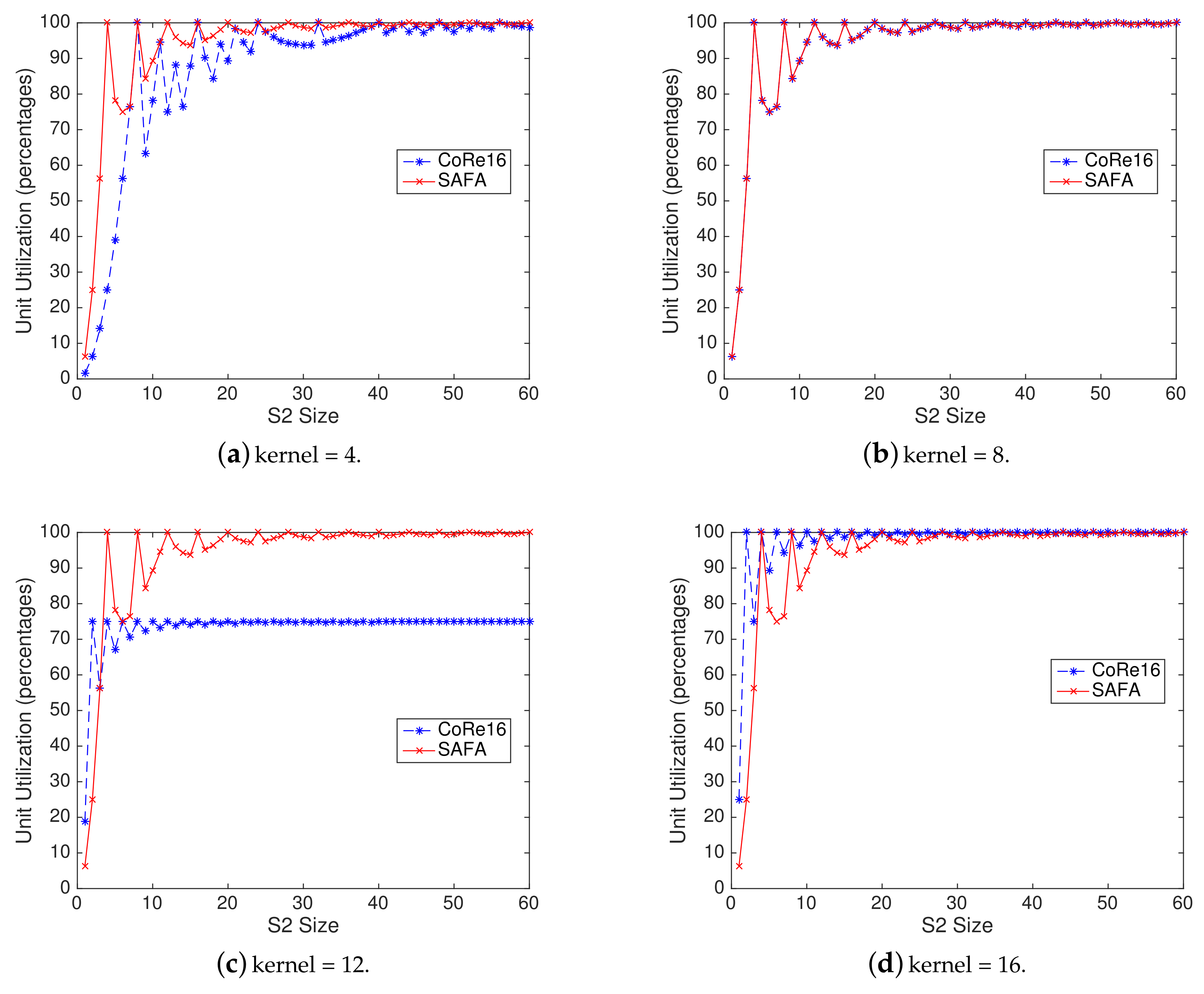
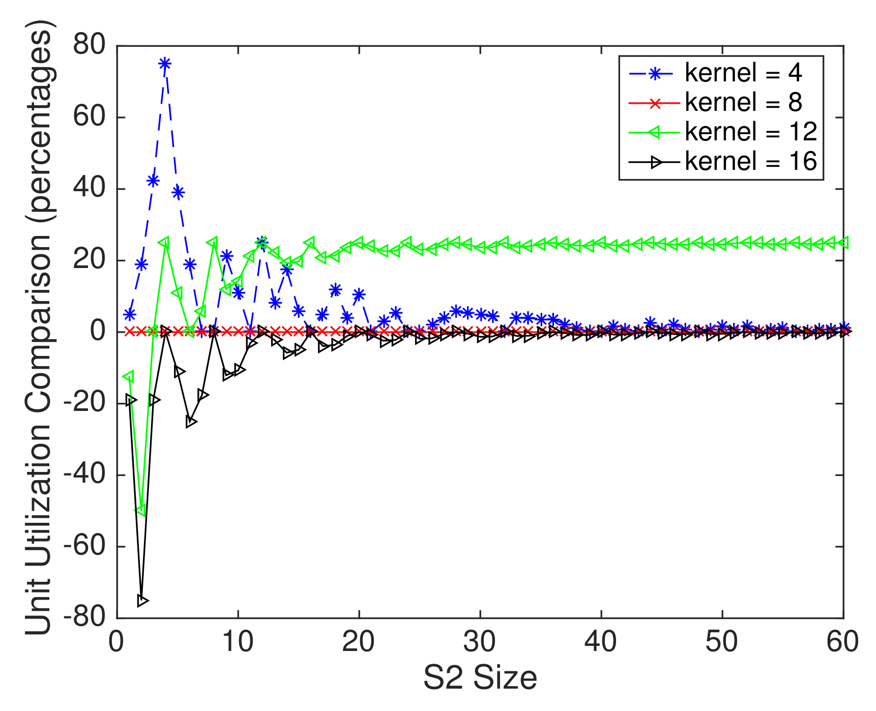
4.5. Comparison of Unit Utilization

Figure 8 presents the unit utilization for SAFA and CoRe16 under different kernels. We can see that SAFA performs well with a larger S2 size and reaches nearly 100% unit utilization under different kernels. The reason is that with the increase of S2 size, SAFA works more times at full load, resulting in fewer unused units. Under different kernels, SAFA unit utilization is constant. This is because SAFA calculates output pixels in each PE unit. The kernel size only influences the calculation time of output pixels in each PE unit.

For CoRe16, as S2 size increases, the unit utilization gradually becomes stable. Under different kernels, the unit utilization of CoRe16 is different. To explain, CoRe16 calculates output pixels by adder tree accumulation. With a larger kernel size, fewer pixels are calculated by CoRe16 when working at full load, and the utilization ratio is relatively higher.

To better reveal the unit utilization comparison between SAFA and CoRe16, Figure 9 shows the percentage of SAFA unit utilization improvement compared to CoRe16 under different kernels. We can see that in most cases (except for kernel = 12), SAFA unit utilization is close or better than CoRe16. When the kernel equals 12 or 16, and S2 is small (less than 10), SAFA unit utilization performs not as well as CoRe16. This is because CoRe16 only processes one output pixel for one patch group in that case, whereas SAFA produces sixteen output pixels for one patch group. When S2 size is small, SAFA is more likely not to perform at full load.

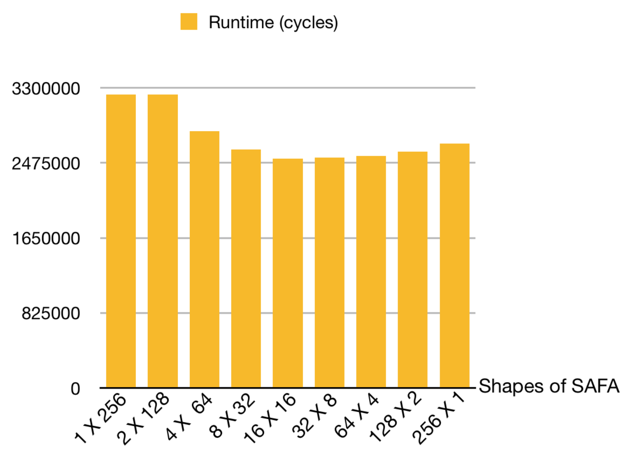
4.6. Sensitivity of Shape Array on Runtime

In this subsection, we still use Matlab to simulate the runtime of SAFA in different shapes realistically. Figure 10 presents the runtime of SAFA in different shapes. We can see that when the array size is $16\times 16$, the runtime is the shortest. This is because the square systolic array can make use of the patch group loop; i.e., the number of patch groups can be divided by 16. Meanwhile, the data loop can be utilized as well, and the unit utilization is high. Note that the closer the array is to a square, the shorter the runtime. Compared with $1\times 256$, $2\times 128$, $4\times 64$, and $8\times 32$, the runtime of SAFA is decreased by 21.9%, 21.8%, 10.7%, and 3.8%, separately. In comparison with $256\times 1$, $128\times 2$, $64\times 4$, and $32\times 8$, the runtime of squared SAFA is reduced by 6.2%, 3.0%, 1.3%, and 0.4%, respectively. Therefore, we choose a square array ($16\times 16$) for SAFA.

4.7. Area and Power Evaluation

The synthesis results on ASIC for SAFA and other reconfigurable accelerators are reported in

Table 2. Area and power evaluation for SAFA and other reconfigurable accelerators (28 nm). As can be seen, SAFA obtains the lowest power and area compared with the rest of the reconfigurable accelerators.

	Maashri et al. [14]	Park et al. [15]	CoRe16 [11]	SAFA
Area (${\mathrm{m}\mathrm{m}}^2$)	4.44	4.06	4.14	3.93
Power (mw)	3715.3	3390.1	3456.9	3320.8

. As shown in Table 2, SAFA is 3.32 W with 3.93 ${\mathrm{m}\mathrm{m}}^2$, which achieves the lowest power and area compared with the rest reconfigurable accelerators.

We also use frames per second (FPS) as a metric to indicate the processing speed for each PE in SAFA, CoRe16, and Park et al. [15]. Here, the image size is $256\times 256$, the same as CoRe16 [11].

Table 3. Area, power, and FPS evaluation for the PE in SAFA and other reconfigurable accelerators. The PE of SAFA also achieves higher FPS in contrast with other reconfigurable accelerators while maintaining lower power and area.

	Park et al. [15]	CoRe16 [11]	SAFA
Area (${\mathrm{m}\mathrm{m}}^2$)	0.0147	0.0154	0.0141
Power (mw)	12.6	13.1	12.2
FPS	1.74	1.69	1.81

presents the area, power, and FPS for the PE in S2 accelerators. We can see that our PE can obtain higher FPS compared with other reconfigurable accelerators while maintaining lower power and area. This is because, in SAFA, the input feature map and the patches can be reused to produce output pixels following the OS dataflow. This feature also helps to reduce the multiplexers utilized in the PE of SAFA, as most of the reconfigurable accelerators rely on multiplexers to select proper input pixels for further computation.

5. Conclusions and Future Work

In this paper, we proposed a systolic accelerator SAFA for HMAX-based multi-class object recognition algorithms. The core of SAFA was to calculate the corresponding output pixels in each PE using the OS dataflow. Meanwhile, our designed PE could avoid the overhead to accumulate partial sums in different PEs and lessen the multiplexers used in most reconfigurable accelerators. Data forwarding for the same input or patch parameters also reduced the required memory bandwidth. The results showed that SAFA reduced the runtime for the heaviest computing S2 phase in HMAX by 5.7%, and the memory bandwidth requirement was decreased by 3.53 × on average under different kernels (except for kernel = 12) compared with CoRe16. Besides, SAFA also provided lower power and area costs in contrast with reconfigurable accelerators from synthesis on ASIC. Future work is to optimize SAFA to support different computer vision algorithms, such as deep convolution neural networks.

References

1. Sanchez, J.; Soltani, N.; Chamarthi, R.; Sawant, A.; Tabkhi, H. A Novel 1D-Convolution Accelerator for Low-Power Real-time CNN processing on the Edge. In Proceedings of the IEEE High Performance Extreme Computing Conference (HPEC), Waltham, MA, USA, 25–27 September 2018; pp. 1–8. [Google Scholar]
2. Serre, T.; Oliva, A.; Poggio, T. A feedforward architecture accounts for rapid categorization. Proc. Natl. Acad. Sci. USA 2007, 104, 6424–6429. [Google Scholar] [CrossRef] [PubMed] [Green Version]
3. Liu, X.; Yan, M.; Bohg, J. MeteorNet: Deep learning on dynamic 3D point cloud sequences. In Proceedings of the International Conference on Computer Vision (CVPR), Seoul, Korea, 21 October 2019; pp. 9246–9255. [Google Scholar]
4. Iscen, A.; Tolias, G.; Avrithis, Y.; Chum, O. Label propagation for deep semi-supervised learning. In Proceedings of the Computer Vision and Pattern Recognition (CVPR), Long Beach, CA, USA, 13 June 2019; pp. 5070–5079. [Google Scholar]
5. Maximilian, R.; Tomaso, P. Hierarchical models of object recognition in cortex. Nat. Neurosci. 1999, 2, 1019–1025. [Google Scholar] [CrossRef]
6. Serre, T.; Wolf, L.; Bileschi, S.; Riesenhuber, M.; Poggio, T. Robust object recognition with cortex-like mechanisms. Trans. Pattern Anal. Mach. Intell. (TPAMI) 2007, 29, 411–426. [Google Scholar] [CrossRef] [PubMed]
7. Zhang, H.-Z.; Lu, Y.-F.; Kang, T.-K.; Lim, M.-T. B-HMAX: A fast binary biologically inspired model for object recognition. Neurocomputing 2016, 218, 242–250. [Google Scholar] [CrossRef]
8. Wang, Y.; Deng, L. Modeling object recognition in visual cortex using multiple firing k-means and non-negative sparse coding. Signal Process. 2016, 124, 198–209. [Google Scholar] [CrossRef]
9. Sufikarimi, H.; Mohammadi, K. Role of the Secondary Visual Cortex in HMAX Model for Object Recognition. Cogn. Syst. Res. 2020, 64, 15–28. [Google Scholar] [CrossRef]
10. Cherloo, M.N.; Shiri, M.; Daliri, M.R. An enhanced HMAX model in combination with SIFT algorithm for object recognition. Signal Image Video Process. 2020, 14, 425–433. [Google Scholar] [CrossRef]
11. Sabarad, J.; Kestur, S.; Park, M.S.; Dantara, D.; Narayanan, V.; Chen, Y.; Khosla, D. A reconfigurable accelerator for neuromorphic object recognition. In Proceedings of the Asia and South Pacific Design Automation Conference (ASP-DAC), Sydney, Australia, 9 January 2012; pp. 813–818. [Google Scholar]
12. Sufikarimi, H.; Mohammadi, K. Speed up biological inspired object recognition, HMAX. In Proceedings of the 2017 3rd Iranian Conference on Intelligent Systems and Signal Processing (ICSPIS), Shahrood, Iran, 6 December 2017; pp. 183–187. [Google Scholar]
13. Mutch, J.; Knoblich, U.; Poggio, T. CNS: A GPU-Based Framework for Simulating Cortically-Organized Networks; Massachusetts Institute of Technology: Cambridge, MA, USA, 2010. [Google Scholar]
14. Maashri, A.A.; DeBole, M.; Yu, C.L.; Narayanan, V.; Chakrabarti, C. A hardware architecture for accelerating neuromorphic vision algorithms. In Proceedings of the IEEE Workshop on Signal Processing Systems (SIPS), Beirut, Lebanon, 8 October 2011. [Google Scholar]
15. Park, M.; Kestur, S.; Sabarad, J.; Narayanan, V.; Irwin, M. An fpga accelerator for cortical object classification. In Proceedings of the Design Automation and Test Conference and Exhibition (DATE), Dresden, Germany, 19 March 2012. [Google Scholar]
16. Liu, B.; Chen, X.; Wang, Y.; Han, Y.; Li, J.; Xu, H.; Li, X. Addressing the issue of processing element under-utilization in general-purpose systolic deep learning accelerators. In Proceedings of the Asia and South Pacific Design Automation Conference (ASP-DAC), Tokyo, Japan, 20 January 2019; pp. 733–738. [Google Scholar]
17. Samajdar, A.; Zhu, Y.; Whatmough, P.; Mattina, M.; Krishna, T. Scale-sim: Systolic cnn accelerator simulator. arXiv 2018, arXiv:1811.02883. [Google Scholar]
18. Sze, V.; Chen, Y.H.; Yang, T.J.; Emer, J.S. Efficient processing of deep neural networks: A tutorial and survey. Proc. IEEE 2017, 105, 2295–2329. [Google Scholar] [CrossRef] [Green Version]
19. Poggio, T.; Bizzi, E. Generalization in Vision and Motor Control. Nature 2004, 431, 768–774. [Google Scholar] [CrossRef] [PubMed]
20. Liu, Z.; Dou, Y.; Jiang, J.; Wang, Q.; Chow, P. An FPGA-based processor for training convolutional neural networks. In Proceedings of the 2017 International Conference on Field Programmable Technology (ICFPT), Melbourne, VIC, Australia, 7 December 2017; pp. 207–210. [Google Scholar]
21. Riesenhuber, M.; Serre, T.R.; Bileschi, S.; Martin, J.G.; Rule, J. HMAX Tarball. Available online: https://maxlab.neuro.georgetown.edu/hmax.html (accessed on 26 February 2020).
22. Erik, L.M. Labeled Faces in the Wild: A Survey. Advances in Face Detection and Facial Image Analysis; Springer International Publishing: Basel, Switzerland, 2016. [Google Scholar]
23. Hwang, K.; Jotwani, N. Advanced Computer Architecture; McGraw-Hill Education: New York, NY, USA, 2016. [Google Scholar]
Figure 1. The HMAX model overview. The gray-value image is first processed by performing the convolution at four different orientations and eight scales (the full model uses 16 scales) through the S1 layer. The next C1 layer provides the local max (M) pooling over a neighborhood of the S1 layer in both scales and space. In the next stage, the S2 layer uses the GRBF unit with a set of patches which have been randomly sampled from a set of representative images [6]. At last, a global max pooling operation is provided over the S2 layer to generate C2 values.
Electronics 09 01690 g001
Figure 2. The structure of SAFA. SAFA is a 16 × 16 systolic array containing 256 identical and simple PEs. The key of SAFA is expressed as (1) local interconnecting and (2) shifting data transfer.
Electronics 09 01690 g002
Figure 3. Schematic diagram of a single PE in SAFA. Unlike the traditional systolic array where the PE performs MAC operation, our designed PE implements subtraction, multiplication, and accumulation operations to carry out the reduced GRBF function (details are illustrated in Section 2) in the S2 layer.
Electronics 09 01690 g003
Figure 4. The SAFA dataflow diagram. We mainly use the OS dataflow for SAFA. The green dashed line indicates the calculation sequence of each PE in SAFA. The same red color values A 1 , 4 represent the data reused in our dataflow. In contrast, the blue values donate the last pixels of the C1 input required to calculate an output pixel.
Electronics 09 01690 g004
Figure 5. Effects of S2 size on the runtimes of SAFA and CoRe16 under different kernel sizes. The runtimes of SAFA and CoRe16 increase with exponential rates.
Electronics 09 01690 g005
Figure 6. Percentage of SAFA runtime reduction compared to CoRe16. Note that when kernel size = 12, CoRe 16 does not work at full load due to the adder tree mechanism to produce an output pixel. For a fair comparison, we exclude the performance gain when kernel = 12 compared with CoRe16. However, we still achieve better performance. As shown in Figure 6b, the average runtime reduction compared with CoRe16 is 5.7% under different kernel sizes except for kernel =12 (since it is not suited for CoRe16).
Electronics 09 01690 g006
Figure 7. Storage bandwidth requirement for both SAFA and CoRe16. The storage bandwidth of SAFA is reduced by 3.53 times on average under different kernels (except for kernel = 12).
Electronics 09 01690 g007
Figure 8. Unit utilization comparison for SAFA and CoRe16. SAFA performs well with a larger S2 size and reaches nearly 100% unit utilization under different kernels. This is because SAFA works more times at full load with a lager S2 size, resulting in fewer unused units.
Electronics 09 01690 g008
Figure 9. Unit utilization improvement compared to CoRe16 under different kernels. In most cases (except for kernel = 12), SAFA unit utilization is close or better than CoRe16.
Electronics 09 01690 g009
Figure 10. Runtime of SAFA in different shapes. Note that a square array ( 16 × 16 ) for SAFA achieves the shortest runtime.
Electronics 09 01690 g010