Abstract
Due to the generation uncertainty of photovoltaic (PV) power generation, it has been posing great challenges and difficulties in maintaining the stability, security, and reliability of PV-storage systems (one kind of microgrid). To overcome these challenges and difficulties, this paper is concerned with secondary control and robust energy management for PVs in a grid-connected microgrid (MG) considering uncertainty. In our designs, to maintain the stable operation of PVs in MG, a novel secondary control method combining an event-triggered finite time sliding mode controller (FTSMC) and consensus controllers is proposed. Furthermore, a robust optimization framework is established to minimize the total cost of grid-connected MG involving the operation cost of multi-battery Energy Storage Systems (BESSes) and the electricity purchased from the main grid. To eliminate the effects of PV uncertainty, the optimization problem with uncertain constraints is converted into a new optimization problem with only deterministic constraints by using the box theory to represent the PV outputs. In other words, the robust optimization strategy makes uncertain boundaries easier to be represented by setting all uncertain parameters into an uncertain domain involving all typical extreme cases. Then, a particle swarm optimization (PSO) method is employed to solve the newly converted optimization problem. Finally, the experimental results validate the effectiveness of the proposed integrated framework.
1. Introduction
Due to growing shortages of fossil energy and environmental deterioration caused by fossil energy, lots of countries in the world are committed to the research of renewable energy, and their high attention and strong support from relevant policies have significantly promoted the rapid development of photovoltaic (PV)-storage system. And in fact, this system is one kind of microgrids (MGs) (i.e., it is a small power grid that includes distributed generators (DGs), loads, and battery energy storage systems (BESSes)). As a result, PV power generation has become an important power source in the world. For the PVs, we must first make sure that they can maintain stable operation in MG. Therefore, the design of a reasonable controller is the first problem to be solved in this study. In addition, PV power generation incorporated into MG include uncertainty and volatility of the PV output, and in practice, it is difficult to predict such uncertainty and volatility. Thus, it always causes great challenges and difficulties for MGs in implementing reliable operation, ensuring power quality, achieving energy management, and maintaining economic efficiency [1,2]. Notably, in the presence of uncertainty, the traditional deterministic optimization algorithm may not be applicable since there is a deviation between the predicted values of PV generation and actual values of PV power generation [3]. Therefore, the second problem we need to solve is how to effectively complete the reasonable scheduling problem when considering the uncertainty of PV.
The control of MG can be divided into the following three kinds of method: 1. Voltage control; 2. Frequency control; 3. The power control. Among them, the control of voltage and frequency is the precondition of stable operation of MG. If the MG operates in the grid-connected mode, the output voltage and frequency of each DG in the MG are affected by the main grid, and their voltages and frequency will be consistent with those of the main grid. Therefore, in general, we only need to consider how to design an appropriate control strategy to maintain the stable operation of MG when the grid-connected MG is off grid (i.e., it is switched in the islanded mode). Now, there are also some related methods proposed, which can be roughly divided into centralized, decentralized, and distributed. Among them, the most promising method is the distributed control method. This is because the distributed method can not only overcome the shortcomings of single point fault in the centralized method, but also overcome the problem of control asynchrony in the decentralized method. At present, the use of the distributed method usually needs communication network. The related literatures are as [4,5,6,7,8,9]. In these studies, a reasonable power sharing was completed in [4] by adding virtual impedance in MG. A consensus-based control method was proposed in [5]. Through this method, the average voltage and current data was used to realize the power sharing and voltage restoration. Another distributed strategy was proposed to accomplish reactive power sharing in [6]. Based on the voltage and current data of DGs, there was a distributed control method proposed in [7] to achieve power sharing. However, no disturbance problems were considered in [4,5,6,7]. In addition to the above three kinds of control strategies, there is also a kind of control which is in the process of development, that is, event-driven control. For example, a self-triggered communication enabled control was designed in [8]. Another event-based distributed active power sharing control was proposed in [9]. This kind of method can save communication cost. However, the above literature does not consider how to improve the convergence rate and anti-disturbance ability at the same time. Thus, it is likely that even if the disturbance is successfully suppressed by designing the corresponding observers and controllers, the required time for completing control is too long, which is not conducive to use in practice.
In addition to the control methods, in recent years, there have been considerable research results in existing literature regarding the optimization issues for power systems such as MG [10]. A kind of robust energy management strategy based on fuzzy prediction is proposed in [11], i.e., the data obtained from fuzzy prediction is used to complete the energy management. A robust optimization management strategy considering price uncertainty and demand side response was proposed in [12]. In [13], a demand-based robust energy management strategy was proposed for the MG with a high proportion of renewable energy penetration. Another demand-based robust strategy was proposed in [14] to complete the day ahead scheduling. The robust optimal management strategies considering various uncertainties were designed in [15,16]. Aiming at the energy management problem of MG cluster, a robust scheduling strategy considering various uncertainties was proposed in [17]. In [18] and [19], the corresponding robust energy management strategies were proposed for the possible multi-period attacks and natural disasters in MG. It can be seen from the analysis of literature [11,12,13,14,15,16,17,18,19] that the problem to be solved in robust optimization is the uncertainty in energy management. In fact, the BESS can effectively solve the problem of uncertainty and volatility for PV power generation output. When PV power generation is greater than the load, the BESS can be charged, whereas it can be discharged in the case that PV power generation is less than the load. By coordinating the BESSs, the accommodation capability of serving PV power can be significantly improved [20,21]. Zhang et al proposed a differential evolution with sequential quadratic programming in [22] to optimize the wind power optimization model under different uncertainty levels. In addition, wind power uncertainty can be properly handled by robust optimization methods with different levels. Therefore, it is of importance and significance for MGs to develop a new optimization framework by taking into account the characteristics of BESSs in the presence of PV uncertainty, which motivates our current study.
In summary, previous distributed control and optimization frameworks have their own problems. To effectively solve the problems mentioned above, we have done the following work in this study (i.e., the innovations).
(1) In view of the situation after the grid-connected MG is off the main grid, a novel secondary control method combining event-triggered FTSMC and consistency controllers is designed to maintain the stable outputs of PVs. By using the FTSMC, we can effectively suppress the disturbance data. Meanwhile, the suppression work can be completed in the finite time. By using the event-triggered mechanism, the two SMCs can be effectively combined.
(2) A robust optimization scheduling model for grid-connected MG with high proportion PV is established. It can ensure the strong robustness caused by the uncertainty of PV generation output.
(3) Comparing with the papers above without considering BESS to suppress the uncertainty and volatility, this paper presents the model including multi-BESSs, fully considering physical constraints of BESS.
The integration designs in this study are shown in Figure 1, and it can be seen that we have to design two parts, namely the secondary control strategy and robust optimal management strategy. The secondary controller includes the event-triggered mechanism, FTSMC, and consistency controller. For energy management strategy, it includes multi-objectives and robust constraints. See the following sections for the designs of the above parts. The research process of this paper is combined in the following order. The design details of the control strategy are introduced in Section 2. Section 3 focuses on the problem formulation of the grid-connected MG. Section 4 describes the formulation of a robust optimization model of MG. Meanwhile, this Section also expresses the particle swarm optimization which is used to solve the model. The case study consequences are described in Section 5. Finally, Section 6 summarizes the study and presents the conclusions.
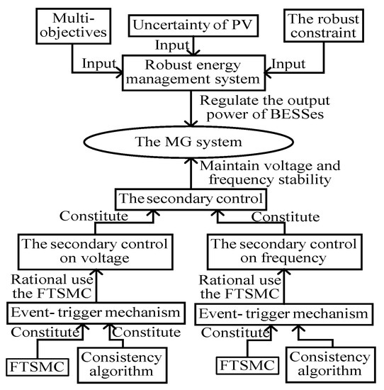
Figure 1.
The integrated design of control and energy management.
2. Design of the Secondary Control Strategy
For grid-connected MG, the working mode of each DG (e.g., PV and BESS) is P/Q mode. Therefore, the output voltage and frequency of each DG are affected by the main grid. In other words, its voltage and frequency are generally stable. However, once the MG is disconnected from the main grid, we need to design appropriate methods to maintain the voltage and frequency stability. To solve this problem, we have designed the following secondary control strategy. The corresponding control structure is as the Figure 2.
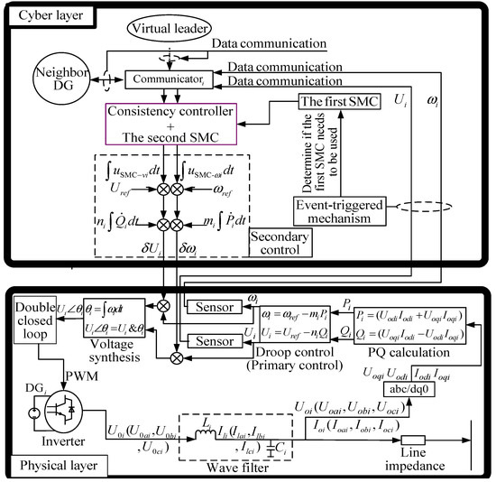
Figure 2.
The designed control structure.
2.1. Design the Consensus-Based Secondary Controller
In the past, the output voltage and frequency of DG were regulated by droop control. However, the droop control is obtained by approximating the generator operation. Therefore, this control method will cause errors between the controlled variables and the reference values. To solve this problem, it is necessary to apply secondary control to DG. In this study, the designed secondary control method needs the consensus algorithm to complete. And the advantage of this algorithm is to complete the synchronous control of DGs. Moreover, this algorithm can avoid single point chain failure. Moreover, due to the existence of a virtual leader, this algorithm can directly set the state of virtual leader to achieve the stable output of voltage and frequency. To better explain the design process of secondary control, the following basic theory is presented.
2.1.1. The Related Basic Theory
Graph theory: Each DG in a MG can be observed as a node, and these nodes constitute a directed graph. In this graph, if the data of the jth node can be transmitted to the ith node, then we call the is positive, where represents the relationship between the jth DG and the ith DG. Further, if cannot be transmitted from the jth DG to the ith DG, then there should be [23].
Consistency algorithm: For a directed graph, if the controller as is established for the ith node, then these controlled variables of nodes will be adjusted to . Among them, are the data of the virtual leader and represents the relationship between the ith DG and the virtual leader. If the ith DG can receive a message from the virtual leader, then is positive. Otherwise, is negative [24].
2.1.2. Design of the Secondary Controllers
Voltage and frequency secondary control are based on the droop controller. In this study, the completion process of the secondary control is as follows: First, based on the output voltage, frequency, and consistency algorithm, the feedback on voltage and frequency will be generated. Second, the feedback will be added to the output of the droop control to make up for these shortcomings of droop control. The specific controller is as follows.
Based on the previous designs, this subsection is used to design the secondary controller to improve the control effect on DERs when communicator interruption occurs in MG. To better explain these designs, for the ith DER, the droop control equation can be described as
where and are the droop coefficients; and are the reference values of frequency and voltage, respectively; and are the active and reactive power, respectively. Furthermore, the goal of secondary control on voltage is to adjust to . From Equation (1), the following equation can be established.
where is an auxiliary variable. Based on Section 4.1 and Section 4.2, the secondary controller on voltage can be designed as
where and are the output voltage of the ith and the jth DERs, respectively; is the voltage of virtual leader. It is constant and known; and are all gains in the controller.
Similar to the secondary control on voltage, the secondary control on frequency can be designed in the same way. Based on Equation (1), the following differential equation can be obtained.
where is also an auxiliary variable. Similar to the process of designing a secondary controller on voltage, the secondary controller on frequency can be designed as
where and represent the frequency of the ith and jth DERs respectively; is the frequency of virtual leader; and are gains.
2.2. Analyze the Influence of the Disturbance on the DG
When the MG changes from grid-connected mode to islanded mode, the DG usually operates in the droop control mode. In this switching process, external disturbances are likely to occur in the control process. Therefore, it needs to further suppress the influence of external disturbance on the stability of MG. To solve this problem, an event-triggered FTSMC-consistency algorithm is proposed. The specific analysis of the influence of the external disaturbance o DG is as follows:
To better analyze the influence of the designed secondary controller on the stability of the DG, the cyber layer and the physical layer should be combined to construct the following small signal model. The corresponding analysis is as below: For the ith DG in a MG, the output active and reactive power of this DG are
where and are output active and reactive power of the ith DG; is the voltage of the electric node; is the angle of the voltage; is the angle of the line impedance; is the injected voltage of the ith DG; and are the active and reactive powers of load.
Through filtering, the power will be transformed into
where is the parameter of the filter. If we assume there are small disturbances ΔUi and Δφi in the ith DG, the influences on power can be described as
where ; ; ; . If the influence of the cyber layer on the physical layer is considered by us, there will be
Based on Equation (10), Equation (11) can be obtained.
And the analysis above can be described into a figure as Figure 3.
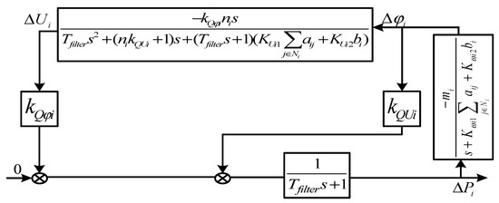
Figure 3.
The small signal model of the ith DG.
As illustrated in Figure 3, it was found that the small signal model is a closed-loop system. Therefore, if the related parameters are not selected properly, the system will not be able to maintain stable operation.
2.3. Design of the FTSMC-Consistency Controller
In this design, the FTSMC is used to suppress the disturbance. Further, the SMC can complete the suppression work in the finite time. The corresponding design process is as follows.
2.3.1. Design of the FTSMC
In the cyber layer, there is communication data disturbance in the process of transferring data from the physical layer to the cyber layer. It requires designing the appropriate method to solve the problem.
For the convenience of explanation, we take a MG with two DGs as an example to explain the design process of the secondary controller. Under this condition, the designed consensus controllers considering data disturbance are as below:
where , , , and are gains in the consistency controller; and are the disturbance data ; . Then, Equations (13) and (14) can be obtained.
From Equation (14), it can be found that the controlled system needs to be decoupled. In this paper, the feedback matrix is used to decouple the system (the dashed part). The specific method is as follows.
Equation (14) can be also written as below:
Meanwhile, the feedback matrix is set as . After adding the feedback matrix, Equation (14) is changed as below:
The selection rules of are as below:
where and are used to design the SMC. Further, the specific process is as the follows. At first, the sliding model surface is designed as below:
where and are the coefficients of the sliding mode surface. Then, we choose to design the SMC as , and there will be
After setting and , there will be
Afterward, we take the Lyapunov function as , and its derivation is
Finally, we set in Equation (20). Thus, because we want to make the equation satisfy Lyapunov stability, there should be
where is the switching gain in the protocol, and .
2.3.2. Design of the Event-Triggered Mechanism
For the event-triggered mechanism, the main function is to determine whether to use the FTSMC. This is because the application of SMC will cause catting in the MG, which will affect the stable operation. Moreover, with respect to MG, its voltage and frequency have corresponding application range. As long as the disturbance does not cause the overshooting of the MG to exceed its allowable range, we can only use the consistency algorithm to complete the secondary control. For the specific design of the triggered mechanism, please refer to reference [25]. The trigger events can be defined as overshoot and steady-state error caused by disturbance data. The trigger process is as below: 1. When the external disturbance makes the overshoot in the secondary control exceed the allowable range, SMC will be used directly to suppress the disturbance; 2. When the overshoot in the secondary control process caused by external disturbance does not exceed the maximum allowable range, it is necessary to judge whether the steady-state error caused by the disturbance will exceed the allowable range; 3. When the steady-state error does not exceed the allowable range, we do not use the FTSMC to suppress the disturbance; 4. Otherwise, we still need to use SMC to suppress the disturbance first. For the calculation methods of overshoot and steady-state error, see the literature [25].
2.4. Design the Event-Triggered Secondary Controller
Based on the designs in the Section 2.1, Section 2.2 and Section 2.3, the event-triggered mechanism can be added to regulate the voltage and frequency. The improved secondary controllers for the ith DG are as follows:
3. Design of the Robust Energy Management Strategy
The designed structure of energy management strategy is illustrated in Figure 4.
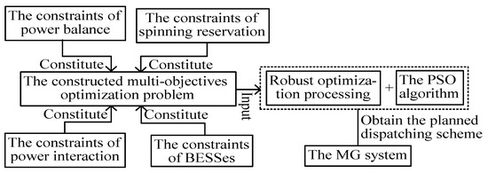
Figure 4.
The simplified energy management system.
3.1. Model of PV Power Generation
The principle of PV power generation is to covert solar energy directly into electrical energy. The power output of a PV module is usually adjusted into the standard test conditions, where the solar radiation intensity reaches 1000W/m2 and the battery output is 25 °C, which can be described as follows [17]:
where is the actual output of PV output at time ; is the actual radiation intensity at time ; STC means the standard test condition where is the solar radiation intensity; is the rated output of PV; is the temperature; is the temperature coefficient of power; is the temperature of battery at time .
It is commonly known that the random distribution of PV outputs is difficult to obtain while the basic interval of PV outputs can be measured easily. Thus, such uncertainty constraints of PV should be carefully taken into account for achieving optimization objectives. Here, we describe the uncertainty of PV output as a box constraint, which can be expressed as follows:
where is the actual output of PV at time ; is the predicted output of PV at time ; is the output fluctuations of PV at time ; is the dispatch interval coefficient of PV at time and . When , the predicted value of PV is equal to the actual value, implying the system has poor robustness because the influences of uncertainty in prediction are not considered. It is clear to see that, with the increase of , the robustness of the system can be improved, whereas the economy of the system will be reduced. and are the maximum and minimum output fluctuations of PV at time , respectively.
3.2. Optimization Objective
Since the cost of PV power generation is mostly zero, it can be ignored in our optimization formulation. As a result, the total cost of a grid-connected MG amounts to the operation cost of multi-BESSes and the electricity purchased from the main grid, which can be expressed as follows:
where is the total cost of grid-connected MGs; is the total time period; is the quantity of BESS; is the charging/discharging cost of BESS; is the power of BESS at time ; is the power interacting with the main grid at time . When , is the TOU price for purchasing power; when , is the TOU price for selling power.
3.3. Constraints
When devising an optimization scheme for a MG, it is essential and necessary to ensure that various physical constraints can be completely satisfied. In this paper, we consider the following physical and operational constraints:
(1) Power balance constraint
(2) BESS constraint
where is the capacity of BESS at time . is the time interval, and are the discharging and charging power of BESS at time , respectively. When , the BESS is discharging at time , otherwise means the BESS is charging at time . and are the maximum discharging and charging power of BESS, respectively. and are the maximum and minimum capacity of the BESS, respectively. is the rated capacity of the BESS.
(3) Power interaction constraint
where and are the maximum power that can be purchased from the main grid and the maximum power that can be sold to the main grid, respectively, and .
(4) Spinning reservation constraint
where is a coefficient for the spinning reservation rate required by MGs at time , and .
In summary, the optimal energy management of connected-grid MGs can be achieved by addressing the following optimization issue.
4. Robust Optimization Framework
4.1. Design of the Robust Optimization Problem
It is noted that the output of PV (i.e., the Equation (24)) includes uncertainty, which can be converted into a box constraint. As a result, in the presence of such uncertainty, it becomes very difficult to achieve the optimization issue (i.e., Equation (26)) with the physical constraints as Equations (27)–(34). To overcome this difficulty, we first need to eliminate the influence of uncertain PV output.
Substituting the power balance constraint as Equation (27) into the spinning reserve constraint as Equation (34), one can get:
Substituting Equation (30) into Equation (36), one obtains
Due to the dual theory, it is easy to know that:
Then, relaxing the constraint limits of PV power output, we define a Lagrange function as:
where are the Lagrange multipliers. Taking the partial derivative of Equation (39) with respect to yields
Then, it is clear to see that
Based on the analysis above, the optimization issue with the uncertainty of PV output can be equivalently transformed into:
Notice that Equation (42) provides a new robust optimization framework in which the uncertainty of PV output is no longer involved.
4.2. Particle Swarm Optimization
It is well known that a PSO algorithm has several advantages of being simple in structure, easy to implement and efficient in searching for global and individual optimum values and refreshing their positions. Moreover, the PSO algorithm shows good ability of searching. The PSO algorithms first initialize a group of particles randomly, then seek the solution space according to the fitness value, and find the optimal solution by the iteration of the given velocity and position updates. Therefore, a PSO algorithm is employed to address the optimization issue as Equation (42). The updates of velocity and position update are given as follow:
where is the number of current iteration; and are the learning factors, indicating the ability of particles to self-summarize and learn from groups; and are the random numbers between 0 and 1; is the position of the particles in the iteration; is the velocity of the particles in the iteration; is the optimal position of the particles in the current optimization process; is the optimal position of the particle population in the current optimization process.
Now, so as to solving the optimization issue as Equation (42), the PSO algorithm is given as follows
Step 1. Initialize the position and velocity of particles according to the constraints in the model;
Step 2. Set the fitness function according to the objective function, and calculate the fitness value of the current particle;
Step 3. Update and according to the calculated fitness value;
Step 4. Update the particle velocity and position according to Equations (43) and (44), respectively;
Step 5. If the number of iterations exceeds the constraint or the loop condition is satisfied, terminate the update. Otherwise, return to Step 2.
5. Experimental Results
In this paper, so as to verify the effectiveness of the proposed method, an MG mode is constructed as in Figure 5. In this experimental model (see the specific Simulink model in the Appendix A), the constituted parts are as below: four PVs, three BESSs, one fixed load, line impedance, one shiftible load, the communication network and the secondary control system etc. Further, in this model, the communication network among these DGs and BESSs is used to simulate the control effect of secondary control. To verify the effect of the energy management strategy, we simulate the planned output of BESS and main-grid based on the predicted output power of PVs. For this experiment, the used MG model for experiments is also as the Figure 5. The related experimental data is as shown in the Table 8, and the load demand is time-varying. The reason for using the data in this table is because we want to make the experimental process closer to the actual power consumption situation. However, different MG systems can be also used to verify the effectiveness of the proposed methods. The reasons for this are as below:
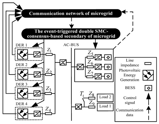
Figure 5.
The related MG model in experiments.
For secondary control strategies: The contributed strategies have combined sliding mode control and consistency control. For different controlled systems, the difference that may be brought to the secondary control is the difference in communication topology. However, this does not affect the effect of the secondary control. In other words, the secondary control can always adjust the output voltage and frequency of DGs to their respective reference values.
For the robust energy management strategy, the differences brought by different experimental models are reflected in the objective function and constraints. The reason for this is that the different experimental systems may have different physical typologies. However, we can still use the contributed strategy to solve the uncertainty problem of PV generation. Furthermore, we can still use the PSO algorithm to complete the scheduling task by solving the multi-objective optimization problem.
In summary, the MG model in Figure 5 is still used as the experiment object for Experiments 1 and 2. However, there is also a difference in that only load 2 is considered in the Experiment 2. In this way, the load demand varies across different time periods. This can also make the experimental results more objective. In conclusion, the MG model used in Experiments 1 and 2 are different.
Remark 1.
In Figure 5, the fixed load refers to the constant power load and it is usually the critical load, such as refrigerators used in homes or vending machines on the street. The characteristic of this type of load is that the power supply system should give priority to ensuring the normal use of this type of load. In addition, the electricity consumption of this type of load for each hour of the day is basically unchanged. Moreover, loads 1 and 2 mentioned are all constructed by a single load. The difference is that the load 1 is a constant power load, and it corresponds to the main load in the constructed MG system. Meanwhile, load 2 is time-varying, and it can be seen as a shiftible load (e.g., the washing machine) in the MG system. This kind of load can be used in different time periods according to the actual needs. Therefore, its power consumption in different time periods is also different.
To carry out Experiment 1, we mainly build the MG model and communication network based on the Simpower systems in Matlab/Simulink 2013a. Also in the platform of MATLAB/Simulink 2013a, so as to carry out the Experiment 2, we build programs corresponding to the objective function, constraints, and PSO algorithm to complete the dispatching task.
Remark 2.
The communication data and the control signal will be transmitted by different channels. The communication data were obtained by the PVs or BESSs in the physical system through droop control. In addition, these data will be input into the consistency controller to generate the corresponding regulation. The control signal is generated by the consistency controller in the communication network. Its main function is to complete the adjustment (i.e., the secondary control) of output voltage and frequency of PVs and BESSs.
In summary, the most obvious difference here is that the communication data are mainly used in the communication network, and the control signal is mainly used in the physical system.
In these experiments, the related experimental parameters are shown in Table 1.

Table 1.
The used parameters in experiments.
The related communication topology is shown in Figure 6. The experimental process and results are presented in the following subsections.
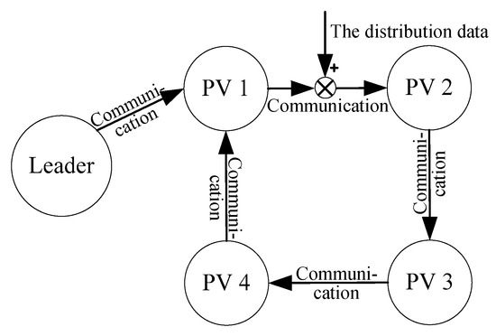
Figure 6.
The related communication topology of PVs.
The explanation of Figure 6 is as below: For the proposed secondary control strategy, all the methods used are based on consistency control. To achieve the corresponding control tasks, the corresponding communication network of the controlled system should be constructed as a directed connected graph. In other words, the communication network should contain a directed spanning tree, and the leader should be the root node in the tree. For this reason, the used communication network is built as the Figure 6. In this network, the directed tree (i.e., the connection relationship) is as follows: leader-PV 1-PV 2-PV 3-PV 4-PV 1. To further verify the effectiveness of the proposed SMC, we artificially add disturbance data to the controlled system, and then verify whether it can be suppressed by using SMC. Thus, we can verify that whether the normal progress of the consistency control can be maintained. More specifically, we have added step signals to the data (including voltage and frequency) transmitted from PV 1 to PV 2 to act as disturbance signals which may occur in the communication process. For example, if the step signal and are added to voltage signal and frequency signal , the two signals will be changed to and .
For the communication network in Figure 6, the related communication channels in a real MG between two nodes can be constructed through WiFi. However, in this article, the communication channel is constructed by the channels module of the communications system toolbox in Matlab/Simulink 2013a. This is because, in such an experimental environment, the communication disturbance can be better simulated.
5.1. Experiment 1: Verify the Control Effect on Secondary Control
In this section, the main experiments can be divided into four parts: 1. Verify the effect of the proposed secondary controller without considering the line impedance of BESSs and loads; 2. Verify the effect of the event-triggered mechanism; 3. Verify the effect of the proposed secondary controller considering the line impedance of BESSs and loads; 4. Verify the effect of the proposed secondary controller when the load is changed in different time periods. The communication data and control signals involved in the secondary control are summarized in the Table 2.
Table 2.
The involved communication data and control signal in the secondary control progress.
The specific experimental results are shown in the Section 5.1.1, Section 5.1.2, Section 5.1.3 and Section 5.1.4.
5.1.1. Case 1: Verify the Effect of the Secondary Controller without Considering the Line Impedance of BESSs and Loads
In this case, only the four PVs are used as the experimental objective to carry out the related experiments. To verify the control effect of the secondary controller and the SMC, we have carried out experiments in three situations. The specific experimental process is illustrated in Table 3.
Table 3.
The operation process in Case 1.
The experiment results are illustrated in Figure 7.
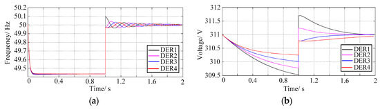
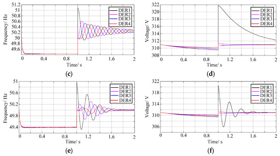
Figure 7.
The control effect of the SMC. (a) The control effect on the frequency under the situation 1; (b) The control effect on the voltage under the situation 1; (c) The control effect on the frequency under the situation 2; (d) The control effect on the voltage under the situation 2; (e) The control effect on the frequency under the situation 3; (f) The control effect on the voltage under the situation 3.
In Figure 7a,b, we can see that the droop control will obviously cause the controlled voltage and frequency to deviate from the desired reference values. Under normal communication condition, the secondary control will restore the output voltage and frequency of each DG to 311 V and 50 Hz before t = 2s. Moreover, during the regulation of secondary control, the output voltage and frequency of each DG will always be limited within the allowable range. From Figure 7c,d, we can find that because of the external disturbance in communication data, the effect of secondary control will be affected. In this case, the output voltage and power of each DG cannot be restored to the reference value within 1 s. It can be seen that the disturbance will not only affect the convergence effect of the secondary control, but also affect the convergence speed. In Figure 7e,f, we can find that the external disturbance data will be suppressed to zero. In the process of consistency control, we can still restore the output voltage and frequency to the reference value before t = 2 s. In other words, the proposed FTSMC can suppress the disturbance data effectively.
5.1.2. Case 2: Verify the Effect of Event-Triggered Mechanism
To verify the effect of event-triggered mechanism, we take the disturbance data in the data transmitted by PV 1 as an example to carry out simulation experiments. To verify the effect of the event-trigger mechanism from different situations, there are three kinds of situation carried out. See the specific experimental situations in the Table 4.
Table 4.
The operation process in Case 2.
The experiment results are as the Figure 8.
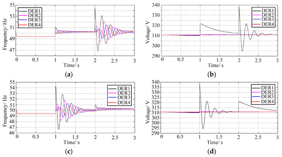
Figure 8.
The effectiveness of the event-triggered mechanism; (a) the variations of voltage in Experiment 1; (b) the variations of frequency in the experiment 1; (c) the variations of voltage in Experiment 2. (d) the variations of frequency in Experiment 2.
The corresponding analysis is as below: From the Figure 8a,b, we can see that the trigger mechanism will not be triggered after t = 1 s because the overshoot caused by the disturbance data will not exceed the maximum range allowed by MG. Therefore, we will still use only the secondary controller to adjust the output voltage and frequency of each DG. When t = 2 s, the trigger event will be triggered because the overshoot caused by the disturbance is 30 V and 5Hz respectively. In other words, FTSMC will be used to suppress external disturbance. Based on Figure 8c,d, we can find that the variations of voltage and frequency are opposite to Figure 8a,b. Moreover, under the control of the event-triggered mechanism, the controlled voltage and frequency of each DG will be eventually adjusted to their respective reference values.
5.1.3. Case 3: Verify the Effect of the Proposed Secondary Controller Considering the Line Impedance of BESSs and Loads
In the experiment to verify the effect of the secondary controller without considering the line impendance of the BESSs and loads, we only take four parallel PVs as an example. However, in practice, we also build a similar communication network for BESS. This is because BESS also relies on the droop control of the inverter to supply power for loads. In addition, BESS and loads have corresponding line impedance. When considering that line impedance exists in MG, it is necessary to verify whether the proposed secondary control strategy is still effective. In this case, the related communication topology of BESSs is shown in Figure 9. The related parameters of the BESSs and loads shown in Table 5, while the related control process is as in Table 6, and the experiment results are shown in Figure 10.
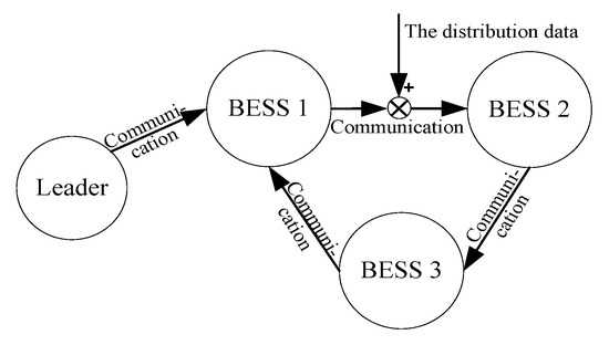
Figure 9.
The related communication topology of the MG.
Table 5.
The related parameters of the BESSs loads.
Table 6.
The control process of BESSs.
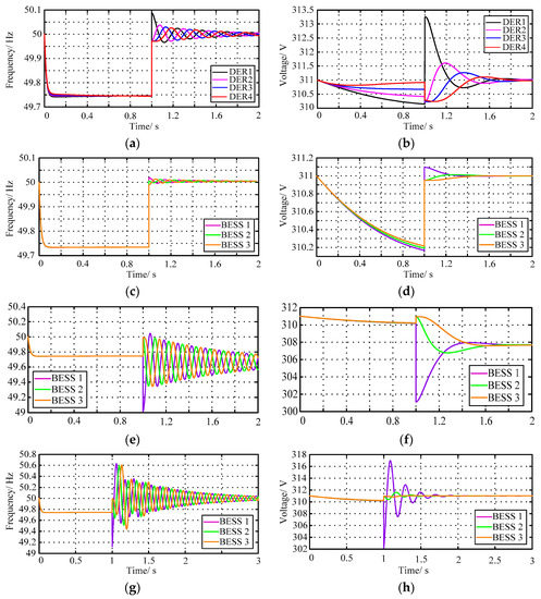
Figure 10.
Voltage and frequency variations considering the line impedance, corresponding to the BESSs and loads; (a) The frequency variations of PVs considering the line impedance of BESSs and loads; (b) The voltage variations of PVs considering the line impedance of BESSs and loads; (c) The frequency variations of BESSs under the situation 1; (d) The voltage variations of BESSs under Situation 1; (e) The frequency variations of BESSs under Situation 2; (f) The voltage variations of BESSs under the situation 2; (g) The frequency variations of BESSs under Situation 3; (h) The voltage variations of BESSs under Situation 3.
The communication topology is similar to the Figure 6, so the explanations of the Figure 9 are omitted.
The analysis is as below:
According to Figure 10a,b, under the action of droop control, the output voltage and frequency of each PV are about 59.73 Hz and 310.2 V respectively. When the secondary control is added, the controlled voltage and frequency will be adjusted to their respective reference values, i.e., 311 V and 50 Hz. Therefore, PVs can still maintain stable output. Similarly, according to Figure 10c,d, it finds that BESS can also achieve stable output under the regulation of secondary control. According to Figure 10e,f, when the disturbance data is added to the output data of BESS 1, the experimental results of secondary control will be affected. The simulation results show that when the disturbance data appear in the BESS 1, the frequency and voltage are not stable. Under the influence of the disturbance data, the two electrical quantities show a downward trend. The suppression effect of SMC on the disturbance data can be observed in Figure 10g,h. When t = 2 s, the voltage and frequency output by each BESS will appear to be chattering and tend to the reference value. Among them, the chattering situation of BESS 1 is the heaviest. However, under the action of SMC, the chattering in the controlled quantity of each BESS will be gradually reduced. Finally, the output frequency and voltage of each BESS will eventually return to the reference values.
Remark 3.
For PVs, in order to avoid the repetition of experiments in Section 5.1.1 and Section 5.1.2, we only verify in the Case 3 whether PVs can continue to maintain stable output by secondary controller.
5.1.4. Case 4: Verify the Effect of the Proposed Secondary Controller when the Load is Changed in Different Time Periods
To simulate that the load demand will be changed in different time periods, the load 2 is set to execute the following variations in Table 7.
Table 7.
The changes of load 2.
Under the corresponding operation conditions in Table 7, we have carried out two groups of simulation experiments on the MG model in Figure 5: Experiment 1. Simulate the control effect of droop control; Experiment 2. Before t = 1 s, both PVs and BESSs are controlled by droop to maintain stable output. After t = 1 s, the secondary control will be added to the MG, and then we simulate the control effect of secondary control. See the related experimental results shown in Figure 11.
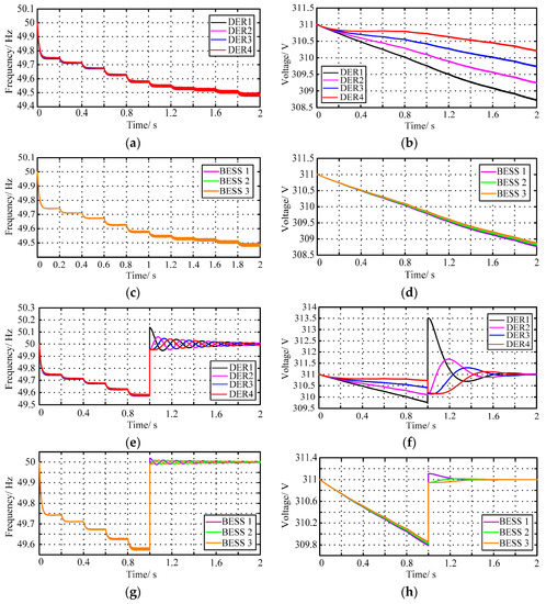
Figure 11.
Variations of output voltage and frequency of PVs and BESSs when load is changed in different time periods; (a) The frequency variations of PVs under the action of droop control; (b) The voltage variations of PVs under the action of droop control; (c) The frequency variations of BESSs under the action of drop control; (d) The voltage variations of BESSs under the action of droop control; (e) The frequency variations of PVs under the action of secondary control; (f) The voltage variations of PVs under the action of secondary control; (g) The frequency variations of BESSs under the action of secondary control; (h) The voltage variations of BESSs under the action of secondary control.
The analysis is as below: It can be seen from Figure 11a–d that under the regulation of droop control, when the load 2 is increased with time, the output voltages and frequency of PVs and BESSs will be decreased. The reason is that the energy offered by each PV and BESS is increasing, so the and in droop control are also increasing. This will cause the voltage and frequency of the output to decrease all the time. Through observing, it has found that the output frequency of PVs is reduced from 49.75 Hz to 49.5 Hz; the output voltages of PVs are reduced from 310.75 V to 308.75 V, 308.25 V, 309.75 V, and 310.25 V respectively. From Figure 11e–h, it can be observed that the outputs of PVs and BESSs are reduced because load 2 is incremental. However, after t = 1 s, the secondary control can still adjust these controlled variables to the reference values (there is a transient process between t = 1 s~t = 1.8 s). Even though load 2 is changed after t = 1 s, the outputs of PVs and BESSs are always stable. In conclusion, the effect of the proposed secondary control is not affected by the load change.
5.2. Experiment 2: Verify the Effect of the Proposed Robust Optimization Strategy
In this section, an example for a grid-connected MG is given to verify the effectiveness of the proposed method, and there are and . Moreover, so as to make the experimental model closer to the actual scene, we have designed the load as a time-varying shiftible load (i.e., the load 2) rather than a fixed load (i.e., the load 1) in Figure 5. The outputs of PV generation and load are shown in Figure 12 and the parameters of three BESSs are shown in Table 2. The maximum and minimum fluctuations of PV are and , respectively.
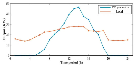
Figure 12.
The output of PV generation and load.
In particle swarm optimization, we set the quantity of particles , the maximum number of iterations of particles , and learning factors and . In order to make full use of PV power, an MPPT control strategy is adopted for PV power generation. The goal of the robust optimization framework proposed in this paper is to efficiently manage the charging and discharging status of multiple BESSs. For given loads and charging and discharging power of multi-BESSs, a common coupling point is adopted to balance the power deviation caused by the uncertainty of PV output. To improve the efficiency of multi-BESSs, an MG is allowed to sell the excessive energy to main grid when the PV power is sufficient. In this experiment, the related parameters of BESSs are as the Table 8, and the corresponding TOU price is shown in Figure 13.
Table 8.
Parameters of multi-BESSs.
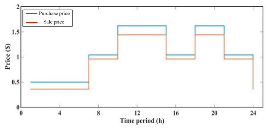
Figure 13.
TOU price.
To show the efficiency of the proposed robust optimization framework, two situations are presented in Table 9.
Table 9.
The operation process in the Experiment 2.
The PSO algorithm is used to deal with both cases. The energy dispatching scheme for Situation 1 and Situation 2 are shown in Figure 14 and Figure 15, respectively. The operation costs of Situation 1 and Situation 2 in a day are $85.6891 and $70.1305, respectively. It is clear that the cost of Situation 2 is less than that of situation 1. It is shown that the robust energy management strategy can ensure the operation cost of the system falls within a certain range, even if the uncertainty of the PV output is in the worst case. In summary, the MG operation scheme for Situation 1 has strong robustness and provides a good reference for decision makers.
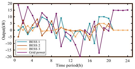
Figure 14.
Energy dispatching scheme under the situation 1.
Figure 15.
Energy dispatching scheme under the situation 2.
In Figure 14, it is observed that at the time of 1:00, 3:00, 6:00, 9:00, and 21:00–24:00, the MG will purchase more power than at other times, because the purchase prices at these moments are relatively low. In the Figure 15, it is easy to find that during the time of 5:00–7:00 and 21:00–24:00, the MG will purchase more power than at other times with the same reason as situation 1. In Figure 14 and Figure 15, it can be observed that at the time of 14:00 and 18:00, the MG will sell more power than at other times, because the sale prices at 14:00 and 18:00 are relatively high.
The SOC values of multi-BESSs in situation 1 and situation 2 are shown in the Figure 16 and the Figure 17, respectively. It is easy to see from the two figures that the SOC values of multi-BESSs are always greater than 20% and less than 80%. However, since the running cost of BESS 1 is lower than that of other BESSs but its charging and discharging power is relatively high, the SOC values of charging and discharging for multi-BESSs have different evolution from its charging and discharging power. It is clear to see that the SOC values of multi-BESSs for situation 1 are generally larger than that of Situation 2. This is because the MG needs to ensure relatively sufficient power for power unbalance by maintaining a high BESS level to improve system reliability.
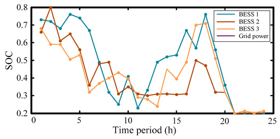
Figure 16.
SOC values of multi-BESSes under the situation 1.
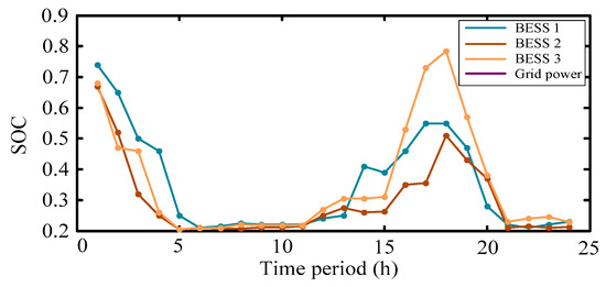
Figure 17.
SOC values of multi-BESSs under the situation 2.
Remark 4.
Regardless of the load size, the proposed energy management strategy can still be used to complete the scheduling work. The only difference may be that this will lead to different optimization strategies in each optimization time window. For example, the different relationship between PV generation and load demand will generate different generation strategies of BESSs. However, for different load conditions, the contributed methods are still applicable.
6. Conclusions
In a grid-connected MG, the integrated design method of secondary controller and robust energy management strategy for PVs is proposed. In the secondary controller, the control work is completed through using a consistency controller and event-triggered FTSMC. In the robust energy management strategy, the uncertainty of PV output, multi-BESSs, and TOU price are all considered in the optimization model. Experiment 1 showed that the control effect of the designed secondary controllers. Under this regulation, we can adjust the output voltages and frequency of DGs (including PVs and BESSs) to 311V and 50Hz in the final. Moreover, the output voltage and frequency of each DG can be also stabilized in a finite time even if there is external disturbance in the data. Meanwhile, Experiment 2 confirmed that the established model can make the energy dispatching scheme have better robustness in dealing with various PV output curves in practice, and reduce the risk of MG operation cost by sacrificing certain economy, improve the operation reliability and make decision makers have a good reference.
In the future, we will study how to maintain the stable operation of other kinds of MGs considering the uncertainly of PV and other renewable energy resources.
Author Contributions
Conceptualization, S.X.; methodology, H.S.; software, B.Z., J.Y. and T.H.; validation, A.A.; formal analysis, A.A.; data curation, H.S.; writing—original draft preparation, B.Z.; writing—review and editing, C.D. All authors have read and agreed to the published version of the manuscript.
Funding
This research was funded by the National Natural Science Foundation of China (51977197, U1766202, 51777195), Fundamental and Forecast Projects of State Grid Corporation of China “Theory Research on Response Driven Comprehensive Defense Control of Power System” (XT71-18-014), Young Elite Scientists Sponsorship Program by CAST (YESS20160157) and CSEE (JLB-2017-305).
Conflicts of Interest
The authors declare no conflict of interest.
Nomenclature
| Full Name | Abbreviation |
| Photovoltaic | PV |
| Microgrid | MG |
| Finite time sliding mode controller | FTSMC |
| Battery energy storage system | BESS |
| Particle swarm optimization | PSO |
| Distributed generator | DG |
Appendix A. The Related Simulink Model
The related explanations for the above model is as below:
The Simulink model in the experiment shown in the Figure A1 is relative to the MG system in Figure 5. It mainly includes the following parts: Four PVs and their power lines; three BESSs and their power lines; load 1; load 2; the secondary control parts on voltages of PVs; the secondary control parts on frequency of PVs; the secondary control parts on voltages of BESSs; the secondary control parts on frequency of BESSs; oscilloscopes of other electrical quantity. For PVs and BESSs, each one has its subsystem. In each subsystem, there is an inverter control system. For the secondary control parts of voltage and frequency, the corresponding oscilloscopes are used to observe their variables.

Figure A1.
The related Simulink model to experiments.
Figure A1.
The related Simulink model to experiments.

References
- Harmon, E.J.; Ozgur, U.; Cintuglu, M.H.; de Azevedo, R.; Akkaya, K.; Mohammed, O.A. The Internet of Microgrids: A Cloud Based Framework for Wide-Area Networked Microgrids. IEEE Trans. Ind. Inform. 2018, 14, 1262–1274. [Google Scholar] [CrossRef]
- Collier, S.E. The Emerging Enernet: Convergence of the Smart Grid with the Internet of Things. IEEE Ind. Appl. Mag. 2017, 23, 12–16. [Google Scholar] [CrossRef]
- Bai, X.; Qiao, W. Robust optimization for bidirectional dispatch coordination of large-scale V2G. IEEE Trans. Smart Grid 2015, 6, 1944–1954. [Google Scholar] [CrossRef]
- Anand, S.; Fernandes, B.G.; Guerrero, J.M. Distributed control to ensure proportional load sharing and improve voltage regulation in low-voltage dc microgrids. IEEE Trans. Power Electron. 2013, 28, 1900–1913. [Google Scholar] [CrossRef]
- Nasirian, V.; Davoudi, A.; Lewis, F.L.; Guerrero, J.M. Distributed adaptive droop control for dc distribution systems. IEEE Trans. Energy Convers. 2014, 29, 944–956. [Google Scholar] [CrossRef]
- Savaghebi, M.; Jalilian, A.; Vásquez, J.C.; Guerrero, J.M. Secondary control for voltage quality enhancement in microgrids. IEEE Trans. Smart Grid 2012, 3, 1893–1902. [Google Scholar] [CrossRef]
- Lu, X.; Guerrero, J.M.; Sun, K.; Vasquez, J.C. An improved droop control method for dc microgrids based on low bandwidth communication with dc bus voltage restoration and enhanced current sharing accuracy. IEEE Trans. Power Electron. 2014, 29, 1800–1812. [Google Scholar] [CrossRef]
- Tahir, M.; Mazumder, S.K. Self-Triggered Communication Enabled Control of Distributed Generation in Microgrids. IEEE Trans. Ind. Inform. 2015, 11, 441–449. [Google Scholar] [CrossRef]
- Zhou, J.; Zhang, H.; Sun, Q.; Ma, D.; Huang, B. Event-Based Distributed Active Power Sharing Control for Interconnected AC and DC Microgrids. IEEE Trans. Smart Grid 2018, 9, 6815–6828. [Google Scholar] [CrossRef]
- Zhao, L.; Zeng, B. Robust unit commitment problem with demand response and wind energy. In Proceedings of the 2012 IEEE Power and Energy Society General Meeting, San Diego, CA, USA, 22–26 July 2012; pp. 1–8. [Google Scholar]
- Valencia, F.; Collado, F.; Saez, D.; Marín, L.G. Robust Energy Management System for a Microgrid Based on a Fuzzy Prediction Interval Model. IEEE Trans. Smart Grid 2016, 7, 1486–1494. [Google Scholar] [CrossRef]
- Hussain, A.; Bui, V.H.; Kim, H.M. Robust Optimal Operation of AC/DC Hybrid Microgrids Under Market Price Uncertainties. IEEE Access 2017, 6, 2654–2667. [Google Scholar] [CrossRef]
- Nojavan, S.; Mohammadi-Ivatloo, B.; Zare, K. Optimal bidding strategy of electricity retailers using robust optimisation approach considering time-of-use rate demand response programs under market price uncertainties. IET-Gener. Transm. Distrib. 2015, 9, 328–338. [Google Scholar] [CrossRef]
- Mazidi, M.; Monsef, H.; Siano, P. Robust day-ahead scheduling of smart distribution networks considering demand response programs. Appl. Energy 2016, 178, 929–942. [Google Scholar] [CrossRef]
- Zhang, Y.; Gatsis, N.; Giannakis, G.B. Robust energy management for microgrids with high-penetration renewables. IEEE Trans. Sustain. Energy 2013, 4, 944–953. [Google Scholar] [CrossRef]
- Xiang, Y.; Liu, J.; Liu, Y. Robust energy management of microgrid with uncertain renewable generation and load. IEEE Trans. Smart Grid 2016, 7, 1034–1043. [Google Scholar] [CrossRef]
- Hussain, A.; Bui, V.H.; Kim, H.M. Robust optimization-based scheduling of multi-microgrids considering uncertainties. Energies 2016, 9, 278. [Google Scholar] [CrossRef]
- Lei, H.; Huang, S.; Liu, Y.; Zhang, T. Robust Optimization for Microgrid Defense Resource Planning and Allocation Against Multi-Period Attacks. IEEE Trans. Smart Grid 2019, 10, 5841–5850. [Google Scholar] [CrossRef]
- Yuan, W.; Wang, J.; Qiu, F.; Chen, C.; Kang, C.; Zeng, B. Robust optimization-based resilient distribution network planning against natural disasters. IEEE Trans. Smart Grid 2016, 7, 2817–2826. [Google Scholar] [CrossRef]
- Alabdulwahab, A.; Abusorrah, A.; Zhang, X.; Shahidehpour, M. Coordination of interdependent natural gas and electricity infrastructures for firming the variability of wind energy in stochastic day-ahead scheduling. IEEE Trans.Sustain. 2017, 6, 606–615. [Google Scholar] [CrossRef]
- Erdener, B.C.; Pambour, K.A.; Lavin, R.B.; Dengiz, B. An integrated simulation model for analysing electricity and gas systems. Int. J. Electr. Power Energy Syst. 2014, 61, 410–420. [Google Scholar] [CrossRef]
- Zhang, H.; Yue, D.; Xie, X. Robust Optimization for Dynamic Economic Dispatch Under Wind Power Uncertainty with Different Levels of Uncertainty Budget. IEEE Access 2016, 4, 7633–7644. [Google Scholar] [CrossRef]
- Zhang, B.; Dou, C.X.; Yue, D.; Zhang, Z.; Zhang, T. A Packet loss-dependent Event-triggered Cyber-Physical Cooperative Control Strategy for Islanded Microgrid. IEEE Trans. Cybern. 2019. [Google Scholar] [CrossRef] [PubMed]
- Fan, B.; Guo, S.L.; Peng, J.K.; Yang, Q.; Liu, W.; Liu, L. A Consensus-Based Algorithm for Power Sharing and Voltage Regulation in DC Microgrids. IEEE Trans. Ind. Inform. 2019. [Google Scholar] [CrossRef]
- Zhang, B.; Dou, C.X.; Yue, D.; Zhang, Z.Q. Response Hierarchical Control Strategy of Communication Data Disturbance in Micro-grid under The Concept of Cyber Physical System. IET-Gener. Transm. Distrib. 2018, 12, 5867–5878. [Google Scholar] [CrossRef]


© 2020 by the authors. Licensee MDPI, Basel, Switzerland. This article is an open access article distributed under the terms and conditions of the Creative Commons Attribution (CC BY) license (http://creativecommons.org/licenses/by/4.0/).