Article

A Novel Density Peak Fuzzy Clustering Algorithm for Moving Vehicles Using Traffic Radar

1
Key Laboratory of the Ministry of Education for Optoelectronic Measurement Technology and Instrument, Beijing Information Science and Technology University, Beijing 100192, China
2
School of Information and Communication Engineering, Beijing Information Science and Technology University, Beijing 100101, China
3
Beijing TransMicrowave Technology Co., Ltd., Beijing 100080, China
4
School of Computer Science and Engineering, Northeastern University, Shenyang 110004, China
*
Author to whom correspondence should be addressed.
Electronics 2020, 9(1), 46; https://doi.org/10.3390/electronics9010046
Submission received: 28 November 2019 / Revised: 23 December 2019 / Accepted: 25 December 2019 / Published: 28 December 2019
(This article belongs to the Section Computer Science & Engineering)

Abstract

:
The detection of adjacent vehicles in highway scenes has the problem of inaccurate clustering results. In order to solve this problem, this paper proposes a new clustering algorithm, namely Spindle-based Density Peak Fuzzy Clustering (SDPFC) algorithm. Its main feature is to use the density peak clustering algorithm to perform initial clustering to obtain the number of clusters and the cluster center of each cluster. The final clustering result is obtained by a fuzzy clustering algorithm based on the spindle update. The experimental data are the radar echo signal collected in the real highway scenes. Compared with the DBSCAN, FCM, and K-Means algorithms, the algorithm has higher clustering accuracy in certain scenes. The average clustering accuracy of SDPFC can reach more than 95%. It is also proved that the proposed algorithm has strong robustness in certain highway scenes.

1. Introduction

Radar is an important part of the contemporary intelligent transportation system [1,2,3]. Multi-target tracking with radar is also a hot issue in intelligent transportation research [4,5,6]. By tracking passing vehicles, risky driving behavior can be predicted and an early warning signal can be issued [7,8]. Vehicle tracking helps to reduce the occurrence of traffic accidents, and also helps the development of intelligent transportation [9]. Currently, there are many image-based multi-target tracking algorithms [10]. However, these methods do not show good adaptability in the actual traffic scenes. Because they cannot adapt to the effects of weather, environment, and light [11,12]. Since radar signals can be well adapted to complex scenes [13], more and more researchers are beginning to use millimeter-wave radar to solve multi-target tracking problems [14,15] in traffic.
The sampling points collected by the radar are scattered, and doped with noise [16]. Therefore, clustering sampling points before the target tracking can promote better tracking of the targets [17]. The experimental scene of this paper is a straight four-lane highway. In this scene, vehicles in the adjacent lanes may be close to each other during driving. At this time, the sampling points of the vehicles may be close together and cover each other. Current clustering algorithms cannot distinguish adjacent targets and covered targets well, and real-time performance is not good as well. Therefore, the purpose of this paper is to improve the cluster accuracy of adjacent vehicle sampling points in highway scenes.
There are a lot of clustering algorithms at present. For example, partition-based clustering algorithms [18], hybrid density clustering algorithms, graph clustering algorithms, fuzzy clustering algorithms, and so on. The classic one in the partition-based clustering algorithm is the K-Means clustering algorithm [19,20]. This algorithm has a wider application and higher efficiency, but it also has obvious limitations. The algorithm must determine a cluster center of each cluster in advance. The choice of this cluster center determines the quality of the clustering results. The algorithm is sensitive to abnormal sample points and can only process numerical data sets. The FCM (Fuzzy C-Means) algorithm [21,22,23] is a widely used clustering algorithm applied to the field of image segmentation. The algorithm uses a membership degree to determine the similarity of sample points. It is a fuzzy clustering method based on the objective function [24,25,26]. The DBSCAN (Density-Based Spatial Clustering of Applications with Noise) algorithm is a density-based partitioning clustering method. It treats the data set as a collection of several high-density clusters separated by low-density regions. The main feature of this method is that clusters of any shape can be identified [27].
Many researchers have made many improvements to existing algorithms. The K-MODES algorithm proposed by Nguyen [28] overcomes the shortcomings of the K-Means algorithm that can only process numerical data. The K-MEDOIDS algorithm does not calculate the cluster center but directly represents a cluster to represent the cluster, which can effectively handle abnormal data [29,30]. Bezdek’s research team improved the FCM algorithm and they globally optimized the fuzzy objective function [31]. Birant et al. improved the DBSCAN algorithm and proposed a new ST-DBSCAN (Spatial-Temporal DBSCAN) algorithm. The algorithm can find clusters of clusters in non-spatial values, spatial values, and temporal values [32]. In 2014, density peak fast clustering was a new efficient clustering algorithm proposed by Italian researcher Rodriguez et al. [33]. The main idea of the algorithm is that the cluster center has a higher density than the neighborhood, and the cluster center has a relatively large distance from the high-density point.
For the inaccurate clustering results of adjacent vehicles in the highway scenes, this paper constructs a spindle-based density peak fuzzy clustering (SDPFC) system using traffic radar. Our optimization goal is to increase the clustering accuracy of adjacent vehicles in highway scenes. In order to increase the clustering accuracy, the cluster centers and the number of clusters are calculated by the initial clustering algorithm based on density peak. The final clustering result is calculated by the fuzzy clustering algorithm based on spindle update. The main diagram of the spindle-based density peak fuzzy clustering system using traffic radar is shown in Figure 1. The experimental results show that the SDPFC algorithm has advantages in clustering accuracy. In summary, the contributions of this paper can be summarized as follows:
  • This paper proposes a spindle-based density peak fuzzy clustering (SDPFC) algorithm. The algorithm is divided into two parts: initial clustering and quadratic correction clustering. The initial clustering is to determine the cluster center and the number of clusters by finding the density peak. The quadratic correction clustering is to correct the clustering results by iterative updating of the fuzzy matrix and the spindle. In this way, the problem of inaccurate clustering of adjacent vehicles is solved.
  • SDPFC overcomes the defect that the traditional fuzzy algorithm is not ideal for non-spherical sample set clustering. To improve the accuracy of the clustering algorithm, this paper changes the concept of iteratively updating the cluster center to the update of the spindle. In actual traffic scenes, SDPFC is more reasonable than other commonly used algorithms.
  • In order to accelerate the clustering algorithm, the randomly generated initial cluster center is no longer used in this paper. Instead, the ideal initial cluster center is calculated by finding the density peak. In this way, the structure of the SDPFC algorithm is optimized. Since the ideal initial cluster center is close to the real target cluster center, the optimization algorithm greatly reduces the number of iterations.
The rest of this paper is organized as follows. In Section 2, we introduce the data acquisition method of multi-target traffic microwave radar and feature data extraction for vehicles. The data collected include distance, velocity, and angle. In Section 3, the clustering algorithms related to this paper will be introduced. In Section 4, the spindle-based density peak fuzzy clustering algorithm is explained. Section 5 describes the experimental results of several real highway scenes, the performance of several algorithms is compared, and the applicability of the algorithm is discussed. Section 6 summarizes this paper.

2. Radar Signal Preprocessing

The traffic scene in this paper is a straight four-lane highway, as shown in Figure 2. On the highway, safe driving is significant. Therefore, not only the driver’s driving experience but also the strict supervision of the relevant departments are required to avoid accidents [34]. On the highway, long-term cross-lane driving is extremely dangerous. However, in practice, it is found that, if two vehicles are driving in parallel when the driving distance is too close, the sampling points will gather and cover each other [35]. At this time, it is usually judged that this is a car driving on the lane line. This will result in erroneous tracking of vehicle targets. At the same time, false alarms will be issued and the vehicle will be photographed, which will cause the owner to accept the penalty. These problems can result in wasted resources. Therefore, the algorithm in this paper is to solve the problem of inaccurate clustering results of the adjacent vehicle in highway scenes.
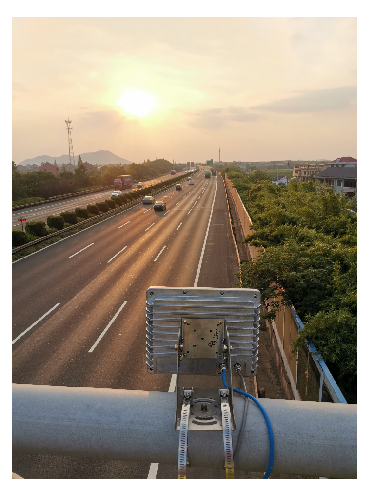
The radar systems used in this paper mainly include a radar, camera, and alarm. It is mounted on a beam 7 m above the ground on the side of the lane. In addition, it is capable of monitoring vehicle targets in the longitudinal direction between 50 and 300 m and in the lateral 4–5 lanes. The radar has the ability to monitor passing vehicles on the road. The traffic radar used in this paper has high measurement accuracy. In a distance range of about 150 m, the distance measurement error is about 0.15 m, and the angle measurement error is about 0.1 degrees. By processing the data collected by the radar, information such as the position and speed of each vehicle can be obtained, thereby tracking the trajectory of all vehicles in the current monitoring scene.
The raw data received by the radar are a time-domain signal, which needs to be converted by the following steps:
  • Step 1: Receive an echo signal from the radar at the current time;
  • Step 2: Transform the echo signal from the time domain to the frequency domain by using FFT (Fast Fourier Transform);
  • Step 3: Determine the distance between the vehicle target and the radar-based on the spectrum information of the echo signal by Formula (1):
    R = c T Δ f 2 B ,
    where R is the distance from the radar to the target vehicle; c is the speed of light; T is the period of the transmitted signal; Δ f is the difference frequency between the transmitted signal and the received signal; B is the signal bandwidth;
  • Step 4: According to the spectrum information of the echo signal, the angle between the target vehicle and the radar is determined by Formula (2):
    θ = arcsin ( λ 6 π · l = 1 3 Δ φ l d l ) ,
    where θ represents the angle between the target and the normal direction of the radar; λ represents the wavelength of the electromagnetic wave emitted by the antenna; Δ φ l represents the phase difference between the l th antenna and the l + 1 th antenna; d l represents the distance between the l th antenna and the l + 1 th antenna;
  • Step 5: According to the distance and angle between the target vehicle and the radar, the two- dimensional coordinate position ( x , y ) of the target vehicle in the plane rectangular coordinate system is determined by Formulas (3) and (4):
    x = R · sin θ ,
    y = ( R · cos θ ) 2 h 2 ,
    where h represents the height of the radar from the road plane.
This paper establishes a plane rectangular coordinate system in the road plane, and the origin of the plane rectangular coordinate system is the projection position of the radar on the road plane. By transforming the coordinate ( R , θ ) in the polar coordinate system to the coordinate ( x , y ) of the plane rectangular coordinate system, the vehicle trajectory can be visually displayed. The algorithm in this paper mainly uses the coordinate z = ( x , y ) of the sampling point as input information.

3. Previous Works

3.1. DBSCAN Clustering Algorithm

DBSCAN is a density-based spatial clustering algorithm [36]. The algorithm divides a set of sample points with sufficient density into one cluster [37], and finds a class of arbitrary shape in a set of spatial sample points with noise. The algorithm defines the cluster as the largest set of points connected by density [38]. Before describing the algorithm, we first define several related concepts:
  • σ -Neighborhood: The set of sample points within a given object radius σ is called the σ -Neighborhood of the object in dataset D, denote by N σ z i = z j D | d i s t z i , z j σ .
  • Core object: For any object z i D , if there are at least min p t s objects in its σ -Neighborhood that is, if | N σ z i | min p t s , then z i is the core object.
  • Directly Density-Reachable: An object z j is said to be directly density-reachable from an object z i if z j is within the σ -Neighborhood of z i , and z i is a core object.
  • Density-Reachable: z j is density-reachable to z i if there exists an object chain p 1 , p 2 , p T , such that p 1 = z j , p T = z i and p k + 1 is directly density-reachable from p k .
  • Density-Connected: An object z j is density-connected to object z i with respect to σ and min p t s if there exists a core object z k such that both z j and z i are directly density-reachable from z k with respect to σ and min p t s .
The flow of DBSCAN clustering algorithm as shown in Algorithm 1:
Algorithm 1 DBSCAN
Require: sample points z.
Ensure: cluster center z i , and l a b e l .
1:
initialization σ -Neighborhood, and min p t s ;
2:
repeat
3:
traverse all sampling points z and determine whether the point is a core object that satisfies the σ -Neighborhood;
4:
until all sample points are traversed, and find all core object sets that satisfy the σ -Neighborhood;
5:
repeat
6:
choose a core object, find all the density-Reachable sample points and generate clusters;
7:
remove the density-reachable sample points found in the previous step from the remaining core objects;
8:
until core objects are traversed or removed;
9:
return: cluster center z i and l a b e l ;
The DBSCAN clustering algorithm can cluster dense sample points of any shape and can be used in traffic scenes. However, the algorithm needs to coordinate the neighborhood radius and the sample number threshold to find the optimal solution in the current scene. This is more complicated for the user. In addition, in the traffic scene solved in this paper, the radar sampling points of adjacent vehicles are close to each other and the density is similar. The DBSCAN clustering algorithm cannot solve the problem of distinguishing adjacent vehicles in traffic scenes.

3.2. FCM Clustering Algorithm

The FCM algorithm is based on a data clustering method optimized for the objective function [39]. The clustering result is the degree of membership of each data point to the cluster center, and the degree of membership is represented by a numerical value [40,41]. The FCM algorithm is an unsupervised fuzzy clustering method, and no human intervention is needed in the algorithm running process after manually determining the initial parameters [42].
Taking the sample points set of this paper as an example, the sampling points are z = z j , j = 1 , 2 , , m k . If the sampling points are divided into cluster i, the cluster center is i c , i = 1 , 2 , , I . Each sample j belongs to the cluster i with a membership of μ i j , so the objective function of the FCM is defined as:
J = i = 1 I j = 1 k μ i j m z j i c 2 .
The sum of the membership degrees of each sample j belonging to a certain cluster i shall be 1:
i = 1 I μ i j = 1 , j = 1 , 2 , , k .
The Lagrange Multiplier Method is used to put the constraint into the objective function, and then expand to get Formula (7):
J = i = 1 I j = 1 k μ i j m z j i c 2 + λ 1 ( i = 1 I μ i j 1 ) + + λ j ( i = 1 I μ i j 1 ) + + λ k ( i = 1 I μ i k 1 ) .
The extreme value of J is required. In addition, make the partial derivative result of μ i j and i c be 0:
J μ i j = m z j i c 2 μ i j m 1 + λ j = 0 , J i c = j = 1 k ( 2 μ i j m ( z j i c ) ) = 0 .
Solve Formula (8):
μ i j = 1 n = 1 I z j i c 2 z j i n 2 2 m 1 , i c = j = 1 k μ i j m j = 1 k μ i j m z j .
The flow of the FCM clustering algorithm is as shown in Algorithm 2:
Algorithm 2 FCM
Require: sample points z.
Ensure: cluster center i c , and l a b e l .
1:
initialization: Number of clusters i, weighted index m, termination error η , and membership matrix μ i j ;
2:
repeat
3:
calculate the cluster center position i c according to Formula (9);
4:
update membership matrix μ i j according to new cluster center and Formula (9);
5:
until the objective function J tends to be stable according to the condition in Formula (10);
6:
return: cluster center i c and l a b e l ;
ε = i = 1 I j = 1 k ( new μ i j μ i j ) < η .
The FCM clustering algorithm calculates the membership degree of each sample point. If a sample point has an absolute advantage in the membership degree of a certain cluster, it is a very safe practice to assign the sample point to this cluster. The algorithm is highly accurate. However, some parameters need to be set in the algorithm, the number of clusters i, the weighted index m, and the termination error η . If the initialization of the parameters is not appropriate, it may affect the correctness of the clustering results. Secondly, when the data sample set is large and the number of features is large, the real-time performance of the algorithm is not good. In addition, in the traffic scene of this paper, the radar sampling points of adjacent vehicles are close, and FCM cannot solve the problem of distinguishing adjacent vehicles.

4. The Spindle-Based Density Peak Fuzzy Clustering (SDPFC) Algorithm

The SDPFC algorithm proposed in this paper is characterized by the idea of using quadratic clustering to correct clustering results. The cluster center of each cluster and the number of clusters are obtained by the initial clustering algorithm based on the density peak [43]. Then, the clustering result of the initial cluster is corrected by the fuzzy clustering algorithm based on the spindle update, and the final clustering result is obtained. The combination of these two clustering ideas will be explained in this section.

4.1. Initial Clustering Algorithm Based on Density Peak

Taking the sampling points of the paper as an example, the sample points set S = z i i = 1 n to be clustered. I S = 1 , 2 , , n is the corresponding indicator set [44]. Calculate the Euclidean distance d i j between all sample points, as shown in Formula (11). Thus, the number of d i j is n n 1 2 :
d i j = d i s t z i , z j .
All d i j are sorted in ascending order, and a percentage parameter p is set, then the truncation distance d t is defined as the r th d i j , where r is calculated by Formula (12) and r o u n d represents rounded off. In the experimental environment of this paper, the sampling points are relatively close, so p in this article is chosen to be 2%. Users can modify p according to their own experimental environment. The larger the p that is selected, the more clusters are filtered out. Therefore, p should be determined through the experimental environment:
r = r o u n d n n 1 2 p .
The density ρ i of each sample point z i is calculated by Formula (13):
ρ i = j I S \ i e d i j d c 2 .
For each sample point z i , find all sample points z j that are denser than the sample point z i and select the smallest d i j , denoted as δ i . If the opposite is true, select the largest d i j and record it as δ i . The significance of this is that the characteristics of ρ i and δ i can be used to determine whether the sample point is the cluster center. The selection method of δ i is as shown in Formula (14):
δ i = min j I S i d i j , I S i , max j I S d i j , I S i = ,
where represents the empty set, and the expression of the indicator set is as shown in formula (15):
I S i = k I S : ρ k > ρ i .
You need to set the threshold parameter to find the center point of each type of sample, set the density threshold to ρ 0 , and the distance threshold to δ 0 . If ρ i > ρ 0 and δ i > δ 0 of the sample point z i , the sample point z i is considered to be the cluster center of a certain cluster.
As shown in Figure 3, this diagram is called a decision diagram. It can be clearly seen in the figure that the colored elements in the upper right corner have a larger ρ and δ . This means that they are more likely to be the center of the cluster. With the decision graph, we can easily determine which points qualify as the center point and which points are not qualified by defining the density threshold ρ 0 and the distance threshold δ 0 according to the experimental environment.
Define m j j = 1 n c as the number of the corresponding sample point of each cluster center that is, z m j represents the center of the j th cluster. In addition, define c i i = 1 n as the sample point clustering label, that is, c i indicates that the i th sample point in S belongs to the c i th cluster. Thus, c i satisfies the logic of Formula (16).:
c i = k , i f ( z i i s t h e c l u s t e r c e n t e r a n d b e l o n g s t o t h e k t h c l u s t e r ) , 1 , o t h e r w i s e .
Define n i i = 1 n as the number of nearest sample points in the sample points with the local density greater than z i in the S, as defined by Formula (17):
n i = arg min j I S i d i j , I S i , 0 , I S i = .
Using the attributes defined by Formula (17), the sample points are processed one by one by local density—the highest density sample point except for the center point. It falls into the cluster to which it is close. This way of processing one by one is much faster than loop iteration.
Define h i i = 1 n as the identity of the cluster core and cluster halo. The cluster core indicates that the local density is large, corresponding to the core part of the cluster. The cluster halo is denser and corresponds to the edge of the cluster. The value of h i is as shown in Formula (18):
h i = 0 , z i c l u s t e r c o r e , 1 , z i c l u s t e r h a l o .
If n c > 1 , an average local density upper bound ρ i b i = 1 n c is generated for each cluster. For a fixed cluster, first determine its boundary area, which consists of sample points: they belong to the cluster itself, but within a range that does not exceed d c ; sample points belong to other clusters. Using the cluster in the boundary area, an average local density can be calculated to distinguish between the cluster core and the cluster halo.
The average density is calculated as shown in Formula (19):
ρ ¯ = ρ i + ρ j 2 .
The upper bound of the average local density is obtained by Formula (20):
ρ c i b = ρ ¯ , ρ ¯ > ρ c i b , ρ c j b = ρ ¯ , ρ ¯ > ρ c j b .
The value of h i is as shown in Formula (21):
h i = 1 , ρ i < ρ c i b , h i = 0 , o t h e r w i s e .
The general calculation process of the initial clustering algorithm based on the density peak is described below. Firstly, after initialization and preprocessing, calculate the Euclidean distance d i j between all sample points and determine the cutoff distance d t according to Formula (12). Calculate ρ i and δ i for each sample point. Secondly, determine the cluster center and initialize the label according to Formula (16). The cluster centers and their numbers of the cluster are finally obtained. Thirdly, the sample points that are not cluster centers are categorized until the categorization process for each sample point is completed. Finally, if n c > 1 , the sample points in each cluster are further divided into cluster core and cluster halo.
The flow of initial clustering algorithm based on density peak as shown in Algorithm 3:
Algorithm 3 Initial clustering algorithm based on density peak
Require: sample points z.
Ensure: cluster center z i , the number of clusters i, and l a b e l .
 1:
initialization: cutoff distance d t , cluster center number i, density threshold ρ 0 , and distance threshold δ 0 ;
 2:
  for i 1 t o n d o
 3:
    for j 1 t o n d o
 4:
      calculate the Euclidean distance d i j between all sample points and calculate ρ i and δ i for each sample point.
 5:
    end for
 6:
  end for
 7:
repeat
 8:
get the cluster center z i and its number i;
 9:
until classify all sample points that are not cluster centers;
10:
  for i 1 t o n d o
11:
    if n c > 1 then
12:
      the sample points in each cluster are further divided into cluster core and cluster halo according to Formula (21);
13:
      end if
14:
  end for
15:
return: cluster center z i , the number of clusters i, and l a b e l ;
Taking a scene on the highway as an example, the clustering result of the initial cluster is shown in Figure 4. The horizontal and vertical coordinates in the figure indicate the distance. Each point in the graph represents each sample point. This graph is an image generated from the distance between sample points. Therefore, the distance between each sampling point in the graph is real, but their coordinate positions are not real positions. This graph is only used to clearly show the cluster centers and the number of clusters.

4.2. Fuzzy Clustering Algorithm Based on Spindle Update

According to the results obtained in the previous section, the correction after initial clustering is performed to obtain the final clustering result. The results of the previous section used in this section are: position coordinate information of all sampling points, cluster centers, and the number of clusters. Define i = 1 , 2 , , I represents the i th cluster, and z 0 ( i ) for the i th cluster center.
The radar used in the article is a traffic scene monitoring radar that is mounted above the side of the lane. Therefore, the positional relationship between the radar and the lane is unchanged. The normal driving situation of the vehicle is that the vehicle travels forward between the lane lines. In addition, it is illegal to travel across the lane for a long time. Whether driving normally or across the lane, the vehicle travels in a direction parallel to the centerline of the lane. Therefore, based on the results obtained in the previous section, we use the straight line passing through the cluster center and parallel to the centerline of the lane as an important basis to correct the results of the initial clustering, so as to obtain better clustering results. We traveled on the road in advance through a dedicated calibration vehicle. The collected lane centerline is used as the initial spindle. Record the slope of the initial spindle as a 0 .
According to the above characteristics, the initial spindle is constructed based on the center of each cluster and the centerline of the lane. The initial spindle is a straight line parallel to the centerline of the lane and passing through the cluster center. Express the spindle of cluster i as L c ( i ) , and its expression is: y = a ( i ) x + b ( i ) , where i = 1 , 2 , , I represents the i th cluster and j = 1 , 2 , , k represents the j th sample point, and the value of k is the number of all sample points except the cluster center. The expression with a 0 as the slope and the initial spindle passing through the cluster center z 0 ( i ) = ( x 0 ( i ) , y 0 ( i ) ) of each cluster is:
y = a 0 ( i ) x + b 0 ( i ) .
The position coordinates of the sample points obtained in the plane rectangular coordinate system are defined as:
z j = ( x j , y j ) .
In the text, the distance between the j th sample and the spindle of the i th cluster is expressed by Formula (24), and its value is D j ( i ) :
z j L c ( i ) .
Define the objective function T, and the expression is as shown in Formula (25):
T = i = 1 I j = 1 k B i j m D j ( i ) 2 ,
where B represents a fuzzy matrix, indicating the confidence that the sample points belong to a certain cluster. m represents the factor of membership, that is, the weight. This value can be determined by the user. The constraint of B is:
i = 1 I B i j = 1 , j = 1 , 2 , , k .
In order to achieve the optimal solution of the objective function, it is necessary to make T obtain a minimum value under the constraint condition. The Formula (25) is expanded using the Lagrange method:
T = i = 1 I j = 1 k B i j m D j ( i ) 2 + λ 1 ( i = 1 I B i j 1 ) + + λ j ( i = 1 I B i j 1 ) + + λ k ( i = 1 I B i k 1 ) .
The proof that Formula (25) is a continuously differentiable function is shown in Appendix A. In addition, the result of the partial derivative of T is:
T B i j = m D j ( i ) 2 B i j m 1 + λ j = 0 .
Calculate B i j :
B i j m 1 = λ j m D j ( i ) 2 B i j = λ j m 1 m 1 1 ( D j ( i ) 2 ) 2 m 1 ,
where B i j represents the membership between the j th sampling point and the i th clustering center. Substitute B i j into Formula (26):
λ j m 1 m 1 n = 1 I 1 ( D j ( n ) 2 ) 2 m 1 = 1 ,
where n represents the n th cluster center. Simplify Formula (30):
λ j m 1 m 1 = 1 n = 1 I 1 ( D j ( n ) 2 ) 2 m 1 .
Substitute Formula (31) into Formula (29):
B i j = 1 n = 1 I 1 ( D j ( n ) 2 ) 2 m 1 1 ( D j ( i ) 2 ) 2 m 1 = 1 n = 1 I D j ( i ) 2 D j ( n ) 2 2 m 1 .
It can be clearly seen from Formula (32) that, if you want to obtain the membership B i j between the j th sample point and the i th cluster center, you need to calculate the ratio of the distance from the sample point to a cluster center to the sum of the distances from the sample point to all cluster centers. The higher the ratio, the higher the membership. The Formula (32) is the updated formula for B i j . While updating the fuzzy matrix B , the spindle needs to be updated.
Spindle update process:
The straight line formula of the spindle is: y = a ( i ) x + b ( i ) . The sample points are: z j : ( x 1 , y 1 ) , ( x 2 , y 2 ) , , ( x m k , y m k ) .
D j ( i ) is the distance from the sample point to the spindle of the i th cluster:
D j ( i ) = a ( i ) x j y j + b ( i ) a ( i ) 2 + 1 , y 0 ( i ) d c sin arctan a ( i ) y j y 0 ( i ) + d c sin arctan a ( i ) , x j ( i ) 2 x j 2 + y j ( i ) 2 y j 2 , o t h e r w i s e .
Next, we need to reconstruct the clusters of the sample points. If the ordinate of the sample point is within the distance d c from the ordinate of the cluster center of a certain cluster, calculate the distance from the sample point to the spindle. Otherwise, calculate the Euclidean distance of the sample point to the cluster center. When D j ( i ) is the minimum value, it is judged that the sample point is classified into the i th cluster.
The following update processes take place within the new clusters of reconstructing. Taking a certain cluster as an example, the spindle is updated in the following ways.
Define δ as the sum of the squares of the errors. The expression is:
δ = j = 1 m D j = j = 1 m ( y j a x j b ) 2 ,
where m represents the number of sample points outside the center of a certain cluster. Calculate the partial derivative of a, b respectively:
δ a = 2 ( j = 1 m x j y j b j = 1 m x j a j = 1 m x j 2 ) , δ b = 2 ( j = 1 m y j j = 1 m b a j = 1 m x j ) , δ a = 2 ( j = 1 m x j y j b m x ¯ a j = 1 m x j 2 ) , δ b = 2 ( m y ¯ b m a m x ¯ ) .
Let the two formulas of Formula (35) be 0, and get:
a = j = 1 m ( x j x ¯ ) ( y j y ¯ ) j = 1 m ( x j x ¯ ) 2 , b = y ¯ a x ¯ .
The flow of the fuzzy clustering algorithm based on spindle update as shown in Algorithm 4:
Algorithm 4 Fuzzy clustering algorithm based on spindle update
Require: sample point set z j ( i ) , the number of clusters i, cluster center z 0 ( i ) .
Ensure: cluster center z 0 ( i ) , and l a b e l .
1:
initialization: weighted index m, membership matrix B , spindle slope a 0 , spindle of each cluster L c ( i ) , and termination error η ;
2:
repeat
3:
update membership matrix B according to Formula (32);
4:
update the spindle of each cluster according to Formula (36);
5:
until the objective function T tends to be stable according to the condition in Formula (37);
6:
return: cluster center z 0 ( i ) and l a b e l ;
V = i = 1 I j = 1 k ( new B i j B i j ) < η .
The initial clustering results of the previous section are subjected to quadratic modified clustering, and the final clustering result is shown in Figure 5.

5. Comparison of Experimental Results

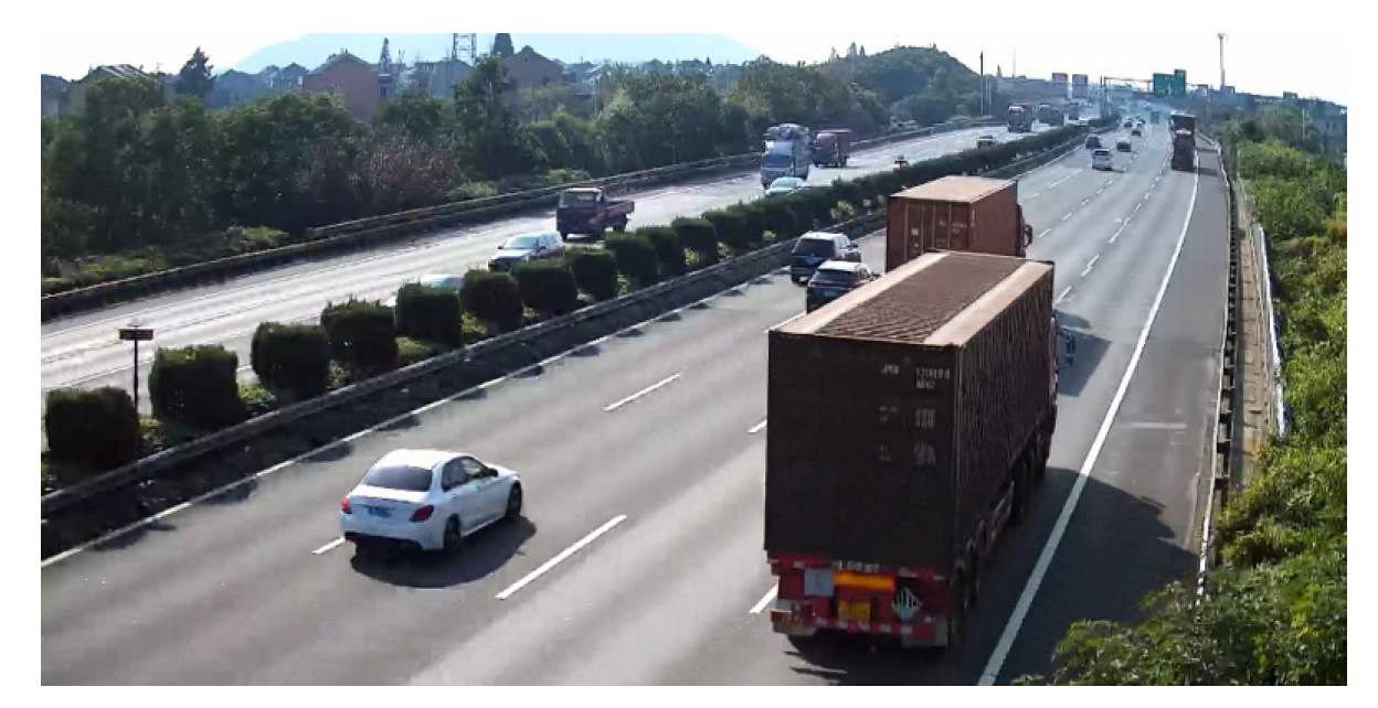
The experimental scene in this paper is a straight four-lane highway scene with the radar mounted above the side of the lane, as shown in Figure 6. The vehicles on the highway are characterized by a fast speed and large distance between front and rear. However, during the driving process, the approach of the vehicle will occur, which will cause the radar sampling points to approach and cover each other. The current commonly used clustering algorithms cannot accurately distinguish between adjacent and covered vehicle targets. The spindle-based density peak fuzzy clustering algorithm proposed in this paper can better solve the clustering problem of adjacent vehicles in this scene.
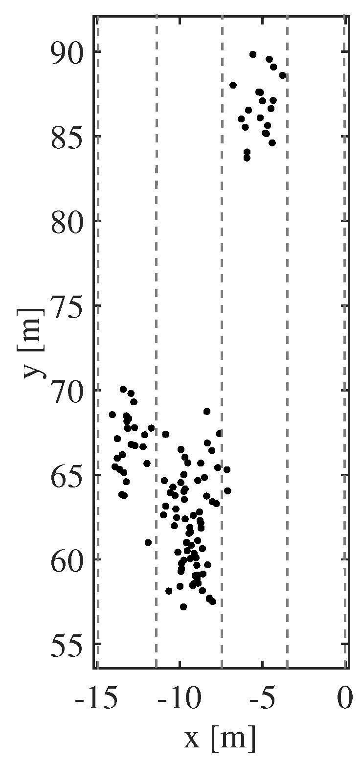
Scene 1: There are three vehicles with a relatively short distance on the straight four-lane highway. Among them, two large vehicles have a lateral distance that is very close to each other and the other one is farther away from the two cars, as shown in Figure 7. At this time, the radar returns a total of 117 valid sampling points, and the distribution of sampling points is shown in Figure 8.
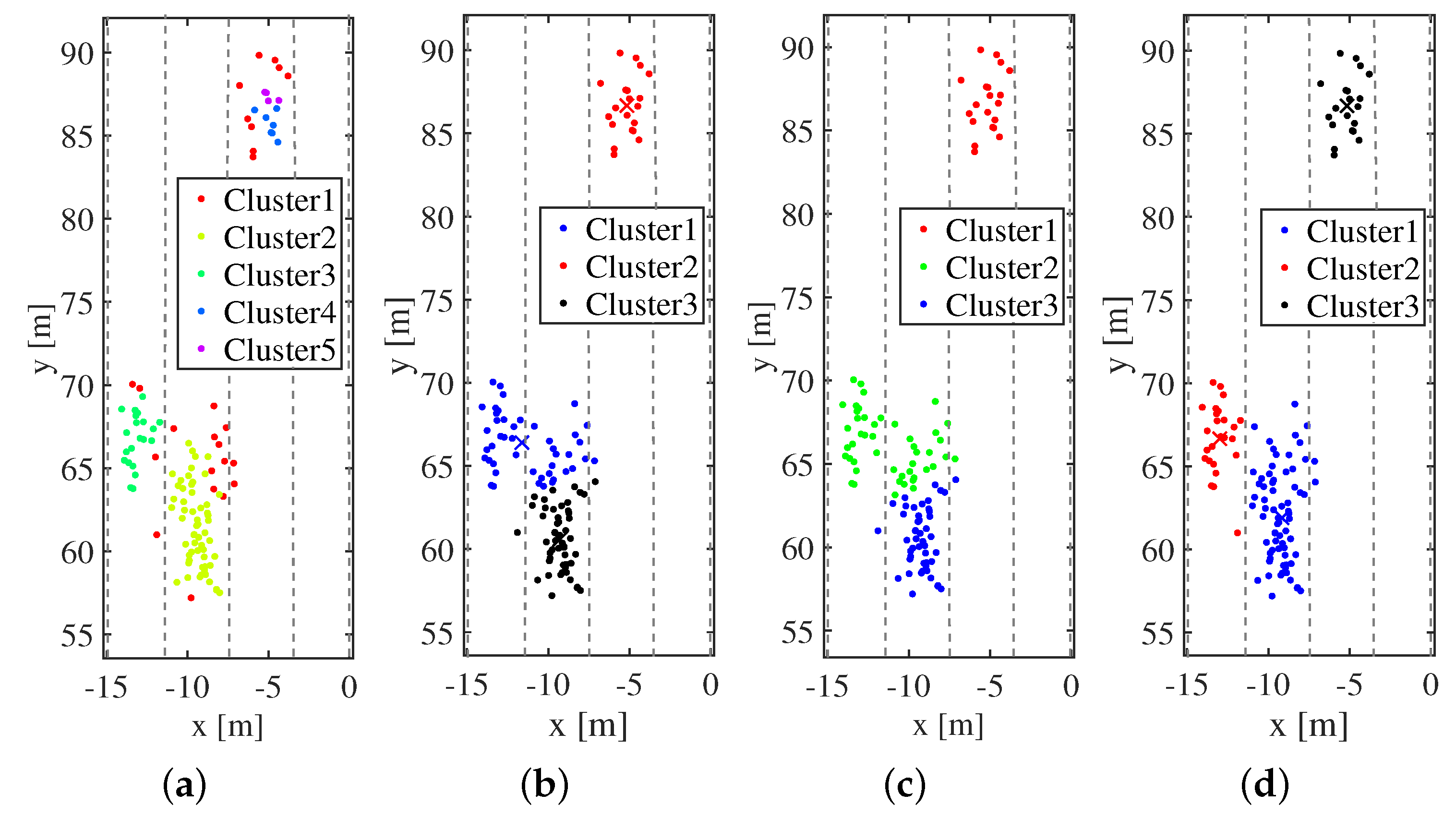
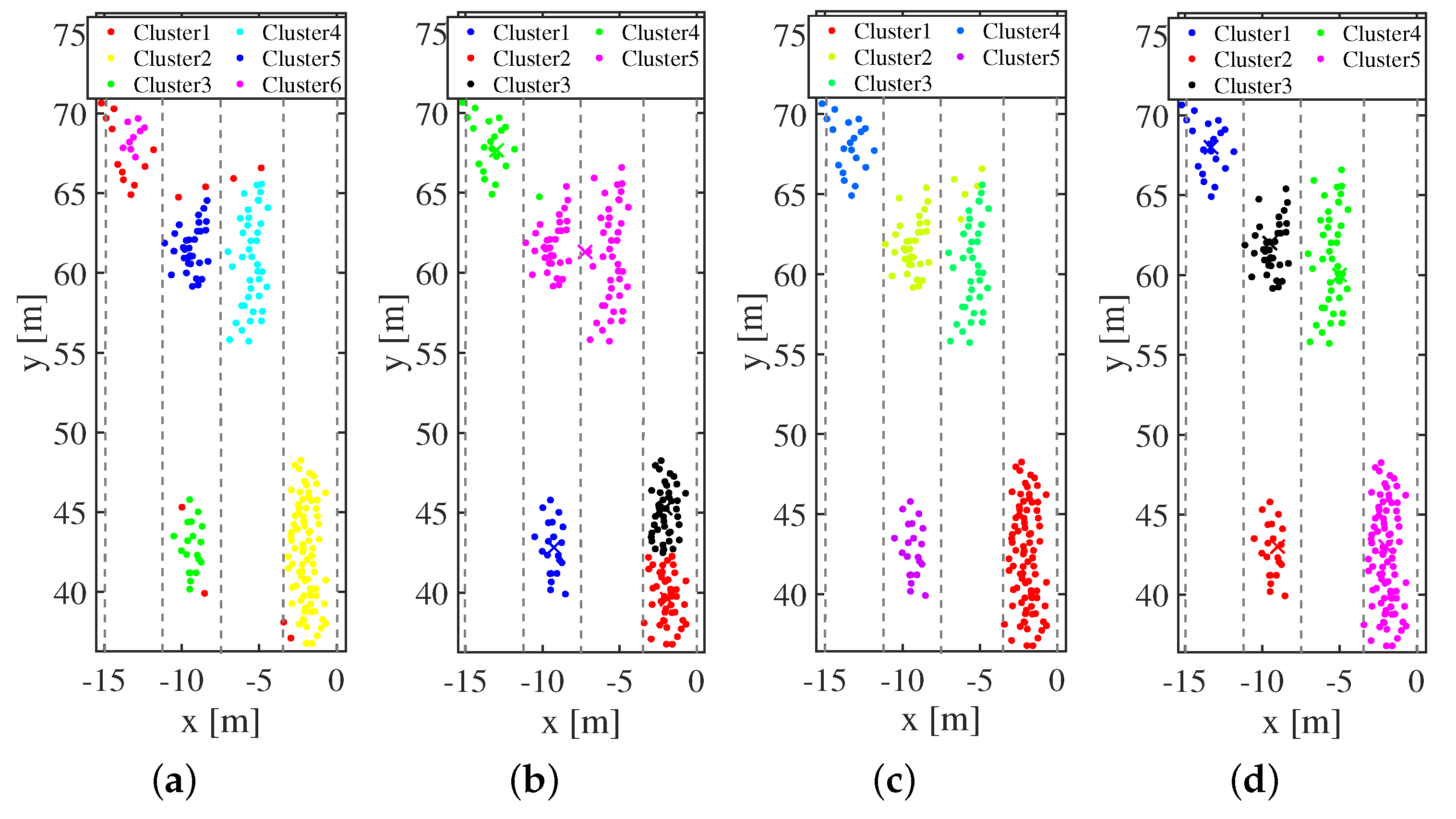
The comparison of clustering results of various algorithms in this scene is shown in Figure 9.
In this scene, two large cars cover each other, resulting in an uneven distribution of sampling points. The DBSCAN algorithm classifies by density and results in a large number of clusters. The iterative update of the fuzzy matrix and the cluster center by the FCM algorithm cannot solve the problem of distinguishing adjacent targets well. The K-Means algorithm does not classify well for adjacent sample points. The clustering results obtained by the SDPFC algorithm in this paper can correspond well to the real scene. Compared with the results of other algorithms, the conclusion of the new algorithm is better.
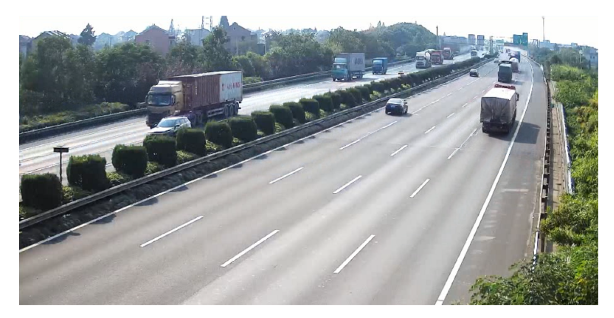
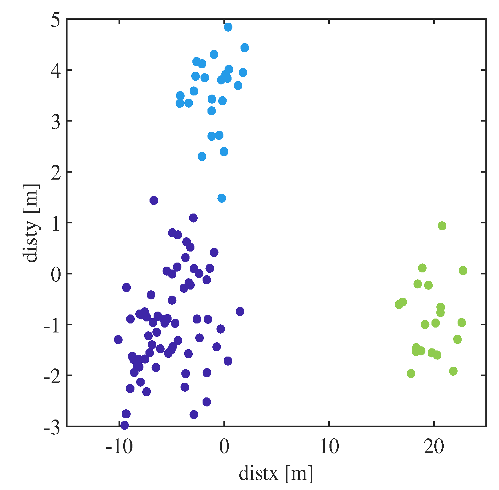
Scene 2: There are three vehicles with a close driving distance on the straight four-lane highway. The lateral distance between the two vehicles is very close and the large vehicle covers the small vehicle. The other one is farther away from the two vehicles, as shown in Figure 10. At this time, the radar returns a total of 115 valid sampling points, and their distribution is shown in Figure 11.
The comparison of clustering results of various algorithms in this scene is shown in Figure 12.
In this scene, a large car covers a small car, resulting in fewer sample points for the small car. The DBSCAN algorithm classifies by density and results in a large number of clusters. The iterative update of the fuzzy matrix and the cluster center point by the FCM algorithm cannot solve the problem of distinguishing adjacent targets well. The K-Means algorithm does not classify well for adjacent sample points. The clustering results obtained by the density peak fuzzy clustering algorithm in this paper can correspond well to the real scene. Compared with the results of other algorithms, the conclusion of the new algorithm is better.
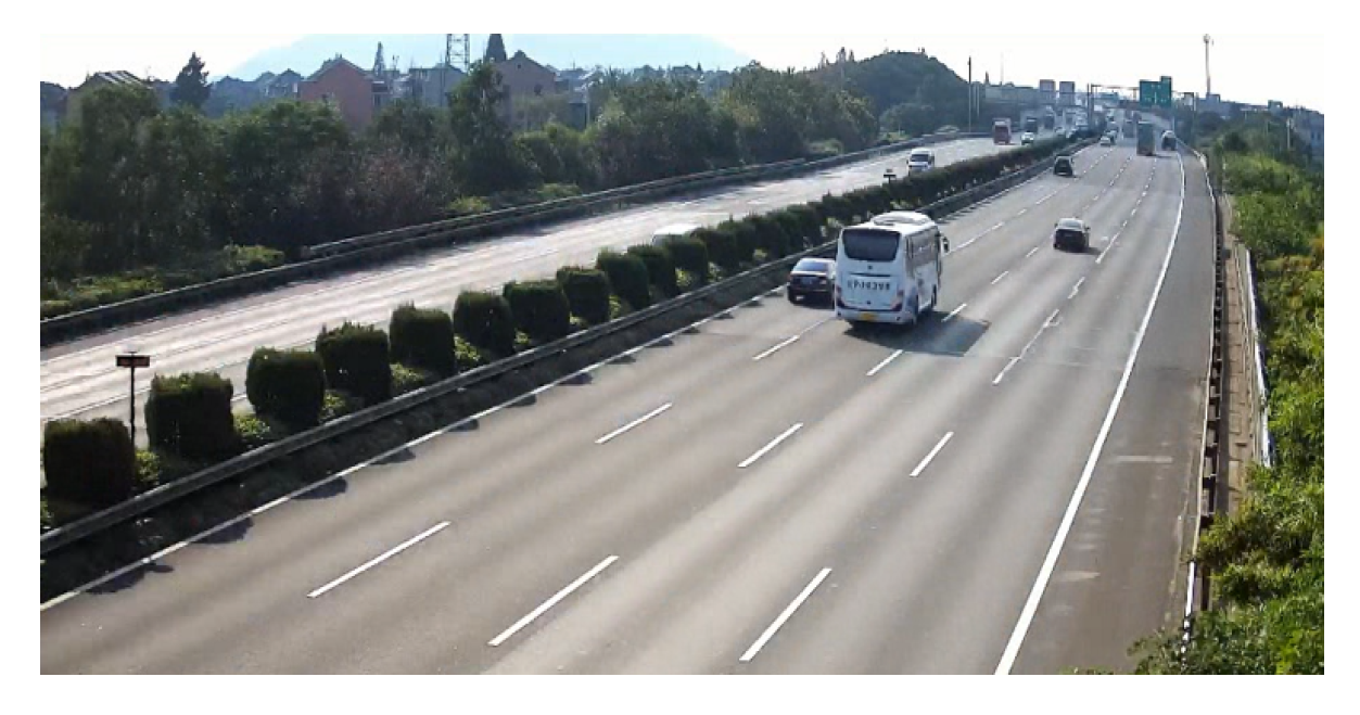
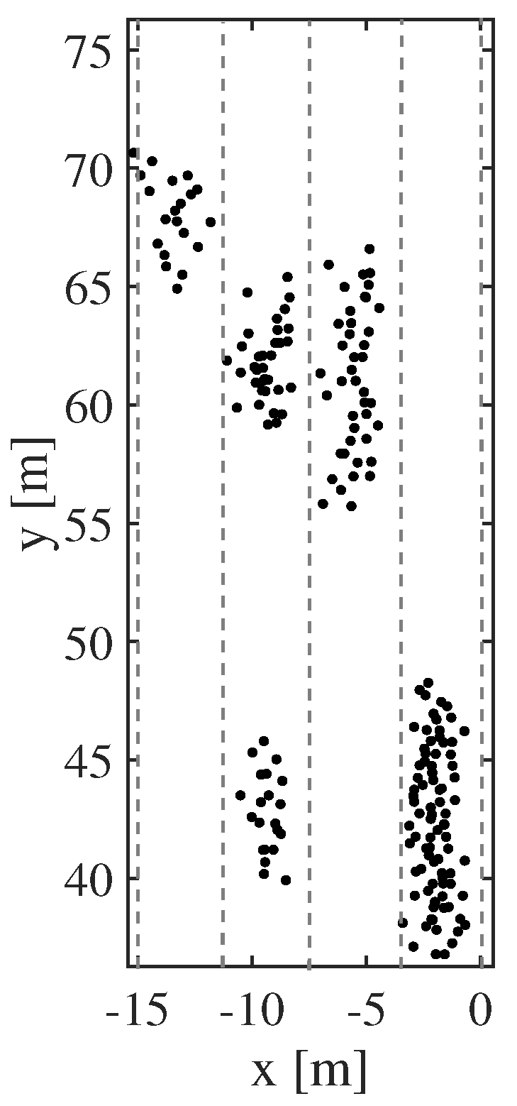
Scene 3: There are five vehicles with a relatively short driving distance on the straight four-lane highway. There are many vehicles blocking each other, as shown in Figure 13. At this point, the radar returns a total of 202 valid sampling points, and their distribution is shown in Figure 14.
The comparison of clustering results of various algorithms in this scene is shown in Figure 15.
In this scene, the number of adjacent vehicles is relatively large, and several vehicles are covering each other, resulting in uneven distribution of sampling points and fewer sampling points for small cars. The DBSCAN algorithm classifies by density and results in a large number of clusters. The iterative update of the fuzzy matrix and the cluster center point by the FCM algorithm cannot solve the problem of distinguishing adjacent targets well. The K-Means algorithm does not classify well for adjacent sample points. The clustering results obtained by the density peak fuzzy clustering algorithm in this paper can correspond well to the real scene. Compared with the results of other algorithms, the conclusion of the new algorithm is better.
Next, in order to compare the clustering accuracy of each algorithm, the accuracy of the clustering is defined as:
R a t e = K N × 100 % ,
where R a t e represents the clustering accuracy rate; K represents the number of sampling points for correct clustering; N represents the total number of sample points participating in the classification. The accuracy comparison of each algorithm is shown in Figure 16.
It can be seen from the figure that, for the three practical experimental scenes in this paper, the SDPFC algorithm proposed in this paper has the best results, and the average accuracy can reach more than 95%.
In order to present the clustering results of the SDPFC algorithm better, in addition to the above three classic scenes, four scenes with adjacent vehicles are selected. The real situation of the four scenes are shown in Figure 17. In addition, the clustering results of the SDPFC algorithm are shown in Figure 18.
In order to visually compare the real-time performance of each algorithm, this paper selects ten different traffic scenes and performs the same experiments on the four algorithms mentioned in this paper to verify the real-time performance of the algorithm. Select all sampling points in about 0.2 s as the input data for the experiment in each scene.
As can be seen from Table 1, the SDPFC algorithm proposed in this paper is the fastest of the four algorithms, and it is about 2.04 times faster than the slowest algorithm. The K-Means algorithm is ranked second because of its simple calculation method. The slowest running speed is the FCM algorithm, mainly because of the uncertainty of the initial point in the FCM algorithm, resulting in the number of iterative updates that have been maintained at a high level.
After comparing the clustering accuracy and running speed of each algorithm in a certain scene, this paper presents statistical images of the average of the accuracy of various algorithms in several specific scenes. The purpose is to show the stability of the clustering of these algorithms in the given scene. It can be seen from Figure 19 that the SDPFC algorithm proposed in this paper has good adaptability in a certain scene and can maintain high accuracy. In addition, the K-Means algorithm is more adaptable, but the accuracy is not high. The adaptability of DBSCAN and FCM is relatively poor, but the accuracy of DBSCAN is significantly higher than that of FCM.
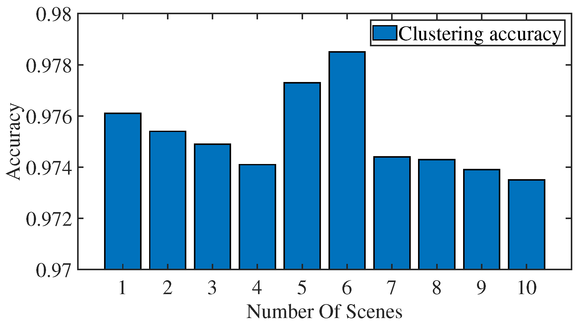
In order to show the clustering results of the SDPFC algorithm better, a new experiment is performed. Statistics on the accuracy of clustering adjacent vehicles in 1000 scenes. A vehicle sampling point collected every 40 milliseconds is defined as a scene. In each scene, there are 2–5 passing vehicles, and the radar echo signals are processed to obtain 100–300 sampling points. Comparing each scene with the real image and the clustering result graph, calculate the clustering accuracy according to the concept proposed by Formula (38). The specific experimental results are shown in Figure 20, where 1 on the abscissa represents the average clustering accuracy of the scene 1 to the scene 100, 2 represents the average clustering accuracy of the scene 101 to the scene 200, and so on. Finally, according to statistics, 3627 passing vehicles are processed in 1000 scenes, of which 3537 obtained correct clustering results. The correct clustering rate is about 97.52%.
Through the experiments in this section, we can conclude that: under the real highway traffic scene given in this paper, the SDPFC algorithm proposed in this paper can solve the problem of inaccurate clustering results of adjacent vehicles. The algorithm can complete the operation in a short time while maintaining high accuracy and has strong adaptability to scene changes.

6. Conclusions

This paper proposes a new quadratic modified clustering algorithm called a Spindle-based Density Peak Fuzzy Clustering (SDPFC) algorithm, which has several new features. After analyzing the characteristics of the radar sampling points of the vehicles in the experimental scene, it was found that each sampling point cluster of the vehicle would have a density peak. Using this feature, the initial clustering algorithm based on density peak is first used to obtain the number of clusters, that is, the number of vehicles and the cluster center of each cluster. Next, using the two important pieces of information just obtained, the clustering result of the first step is corrected by the iterative updating method of the fuzzy matrix and the spindle, and then the final clustering result is obtained. In this paper, experimental data are collected from real highway scenes. Three typical experimental scenes are listed in the paper. The experimental results show that the proposed algorithm can solve the clustering problem of adjacent vehicles and covered vehicles in some specific scenes of the highway. The algorithm has high accuracy, high real-time, and strong robustness.

Author Contributions

Conceptualization, methodology, formal analysis, project administration and funding acquisition, L.C.; investigation, validation, visualization, software, and writing—original draft, Y.L.; resources and data curation, D.W.; supervision, validation, writing—review and editing, T.W.; writing—review and editing, C.F. All authors have read and agreed to the published version of the manuscript.

Funding

This research was funded by the National Natural Science Foundation of China under Grant No. 61671069 and by Qin Xin Talents Cultivation Program under Grant No. QXTCP A201902.

Acknowledgments

This work is partially supported by the National Natural Science Foundation of China under Grant No. 61671069 and by Qin Xin Talents Cultivation Program under Grant No. QXTCP A201902.

Conflicts of Interest

The authors declare no conflict of interest. The funders had no role in the design of the study; in the collection, analyses, or interpretation of data; in the writing of the manuscript, or in the decision to publish the results.

Appendix A

Appendix A.1.

Proposition A1.
Formula (25) is continuously differentiable function.
Proof. 
Taking cluster 1 as an example, if Formula (25) is a continuously differentiable function, then the existence of the result of Formula (A1) needs to be proven:
lim Δ B i j 0 Δ T Δ B i j = lim Δ B i j 0 f B 1 j + Δ B i j f B 1 j Δ B i j .
Substituting Formula (25) into Formula (A1) gives:
lim Δ B i j 0 i = 1 I j = 1 k B 1 j + Δ B i j m D j ( i ) 2 i = 1 I j = 1 k B 1 j m D j ( i ) 2 Δ B i j .
Expanding Formula (A2) gives:
lim Δ B i j 0 i = 1 I j = 1 k B 1 j m + C m 1 B 1 j m 1 Δ B i j + + C m q B 1 j m q Δ B i j q + + Δ B i j m D j ( i ) 2 Δ B i j lim Δ B i j 0 i = 1 I j = 1 k B 1 j m D j ( i ) 2 Δ B i j .
Simplifying Formula (A3) gives:
lim Δ B i j 0 i = 1 I j = 1 k C m 1 B 1 j m 1 D j ( i ) 2 + + i = 1 I j = 1 k C m q B 1 j m q D j ( i ) 2 Δ B i j q 1 + + i = 1 I j = 1 k Δ B i j m 1 D j ( i ) 2 .
It is finally calculated by Formula (A1):
lim Δ B i j 0 Δ T Δ B i j = i = 1 I j = 1 k C m 1 B 1 j m 1 D j ( i ) 2 .
As can be seen from the expression of Formula (A5), in cluster 1, lim Δ B i j 0 Δ T Δ B i j exists, thus proving that Formula (25) is continuously differentiable. □

References

  1. Virant, M.; Ambro, M. Universal Safety Distance Alert Device for Road Vehicles. Electronics 2016, 5, 19. [Google Scholar] [CrossRef] [Green Version]
  2. Toker, O.; Brinkmann, M. A Novel Nonlinearity Correction Algorithm for FMCW Radar Systems for Optimal Range Accuracy and Improved Multitarget Detection Capability. Electronics 2019, 8, 1290. [Google Scholar] [CrossRef] [Green Version]
  3. Su, Y.; Guo, Z.; Zhang, Q. An Improved Intelligent Transportation Algorithm Based on Image Processing. In Proceedings of the 2018 8th International Conference on Intelligent Systems, Modelling and Simulation (ISMS), Kuala Lumpur, Malaysia, 8–10 May 2018; pp. 22–25. [Google Scholar]
  4. Hu, R.; Peng, Z.; Ma, J. A Vehicle Target Recognition Algorithm for Wide-Angle SAR Based on Joint Feature Set Matching. Electronics 2019, 8, 1252. [Google Scholar] [CrossRef] [Green Version]
  5. Kim, Y.D.; Son, G.J.; Song, C.H.; Kim, H.K. On the Deployment and Noise Filtering of Vehicular Radar Application for Detection Enhancement in Roads and Tunnels. Sensors 2018, 18, 837. [Google Scholar]
  6. Zhai, G.; Wu, C.; Wang, Y. Millimeter Wave Radar Target Tracking Based on Adaptive Kalman Filter. In Proceedings of the 2018 IEEE Intelligent Vehicles Symposium (IV), Changshu, Suzhou, China, 26–30 June 2018; pp. 453–458. [Google Scholar]
  7. Felguera-Martin, D.; Gonzalez-Partida, J.; Almorox-Gonzalez, P.; Burgos-Garcĺa, M. Vehicular Traffic Surveillance and Road Lane Detection Using Radar Interferometry. IEEE Trans. Veh. Technol. 2012, 61, 959–970. [Google Scholar] [CrossRef] [Green Version]
  8. He, X.; Wang, T.; Liu, W.; Luo, T. Measurement Data Fusion Based on Optimized Weighted Least-Squares Algorithm for Multi-Target Tracking. IEEE Access 2019, 7, 13901–13916. [Google Scholar] [CrossRef]
  9. Behrendt, R. Traffic monitoring radar for road map calculation. In Proceedings of the 2016 17th International Radar Symposium (IRS), Krakow, Poland, 10–12 May 2016; pp. 1–4. [Google Scholar]
  10. Meshram, S.A.; Lande, R.S. Traffic surveillance by using image processing. In Proceedings of the 2018 International Conference on Research in Intelligent and Computing in Engineering (RICE), San Salvador, El Salvador, 22–24 August 2018; pp. 1–3. [Google Scholar]
  11. Ozatay, E.; Ozguner, U.; Filev, D.; Michelini, J. Bayesian Traffic Light Parameter Tracking Based on Semi-Hidden Markov Models. IEEE Trans. Intell. Transp. Syst. 2016, 17, 2998–3008. [Google Scholar] [CrossRef]
  12. Wang, X.; Hua, X.; Xiao, F.; Li, Y.; Hu, X.; Sun, P. Multi-Object Detection in Traffic Scenes Based on Improved SSD. Electronics 2018, 7, 302. [Google Scholar] [CrossRef] [Green Version]
  13. Wu, B.; Feng, Y.P.; Zheng, H.Y.; Chen, X. Dynamic Cluster Members Scheduling for Target Tracking in Sensor Networks. IEEE Sens. J. 2016, 16, 7242–7249. [Google Scholar] [CrossRef]
  14. Wang, T.; Wang, X.; Shi, W.; He, Z.; Zhao, Z.; Tongsheng, X. Target Localization and Tracking Based on Improved Bayesian Enhanced Least-Squares Algorithm in Wireless Sensor Networks. Comput. Netw. 2019, 167, 106968. [Google Scholar] [CrossRef]
  15. Wang, X.; Wang, T.; Chen, S.; Fan, R.; Xu, Y.; Wang, W.; Li, H.; Xia, T. Track fusion based on threshold factor classification algorithm in wireless sensor networks. Int. J. Commun. Syst. 2016, 30, 1–15. [Google Scholar] [CrossRef]
  16. Janda, F.; Pangerl, S.; Schindler, A. A road edge detection approach for marked and unmarked lanes based on video and radar. In Proceedings of the 16th International Conference on Information Fusion, Istanbul, Turkey, 9–12 July 2013. [Google Scholar]
  17. Wang, T.; Wang, X.; Zhao, Z.; He, Z.; Xia, T. Measurement Data Classification Optimization Based on a Novel Evolutionary Kernel Clustering Algorithm for Multi-target Tracking. IEEE Sens. J. 2018, 18, 3722–3733. [Google Scholar] [CrossRef]
  18. Gan, G.; Ng, K.P. k-means clustering with outlier removal. Pattern Recognit. Lett. 2017, 90, 8–14. [Google Scholar] [CrossRef]
  19. Na, S.; Xumin, L.; Yong, G. Research on k-means Clustering Algorithm: An Improved k-means Clustering Algorithm. In Proceedings of the 2010 Third International Symposium on Intelligent Information Technology and Security Informatics, Jinggangshan, China, 2–4 April 2010; pp. 63–67. [Google Scholar]
  20. Lai, Y.; He, S.; Lin, Z.; Yang, F.; Zhou, Q.; Zhou, X. An Adaptive Robust Semi-supervised Clustering Framework Using Weighted Consensus of Random k-Means Ensemble. IEEE Trans. Knowl. Data Eng. 2019. [Google Scholar] [CrossRef]
  21. Jiang, Z.; Li, T.; Min, W.; Qi, Z.; Rao, Y. Fuzzy c-means clustering based on weights and gene expression programming. Pattern Recognit. Lett. 2017, 90, 1–7. [Google Scholar] [CrossRef]
  22. Abdullatif, A.; Masulli, F.; Rovetta, S. Clustering of nonstationary data streams: A survey of fuzzy partitional methods. WIREs Data Min. Knowl. Discov. 2018, 8, e1258. [Google Scholar] [CrossRef] [Green Version]
  23. Pedrycz, W.; Waletzky, J. Fuzzy clustering with partial supervision. IEEE Trans. Syst. Man Cybern. Part B (Cybernetics) 1997, 27, 787–795. [Google Scholar] [CrossRef] [Green Version]
  24. Yang, T.; Lee, C.; Yen, S. Fuzzy objective functions for robust pattern recognition. In Proceedings of the 2009 IEEE International Conference on Fuzzy Systems, Jeju Island, Korea, 20–24 August 2009; pp. 2057–2062. [Google Scholar]
  25. Lin, K.P. A Novel Evolutionary Kernel Intuitionistic Fuzzy C -means Clustering Algorithm. IEEE Trans. Fuzzy Syst. 2014, 22, 1074–1087. [Google Scholar] [CrossRef]
  26. Casalino, G.; Castellano, G.; Mencar, C. Data Stream Classification by Dynamic Incremental Semi-Supervised Fuzzy Clustering. WIREs Data Min. Knowl. Discov. 2019, 28, 1960009. [Google Scholar] [CrossRef]
  27. Liu, B. A Fast Density-Based Clustering Algorithm for Large Databases. In Proceedings of the 2006 International Conference on Machine Learning and Cybernetics, Dalian, China, 13–16 August 2006; pp. 996–1000. [Google Scholar]
  28. Hiep, N.H. Privacy-Preserving Mechanisms for k-Modes Clustering. Comput. Secur. 2018, 78, 60–75. [Google Scholar]
  29. Kanika; Rani, K.; Sangeeta; Preeti. Visual Analytics for Comparing the Impact of Outliers in k-Means and k-Medoids Algorithm. In Proceedings of the 2019 Amity International Conference on Artificial Intelligence (AICAI), Dubai, United Arab Emirates, 4–6 February 2019; pp. 93–97. [Google Scholar]
  30. Wang, J.; Wang, K.; Niu, J.; Liu, W. A K-medoids based clustering algorithm for wireless sensor networks. In Proceedings of the 2018 International Workshop on Advanced Image Technology (IWAIT), Chiang Mai, Thailand, 7–9 January 2018; pp. 1–4. [Google Scholar]
  31. Hathaway, R.J.; Bezdek, J.C. Fuzzy c-means clustering of incomplete data. IEEE Trans. Syst. Man Cybern. Part B (Cybernetics) 2001, 31, 735–744. [Google Scholar] [CrossRef] [Green Version]
  32. Trisminingsih, R.; Shaztika, S.S. ST-DBSCAN clustering module in SpagoBI for hotspots distribution in Indonesia. In Proceedings of the 2016 3rd International Conference on Information Technology, Computer, and Electrical Engineering (ICITACEE), Semarang, Indonesia, 19–20 October 2016; pp. 327–330. [Google Scholar]
  33. Rodriguez, A.; Laio, A. Clustering by fast search and find of density peaks. Science 2014, 344, 1492–1496. [Google Scholar] [CrossRef] [PubMed] [Green Version]
  34. Zhou, H.; Liu, Q.; Chen, D.; Chen, W.; Shen, F. Doppler Shift and Height Detection of Obstacle Based on FMCW Radar Sensor. In Proceedings of the 2015 International Conference on Cyber-Enabled Distributed Computing and Knowledge Discovery, Xi’an, China, 17–19 September 2015; pp. 399–402. [Google Scholar]
  35. Carli, R.; Dotoli, M.; Epicoco, N.; Angelico, B.; Vinciullo, A. Automated evaluation of urban traffic congestion using bus as a probe. In Proceedings of the 2015 IEEE International Conference on Automation Science and Engineering (CASE), Gothenburg, Sweden, 24–28 August 2015; pp. 967–972. [Google Scholar] [CrossRef]
  36. Li, M.; Meng, D.; Gu, S.; Liu, S. Research and Improvement of DBSCAN Cluster Algorithm. In Proceedings of the 2015 7th International Conference on Information Technology in Medicine and Education (ITME), Huangshan, China, 13–15 November 2015; pp. 537–540. [Google Scholar]
  37. Sharma, S.; Sharma, A.K.; Soni, D. Enhancing DBSCAN algorithm for data mining. In Proceedings of the 2017 International Conference on Energy, Communication, Data Analytics and Soft Computing (ICECDS), Chennai, India, 1–2 August 2017; pp. 1634–1638. [Google Scholar]
  38. Dong, G.; Jin, Y.; Wang, S.; Li, W.; Tao, Z.; Guo, S. DB-Kmeans: An Intrusion Detection Algorithm Based on DBSCAN and K-means. In Proceedings of the 2019 20th Asia-Pacific Network Operations and Management Symposium (APNOMS), Matsue, Japan, 18–20 September 2019; pp. 1–4. [Google Scholar]
  39. Nazari, M.; Shanbehzadeh, J.; Sarrafzadeh, A. Fuzzy C-means based on Automated Variable Feature Weighting. Lect. Notes Eng. Comput. Sci. 2013, 2202, 25–29. [Google Scholar]
  40. Zhang, L.; Pedrycz, W.; Lu, W.; Liu, X.; Zhang, L. An interval weighed fuzzy c-means clustering by genetically guided alternating optimization. Expert Syst. Appl. 2014, 41, 5960–5971. [Google Scholar] [CrossRef]
  41. Pedrycz, W.; Waletzky, J. Fuzzy clustering with semantic interpretation. Appl. Soft Comput. 2015, 26, 21–30. [Google Scholar] [CrossRef]
  42. Cao, J.; Zhong, C.; Li, D. Incomplete data fuzzy C-means method based on spatial distance of sample. In Proceedings of the 2019 Chinese Control Conference (CCC), Guangzhou, China, 27–30 July 2019; pp. 7618–7622. [Google Scholar]
  43. Wu, H.; Pang, B.; Dai, D.; Wu, J.; Wang, X. Unmanned Aerial Vehicle Recognition Based on Clustering by Fast Search and Find of Density Peaks (CFSFDP) with Polarimetric Decomposition. Electronics 2018, 7, 364. [Google Scholar] [CrossRef] [Green Version]
  44. Cao, S.; Wang, S.; Zhang, Y. Density-Based Fuzzy C-Means Multi-center Re-clustering Radar Signal Sorting Algorithm. In Proceedings of the 2018 17th IEEE International Conference on Machine Learning and Applications (ICMLA), Orlando, FL, USA, 17–20 December 2018; pp. 891–896. [Google Scholar]
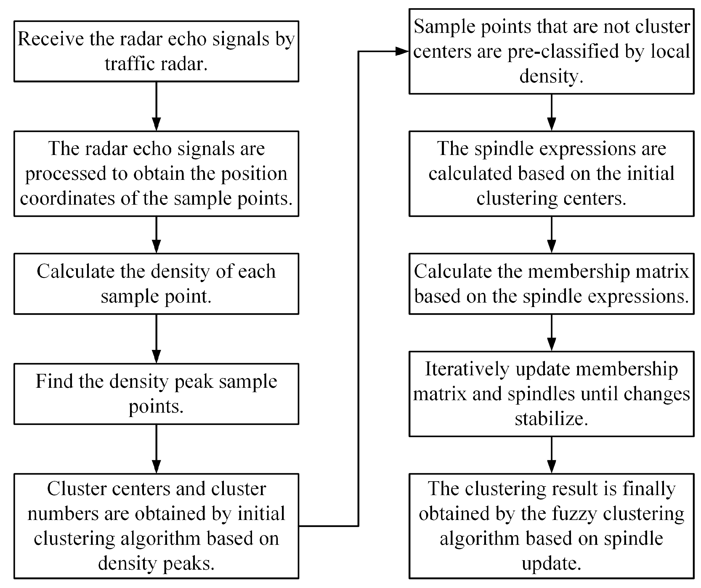
Figure 1. The main diagram of the system.
Electronics 09 00046 g001
Figure 2. Real traffic scene.
Electronics 09 00046 g002
Figure 3. Decision graph.
Electronics 09 00046 g003
Figure 4. Initial clustering result.
Electronics 09 00046 g004
Figure 5. The SDPFC algorithm final clustering result.
Electronics 09 00046 g005
Figure 6. The experimental scene and the placement of the radar.
Electronics 09 00046 g006
Figure 7. The real situation of Scene 1.
Electronics 09 00046 g007
Figure 8. Sampling points of Scene 1.
Electronics 09 00046 g008
Figure 9. The clustering results of each algorithm: (a) DBSCAN; (b) FCM; (c) K-Means; and (d) SDPFC.
Electronics 09 00046 g009
Figure 10. The real situation of Scene 2.
Electronics 09 00046 g010
Figure 11. Sampling points of Scene 2.
Electronics 09 00046 g011
Figure 12. The clustering results of each algorithm: (a) DBSCAN; (b) FCM; (c) K-Means; and (d) SDPFC.
Electronics 09 00046 g012
Figure 13. The real situation of Scene 3.
Electronics 09 00046 g013
Figure 14. Sampling points of Scene 3.
Electronics 09 00046 g014
Figure 15. The clustering results of each algorithm: (a) DBSCAN; (b) FCM; (c) K-Means; and (d) SDPFC.
Electronics 09 00046 g015
Figure 16. Clustering accuracy histogram.
Electronics 09 00046 g016
Figure 17. The real situation of the four scenes: (a) Scene4; (b) Scene5; (c) Scene6; and (d) Scene7.
Electronics 09 00046 g017
Figure 18. The clustering results of each scene: (a) Scene4; (b) Scene5; (c) Scene6; and (d) Scene7.
Electronics 09 00046 g018
Figure 19. Comparison of stability of each algorithm.
Electronics 09 00046 g019
Figure 20. Accuracy of clustering using SDPFC algorithm in 1000 scenes.
Electronics 09 00046 g020
Table 1. Time-consuming table for each algorithm.
Time Consuming/sAlgorithms
Experiment NumberDBSCANFCMK-MeansSDPFC
10.01390.03580.02700.0330
20.01280.03180.02960.0298
30.01410.03370.02620.0322
40.01380.03250.02650.0351
50.01290.03580.02540.0325
60.01320.03340.02590.0329
70.01350.03150.02490.0332
80.01390.03240.02660.0336
90.01340.03490.02710.0332
100.01360.03380.02560.0319
Average time consumption/s0.01350.03360.02660.0327