Nonsmooth Current-Constrained Control for a DC–DC Synchronous Buck Converter with Disturbances via Finite-Time-Convergent Extended State Observers

Abstract

This study investigates the problem of overlarge current protection for a DC–DC synchronous buck converter with the existence of uncertainties and disturbances. Aiming to deal with the hardware damage in the electric circuit of a DC–DC buck that may be caused by overlarge transient current, a new nonsmooth current-constrained control (NCC) algorithm is proposed to replace the traditional ones, which use conservative coefficients to satisfy current constraint, leading to a sacrifice of dynamic performance. Based on the homogeneous system technique, a nonsmooth state feedback controller is improved by adding a penalty term that prompts the adaptive gain of the controller according to the inductor current and current constraint. Then by using two finite-time extended state observers (FTESO), the unmatched disturbances and matched disturbances can be compensated to enhance the robustness of the DC–DC synchronous buck converter. The effect of proposed scheme has been verified by experimental results.

1. Introduction

Distributed power supply systems are widely used in aerospace, marine, communications, and other fields, the system only provides power bus, and the power supply inside the equipment is solved by their own power converters to improve the stability of the system and facilitate the maintenance of the system. As a kind of energy conversion device from DC to DC, a DC–DC converter has a simple structure, capable of realizing high efficiency power conversion and being modularized. DC–DC converters are widely used in power supply and load in this kind of power supply system structure [1,2].

A DC–DC converter is a kind of variable structure system with switching devices [3]. The circuit often contains capacitors, inductances and other energy storage elements, and their charging and discharging behavior has the characteristics of time-varying nonlinearity. In addition, the modeling process is too idealized, and some unmodeled dynamics are often neglected. These unmodeled dynamic characteristics are usually generated by sensors, actuators, and so on. Therefore, it is necessary to study the influence of unmodeled dynamics on a DC converter system. With the shortage of fossil energy, renewable energy technologies, such as wind energy and solar energy, have developed rapidly, and the capacity of distributed renewable energy generation systems have been increasing. However, there are many characteristics such as unpredictability, intermittency, and non-dispatch in such renewable energy systems. At the same time, there are a large number of non-linear and time-varying loads in the system. Due to these factors, input voltage and load resistance are uncertain, which affects the output accuracy of the power converter [4,5]. Therefore, in the case of strong disturbance and parameter uncertainties, the design of a robust controller [6,7,8] with high accuracy has become a research hotspot.

Due to the characteristics of DC–DC circuit and many situations in practical application, which means adapting the control law for these switched systems is needed [9,10]. Pulse width modulation technology based on linear control theory cannot meet the requirements in transient characteristics and robustness. Many scholars have attempted to improve the performance of power converters by using non-linear control methods. At present, for the control of power electronic converters, common non-linear control methods include Bang-Bang control [11,12], sliding mode variable structure control [13,14], fuzzy control [15,16], finite time control [2,3,17], and so on.

Nonlinear control algorithms such as Bang-Bang control, sliding mode variable structure control, and fuzzy control can only theoretically guarantee the asymptotic stability of the control system. In practical application, convergence performance is a key index. However, according to this kind of control design method, the fastest convergence speed of a closed-loop system can only be in exponential form, so these control methods belong to the solution of infinite-time stability problem [17,18]. Therefore, finite-time control is proposed. Theoretical analysis shows that when there are no external disturbances, this method can make the system state meet the required target state in finite time. Considering that disturbances are inevitable in practice, the closed-loop system still has better accuracy, robustness, and disturbances rejection performance because of the existence of fractional power term [19,20].

It should be pointed out, that a DC–DC converter requires higher and higher voltage response speed, resulting in a large overshoot of inductance current in the circuit when the converter starts [21]. If there are no restrictions, it is easy to damage the circuit hardware, especially for high-power converters. One way to solve this problem is to add a current limiter to the hardware circuit to protect the circuit. However, the cost of adding this protection circuit increases and the efficiency of energy conversion decreases [22,23]. In [21], it is pointed out that another method is to consider current constraints when designing the digital controllers of buck circuits to avoid additional burdens on hardware circuits. In traditional control methods, conservative control parameters can be selected to meet current constraints in controller design. For example, in proportion integration differentiation (PID) control, measures to reduce proportional gain can be taken. However, such methods sacrifice the dynamic characteristics of the system, which runs counter to the requirement of improving system response. In recent years, the addition of a penalty mechanism in controls as an effective method to solve the constraints in the system has been gradually developed. Model predictive control (MPC) is one of the typical application modes. By making full use of future information, MPC transforms control problems into optimization problems, so as to "actively" deal with constraints [24,25], i.e., to anticipate the possibility of exceeding constraints in the future, and take necessary control actions in advance to make it no longer happen [26]. In [27], a computationally friendly sub-optimal nonlinear model predictive control (NMPC) algorithm based on infinity norm-based artificial Lyapunov function with prior input-to-state stabilizing (ISS) guarantee is applied to the real-time control of buck DC–DC power converter, which satisfies the limitation of inductance current. However, when MPC is adversely affected by uncertainties and disturbances in the circuit model, its feedback regulation mode is relatively slow [28]. In addition, MPC has a large number of computations due to the existence of optimization problems, which put forward higher requirements for hardware. In addition, another application is to use the barrier function when designing the Lyapunov function in the backstepping control algorithm [29,30]. This method needs to use the barrier Lyapunov function for the constrained state variables in the recursive design process of backstepping control, but it also leads to the constraints of the virtual controller in the design process [23].

Considering the matched and unmatched disturbances in DC–DC converters, disturbance observers are needed to meet the control requirements. Extended state observers (ESO) are widely used because they require little information for dynamic systems and can estimate unmodeled dynamics, uncertainties, and external disturbances online [31]. A traditional ESO can only satisfy the requirement of asymptotic stability. Therefore, the ESO needs to be designed based on finite-time stability theory to achieve faster convergence rate and higher estimation accuracy.

This paper takes the common DC–DC synchronous buck converter in a DC distributed power supply system as an example. Based on the homogeneous system technique, a nonsmooth algorithm has been designed to achieve better convergence characteristics of the DC–DC synchronous buck converter system. At the same time, a simple way to satisfy the current constraint is proposed by using barrier Lyapunonv function (BLF). To counteract the matched/unmatched disturbances, two finite-time extended state observers (FTESOs) are used which can guarantee fast convergence rate and robustness of the converter system via the super-twisting algorithm

2. Model Description and Problem Formulation

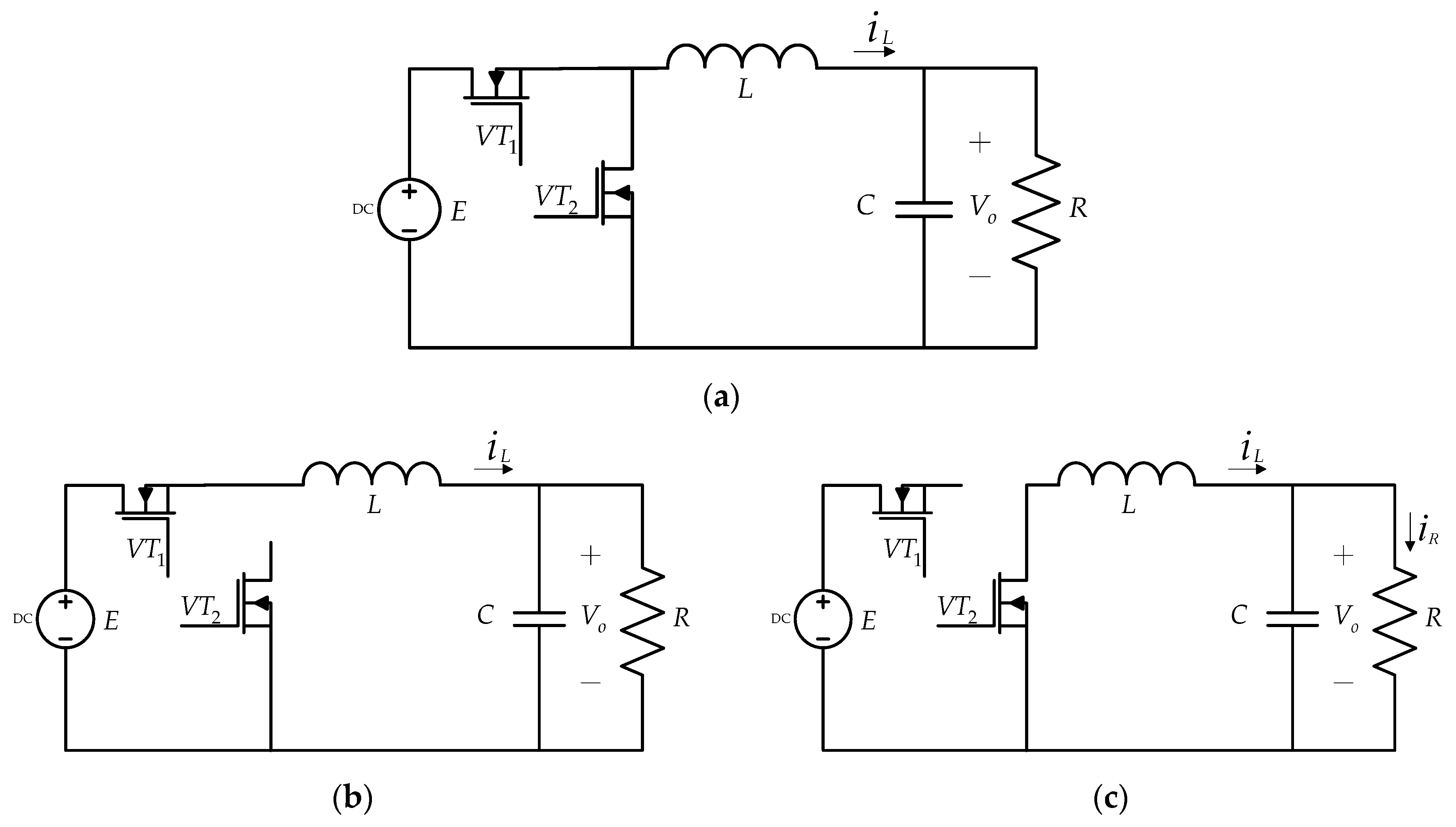
2.1. Modeling the DC–DC Synchronous Buck Converter

The circuit topology of the DC-DC buck converter using synchronous rectification technology is shown in Figure 1, where E is the input DC voltage source, $V{T}_1$ and $V{T}_2$ are the controllable switches ($V{T}_1$ is the main switch and $V{T}_2$ is the synchronous rectifier), $u\in [0,1]$ is the duty ratio of pulse width modulation (PWM) as the control signal, $V_o$ is the output voltage, $i_L$ is the inductance current, $i_R$ is the load current, L is the filter inductor, C is the filter capacitor, and R is the load resistance. Firstly, for the buck converter with $V{T}_1$ switching on and off, the corresponding operating modes $u=1$ and $u=0$ respectively.

When the main switch $V{T}_1$ is on and the synchronous rectifier $V{T}_2$ is off, that is, $u=1$.

$$\{\begin{array}{c}\frac{d{i}_L}{dt}=\frac{1}{L}\left(E-V_o\right)\\ \frac{d{V}_o}{dt}=\frac{1}{C}\left(i_L-\frac{V_o}{R}\right)\end{array}.$$

(1)

When the main switch $V{T}_1$ is off and the synchronous rectifier $V{T}_2$ is on, that is, $u=0$.

$$\{\begin{array}{c}\frac{d{i}_L}{dt}=-\frac{1}{L}{V}_o\\ \frac{d{V}_o}{dt}=\frac{1}{C}\left(i_L-\frac{V_o}{R}\right)\end{array}.$$

(2)

Combining Equations (1) and (2), the differential equation model of synchronous buck converter under two working modes of $u=1$ and $u=0$ is:

$$\{\begin{array}{c}\frac{d{i}_L}{dt}=\frac{1}{L}\left(uE-V_o\right)\\ \frac{d{V}_o}{dt}=\frac{1}{C}\left(i_L-\frac{V_o}{R}\right)\end{array}.$$

(3)

The above formulas use the state space averaging method, that is to say, the final state space averaging model (Equation (3)) is obtained by averaging $u=1$ and $u=0$ modes over one cycle, in which $V_o$ and $i_L$ are the average values of output voltage and inductance current over a switching period [20].

2.2. Problem formulation

Let $x_1=V_o-V_r$, $x_2={\dot{V}}_o$, where $V_r$ is the desired output voltage. Consider the disturbances caused by the change of load resistance and input voltage in synchronous buck converter and the uncertainties of inductance and capacitance parameters, the converter system (Equation (3)) can be rewritten as follows

$$\{\begin{array}{c}{\dot{x}}_1=x_2={\overline{x}}_2+d_1\\ {\dot{x}}_2=\frac{u{E}_0-V_r}{L_0{C}_0}-\frac{x_1}{L_0{C}_0}-\frac{x_2}{R_0{C}_0}+d_2\end{array},$$

(4)

where ${\overline{x}}_2$, $d_1$, and $d_2$ are denoted by

$${\overline{x}}_2=\frac{1}{C_0}\left(i_L-\frac{V_o}{R_0}\right),$$

(5)

$$d_1=\left(\frac{1}{C}-\frac{1}{C_0}\right)i_L-\left(\frac{1}{RC}-\frac{1}{R_0{C}_0}\right)V_o,$$

(6)

$$d_2=\left(\frac{E}{LC}-\frac{E_0}{L_0{C}_0}\right)u-\left(\frac{1}{LC}-\frac{1}{L_0{C}_0}\right)V_o-\left(\frac{1}{RC}-\frac{1}{R_0{C}_0}\right)\left(\frac{i_L}{C_0}-\frac{V_o}{R_0{C}_0}+d_1\right),$$

(7)

and $R_0$, $C_0$, $E_0$, and $L_0$ denote the nominal values of $R$, $C$, $E$, and $L$ respectively.

3. Controller Design

Definition 1.

In this article, for the convenience of writing, the following simplifications are utilized

$$\lceil x{\rfloor }^{\alpha }={\left|x\right|}^{\alpha }sign\left(x\right),$$

(8)

where $\alpha \in \mathrm{R}$, and $sign(\ast )$ is a standard sign function.

Since both matched and mismatched disturbances can lead to the decrease of the static accuracy, the first step in the design of the controller was to estimate the matched and mismatched disturbances by using two FTESOs. Secondly, a simple nonsmooth current-constrained controller based on homogeneous system theory was designed to make the output voltage follow the reference value. The control structure is shown in Figure 2.

3.1. Finite-Time Extended State Observer Design

Assumption 1

[32]. Suppose that the unknown lumped disturbances which can be describe as Equations (6) and (7) are continuously differentiable with respect to time.

Let $z_{11}$, $z_{21}$ denote the state variable $x_1$, $x_2$ and introduce the extended state variable $z_{12}$, $z_{22}$ denotes the lumped disturbance $d_1$, $d_2$ with ${\dot{z}}_{i2}=g_i\left(t\right)$, $i=1,2$. For the lumped disturbances in DC–DC synchronous buck dynamic model (Equation (4)), the FTESO proposed in [32] can be designed as follows

$$\{\begin{array}{c}{e}_{11}=z_{11}-{\widehat{z}}_{11}\\ {\dot{\widehat{z}}}_{11}={\overline{x}}_2+{\widehat{z}}_{12}+{\beta }_{11}\left(\lceil e_{11}\rfloor {}^{\frac{1}{2}}+e_{11}\right)\\ {\dot{\widehat{z}}}_{12}={\beta }_{12}\left(\frac{1}{2}sign\left(e_{11}\right)+\frac{3}{2}\lceil e_{11}\rfloor {}^{\frac{1}{2}}+e_{11}\right)\end{array},$$

(9)

$$\{\begin{array}{c}{e}_{21}=z_{21}-{\widehat{z}}_{21}\\ {\dot{\widehat{z}}}_{21}=\frac{u{E}_0-V_r}{L_0{C}_0}-\frac{x_1}{L_0{C}_0}-\frac{x_2}{R_0{C}_0}+{\widehat{z}}_{22}+{\beta }_{21}\left(\lceil e_{21}\rfloor {}^{\frac{1}{2}}+e_{21}\right)\\ {\dot{\widehat{z}}}_{22}={\beta }_{22}\left(\frac{1}{2}sign\left(e_{21}\right)+\frac{3}{2}\lceil e_{21}\rfloor {}^{\frac{1}{2}}+e_{21}\right)\end{array},$$

(10)

where ${\widehat{z}}_{ij}$ is the estimation of the variables $z_{ij}$, ${\beta }_{ij}>0$ is the gain of FTESO to be tuned, $\left(i,j=1,2\right)$.

Assumption 2

[32,33]. The derivative of the extended state variable is unknown but bounded, i.e., existing a positive constant $\overline{g}$ such that $\Vert g_i\left(t\right)\Vert \le \overline{g}$, $i=1,2$.

By defining the observation error of the lumped disturbance as $e_{i2}=z_{i2}-{\widehat{z}}_{i2}$, $\left(i,j=1,2\right)$ and combining with Equations (8) and (9), we can obtain the following dynamic error equation

$$\{\begin{array}{c}{\dot{e}}_{i1}=e_{i2}-{\beta }_{i1}\left(\lceil e_{i1}\rfloor {}^{\frac{1}{2}}+e_{i1}\right)\\ {\dot{e}}_{i2}=g_i\left(t\right)-{\beta }_{i2}\left(\frac{1}{2}sign\left(e_{i1}\right)+\frac{3}{2}\lceil e_{i1}\rfloor {}^{\frac{1}{2}}+e_{i1}\right)\end{array},i=1,2.$$

(11)

According to [32], the dynamic error states variables in Equation (10) will converge to zero in finite time under the Assumptions 1 and 2, and the estimated value ${\widehat{z}}_{ij}$ can converge to the real value $z_{ij}$ in a finite time $t_f$, $\left(i,j=1,2\right)$.

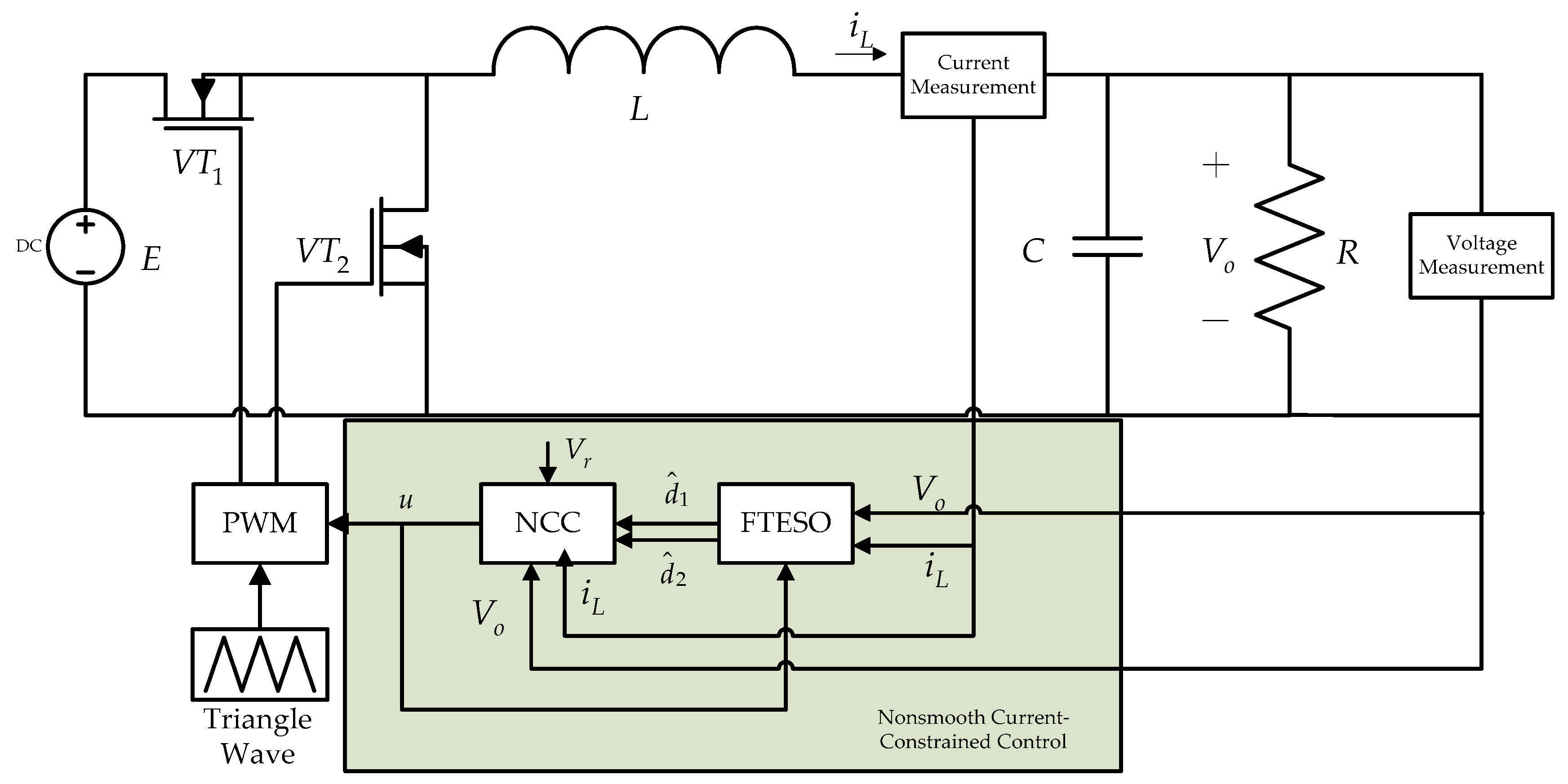
3.2. Nonsmooth Current-Constrained Control with Disturbance Compensation

Definition 2

[34]. Let $f\left(x\right)={\left(f_1\left(x\right),\cdots ,f_n\left(x\right)\right)}^T:R^n\to R^n$ be a continuous vector field. If for any given $\epsilon >0$, $x\in R^n$, there exists $\left(r_1,\cdots ,r_n\right)\in R^n$ where $r_i>0\left(i=1,\cdots ,n\right)$, such that

$$f_i\left({\epsilon }^{r_1}{x}_1,\cdots ,{\epsilon }^{r_1}{x}_n\right)={\epsilon }^{k+r_i}{f}_i\left(x\right), i=1,\cdots n,$$

(12)

then $f\left(x\right)$ is to be homogeneous of degree $k$ with respect to $\left(r_1,\cdots ,r_n\right)$, where $k>-min\left\{r_1,\cdots ,r_n\right\}$.

Definition 3

[18]. Consider the following nonlinear system

$$\dot{x}=f\left(x\right),x\in U_0\subseteq R^n,f\left(0\right)=0,$$

(13)

where $f:U_0\to R^n$ is a continuous function with respect to $x$, and $U_0$ is the open neighborhood containing the origin $x=0$. For a given $\left(r_1,\cdots ,r_n\right)$, if the vector function $f\left(x\right)$ is homogeneous, then the system (Equation (13)) is homogeneous.

Lemma 1

[35]. For the following system

$$\dot{x}=f\left(x\right)+\widehat{f}\left(x\right),x\in R^n,\widehat{f}\left(0\right)=0,$$

(14)

where $f\left(x\right)$ is a continuous vector field of homogeneous degree $k<0$ with respect to $\left(r_1,\cdots ,r_n\right)$, and $\widehat{f}\left(x\right)$ is a continuous vector field defined on $R^n$. If $x=0$ is the asymptotically stable equilibrium point of system $\dot{x}=f\left(x\right)$ and satisfies for any $\Vert x\Vert =1$, the following formula holds

$$\underset{\epsilon \to 0}{\lim }\frac{{\widehat{f}}_i\left({\epsilon }^{r_1}{x}_1,\cdots ,{\epsilon }^{r_n}{x}_n\right)}{{\epsilon }^{k+r_i}}=0,i=1,\cdots n.$$

(15)

Then, $x=0$ is a locally finite time equilibrium point of the system (14).

For DC–DC synchronous buck converter error dynamic equation (Equation (4)), a finite-time current-constrained controller based on the FTESO designed above is designed as

$$u=\frac{V_r}{E_0}-\frac{L_0{C}_0}{E_0}\left(k_1\lceil x_1\rfloor {}^{{\gamma }_1}+k_2\lceil {\overline{x}}_2+{\widehat{d}}_1\rfloor {}^{{\gamma }_2}+\frac{l}{M^2-i_L^2}\lceil {\overline{x}}_2+{\widehat{d}}_1\rfloor {}^{{\gamma }_3}+{\widehat{d}}_2\right),$$

(16)

where ${\widehat{d}}_1,{\widehat{d}}_2$ are the lumped disturbances estimated by FTESO, $M>0$ is a constant value and $0<{\gamma }_1<1,{\gamma }_2=\frac{2{\gamma }_1}{1+{\gamma }_1},{\gamma }_3>{\gamma }_2$.

Remark 1.

In this paper, considering the damage to the hardware circuit caused by current overshoot, the inductance current is limited to a certain range in the design of the controller, so that the inductance current satisfies the constraints $\left|i_L\right|\le M$. It should be noted that the selection of current constraints will affect the tracking performance of the output voltage [21], so it needs to be selected appropriately according to the actual situation.

Remark 2

[21]. Unlike the BLF design method, in the backstepping algorithm [36,37], Equation (16) is to add the BLF-based non-linear term directly to the control law. When the constrained current term $i_L$ tends to the boundary value $\pm M$, it will play a dominant role in the control law and penalizes the current, so it is also called the penalty term.

Theorem 1.

For DC-DC synchronous buck error dynamic system (Equation (4)), the designed control method (Equation (16)) can converge the output voltage to the reference set value in a finite time and satisfy the current constraint condition $\left|i_L\right|\le M$ if $i_L\left(0\right)\in \left(-M,M\right)$.

Proof. 

Define a candidate Lyapunov function for the system described by Equation (4) as

$$V_1=k_1{\displaystyle {\int }_0^{x_1}{\lceil \tau \rfloor }^{{\gamma }_1}d\tau }+\frac{1}{2L_0{C}_0}{x}_1^2+\frac{1}{2}{x}_2^2,$$

(17)

and the first derivate of Equation (17) along Equation (4) is

$${\dot{V}}_1=k_1\lceil x_1\rfloor {}^{{\gamma }_1}{x}_2+\frac{1}{L_0{C}_0}{x}_1{x}_2+x_2\left(\frac{u{E}_0-V_r}{L_0{C}_0}-\frac{x_1}{L_0{C}_0}-\frac{x_2}{R_0{C}_0}+d_2\right).$$

(18)

By substituting the controller (Equation (16)) into Equation (18), then

$${\dot{V}}_1=x_2\left(-k_2\lceil {\overline{x}}_2+{\widehat{d}}_1\rfloor {}^{{\gamma }_2}-\frac{l}{M^2-i_L^2}\lceil {\overline{x}}_2+{\widehat{d}}_1\rfloor {}^{{\gamma }_3}-\frac{x_2}{R_0{C}_0}+d_2-{\widehat{d}}_2\right).$$

(19)

Since the estimated value of the lumped disturbances ${\widehat{d}}_1,{\widehat{d}}_2$ can converge to the real values $d_1,d_2$ in a finite time $t_f$, Equation (19) can be rewritten as

$${\dot{V}}_1=x_2\left(-k_2\lceil x_2\rfloor {}^{{\gamma }_2}-\frac{l}{M^2-i_L^2}\lceil x_2\rfloor {}^{{\gamma }_3}-\frac{x_2}{R_0{C}_0}\right)=-k_2\lceil x_2\rfloor {}^{{\gamma }_2+1}-\frac{l}{M^2-i_L^2}\lceil x_2\rfloor {}^{{\gamma }_3+1}-\frac{x_2^2}{R_0{C}_0}.$$

(20)

Assume that $[0,T)$ is the maximum time region satisfying $i_L\left(t\right)\in \left(-M,M\right),t\in [0,T)$, where $T>0$. For any initial values of current and voltage $i_L\left(0\right)\in \left(-M,M\right),V_o\left(0\right)\in \left(-\infty ,\infty \right)$, it yields

$${\dot{V}}_1\le 0,t\in [0,T),$$

(21)

then

$$V_1\left(t\right)\le V_1\left(0\right),t\in [0,T).$$

(22)

This indicates that

$$\begin{array}{ll}{V}_1\left(0\right)& =k_1{\displaystyle {\int }_0^{x_1\left(0\right)}{\lceil \tau \rfloor }^{{\gamma }_1}d\tau }+\frac{1}{2L_0{C}_0}{x}_1^2\left(0\right)+\frac{1}{2}{x}_2^2\left(0\right)\\ & \ge k_1{\displaystyle {\int }_0^{x_1\left(t\right)}{\lceil \tau \rfloor }^{{\gamma }_1}d\tau }+\frac{1}{2L_0{C}_0}{x}_1^2\left(t\right)+\frac{1}{2}{x}_2^2\left(t\right)\ge \frac{1}{2L_0{C}_0}{x}_1^2\left(t\right),t\in [0,T).\end{array}$$

(23)

Define $N_1={\left(2L_0{C}_0{V}_1\left(0\right)\right)}^{1/2}$, then $\left|x_1\left(t\right)\right|\le N_1,t\in [0,T)$, which means $x_1\left(t\right)$ is bounded. In the same way, we can get $x_2\left(t\right),t\in [0,T)$ is bounded and can be expressed as $\left|x_2\left(t\right)\right|\le N_2,t\in [0,T)$, where $N_2={\left(2V_1\left(0\right)\right)}^{1/2}$.

Denote

$$V_2=\frac{1}{2}{x}_2^2.$$

(24)

Combining Equations (4)–(7) and Equation (16), it gives

$${\dot{V}}_2=-k_1\lceil x_1\rfloor {}^{{\gamma }_1}{x}_2-k_2{\left|x_2\right|}^{{\gamma }_2+1}-\frac{l}{M^2-i_L^2}{\left|x_2\right|}^{{\gamma }_3+1}-\frac{1}{R_0{C}_0}{x}_2^2-\frac{x_1{x}_2}{L_0{C}_0}.$$

(25)

Since both $x_1\left(t\right)$ and $x_2\left(t\right)$ are bounded, it follows

$$-k_1\lceil x_1\rfloor {}^{{\gamma }_1}{x}_2-\frac{1}{R_0{C}_0}{x}_2^2-\frac{x_1{x}_2}{L_0{C}_0}\le k_1{N}_1{}^{{\gamma }_1}{N}_2+\frac{1}{R_0{C}_0}{N}_2^2+\frac{N_1{N}_2}{L_0{C}_0}=\overline{N}.$$

(26)

When $\left|i_L\right|\to M,x_2\ne 0$, we can get $\underset{\left|i_L\right|\to M,x_2\ne 0}{\lim }-k_2{\left|x_2\right|}^{{\gamma }_2+1}-\frac{l}{M^2-i_L^2}{\left|x_2\right|}^{{\gamma }_3+1}=-\infty <-\overline{N}$. When $x_2=0$, we can get ${\dot{V}}_2=0$. Therefore, there exists a constant $\overline{M}\in \left(0,M\right)$, such that ${\dot{V}}_2\le 0$, $i_L\left(t\right)\in (-M,-\overline{M}]\cup [\overline{M},M)$, $t\in [0,T)$. Combining that $x_2\left(t\right)$ is continuous, $i_L\left(t\right)\in \left(-M,M\right)$, $\mathrm{t}\in [0,\infty )$ is satisfied if $i_L\left(0\right)\in \left(-M,M\right)$. Define an invariant set $\Omega :\left\{\left(x_1,x_2\right)|{\dot{V}}_1\equiv 0\right\}$. According to Equation (20), it implies that ${\dot{V}}_1\equiv 0$ leads to $x_2\equiv 0$ and ${\dot{x}}_2\equiv 0$. Then $x_1\equiv 0$ is further given by Equations (4) and (16). Based on LaSalle’s invariant principle [38], it can be concluded that $\left(x_1\left(t\right),x_2\left(t\right)\right)\to 0$ as $\mathrm{t}\to \infty$, that is, the system (Equation (4)) is asymptotically stable under the controller (Equation (16)) if $i_L\left(0\right)\in \left(-M,M\right)$.

Under the controller (Equation (16)), the error system (Equation (4)) can be rewritten as

$$\{\begin{array}{c}{\dot{x}}_1=f_1\left(x_1,x_2\right)\\ {\dot{x}}_2=f_2\left(x_1,x_2\right)+{\widehat{f}}_2\left(x_1,x_2\right)\end{array},$$

(27)

where

$$f_1\left(x_1,x_2\right)=x_2,$$

(28)

$$f_2\left(x_1,x_2\right)=-k_1\lceil x_1\rfloor {}^{{\gamma }_1}-k_2\lceil x_2\rfloor {}^{{\gamma }_2},$$

(29)

$${\widehat{f}}_2\left(x_1,x_2\right)=-\frac{l}{M^2-i_L^2}\lceil x_2\rfloor {}^{{\gamma }_3}-\frac{x_2}{R_0{C}_0}-\frac{x_1}{L_0{C}_0}.$$

(30)

Consider the system

$$\{\begin{array}{c}{\dot{x}}_1=f_1\left(x_1,x_2\right)\\ {\dot{x}}_2=f_2\left(x_1,x_2\right)\end{array},$$

(31)

and choose the Lyapunov function as

$$V_3=k_1{\displaystyle {\int }_0^{x_1}{\lceil \tau \rfloor }^{{\gamma }_1}d\tau }+\frac{1}{2}{x}_2^2,$$

(32)

then the derivative is

$${\dot{V}}_3=-k_2{\left|x_2\right|}^{{\gamma }_2+1}\le 0.$$

(33)

Similar to the above, the system (Equation (31)) is asymptotically stable. Moreover, it can be verified that the system (Equation (31)) is homogeneous of degree $k=\left({\gamma }_1-1\right)/2$ with $r_1=1,r_2=\left({\gamma }_1+1\right)/2$ by Definition 2.

If ${\widehat{f}}_2\left(x_1,x_2\right)$ of the system (Equation (27)) satisfies $\underset{\epsilon \to 0}{\lim }\frac{{\widehat{f}}_2\left({\epsilon }^{r_1}{x}_1,{\epsilon }^{r_2}{x}_2\right)}{{\epsilon }^{k+r_2}}=0$ and $k\in \left(-\frac{1}{2},0\right)$, then it can be proved that the system (Equation (27)) is locally finite time stable invoking Lemma 1. By virtue of the fact that ${\gamma }_3>{\gamma }_2$ which means $r_2{\gamma }_3>k+r_2$, this can be shown as follows for any $\Vert \left(x_1,x_2\right)\Vert =1$

$$\underset{\epsilon \to 0}{-\lim }\frac{\frac{{\epsilon }^{r_1}{x}_1}{L_0{C}_0}+\frac{{\epsilon }^{r_2}{x}_2}{R_0{C}_0}}{{\epsilon }^{k+r_2}}=-\underset{\epsilon \to 0}{\lim }\left(\frac{{\epsilon }^{r_1-k+r_2}{x}_1}{L_0{C}_0}+\frac{{\epsilon }^{-k}{x}_1}{L_0{C}_0}\right)=0,$$

(34)

$$\underset{\epsilon \to 0}{-\lim }\frac{\frac{l}{M^2-{({\epsilon }^{r_2}{i}_L)}^2}\lceil {\epsilon }^{r_2}{x}_2\rfloor {}^{{\gamma }_3}}{{\epsilon }^{k+r_2}}=\underset{\epsilon \to 0}{-\lim }\frac{l}{\left(M^2-{\epsilon }^{2r_2}{i}_L^2\right){\epsilon }^{k+r_2}}{\lceil \epsilon \rfloor }^{r_2{\gamma }_3}\lceil x_2\rfloor {}^{{\gamma }_3}=0,$$

(35)

then

$$\underset{\epsilon \to 0}{\lim }\frac{{\widehat{f}}_2\left({\epsilon }^{r_1}{x}_1,{\epsilon }^{r_2}{x}_2\right)}{{\epsilon }^{k+r_2}}=0.$$

(36)

Thus, the proof is completed. □

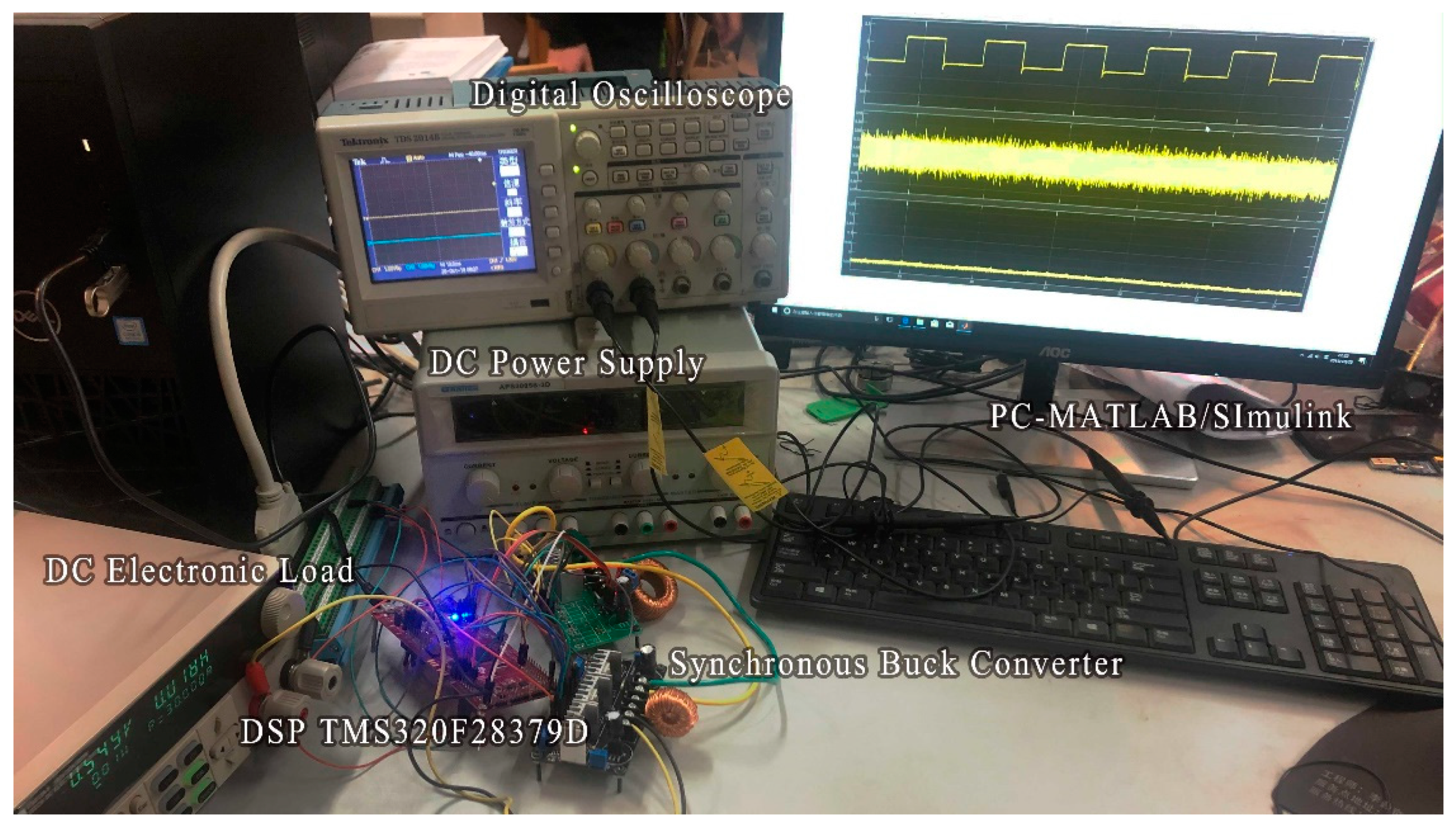
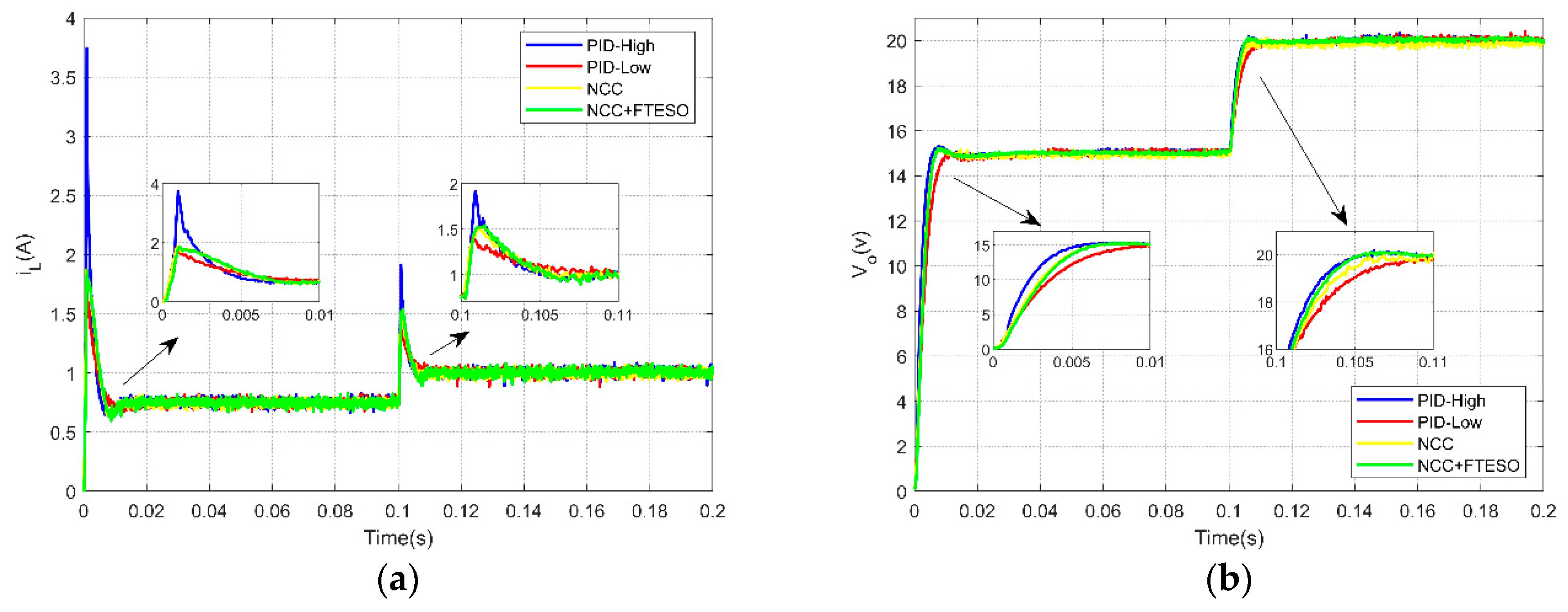
4. Implementation and Validation

In this section, the feasibility and effectiveness of the proposed nonsmooth control algorithm was validated by using a DC–DC synchronous buck converter experimental platform. The experimental platform is shown in Figure 3, including: two DC-DC synchronous buck converters (one is used to realize the sudden change of input voltage), DSP LaunchPad TMS320F28379D (used as a control platform), a DC power supply, digital oscilloscope, DC electronic load, PC-MATLAB/Simulink (used to obtain the data from the sensors for monitoring). The synchronous buck converter in this experiment is controlled by a basic PWM gate drive, and the frequency of PWM drive signals generated by DSP is 20 kHz. Similarly, the sampling frequency of the control system is also 20 kHz. The nominal values of its parameters are listed in

Table 1. Parameters of the DC–DC synchronous buck converter.

Descriptions	Parameters	Nominal Values
Input Voltage	E	30 (V)
Desired Out Voltage	$V_r$	15 (V)
Inductance	L	15 (mH)
Capacitance	C	470 (μF)
Load Resistance	R	20 (Ω)

.

In order to evaluate the advantages of the proposed controller, the widely used PID controller was selected for comparison. At the same time, to verify the disturbance rejection ability of the proposed method, the nonsmooth current-constrained controller was also employed in the experiment. The proper parameters of the selected controllers are listed in

Table 2. Control parameters.

Controllers	Parameters
NCC + FTESO	l = 200, M = 2, $k_1=8\times {10}^5$, $k_2=1.3\times {10}^4$, ${\gamma }_1$ = 1/2, ${\gamma }_2$ = 2/3, ${\gamma }_3$ = 1, ${\beta }_{11}=120$, ${\beta }_{12}=5400$, ${\beta }_{21}=400$, ${\beta }_{22}=8.2\times {10}^4$
NCC	l = 200, M = 2, $k_1=8\times {10}^5$, $k_2=1.3\times {10}^4$, ${\gamma }_1$ = 1/2, ${\gamma }_2$ = 2/3, ${\gamma }_3$ = 1
PID (High gain)	$k_p=8$, $k_i=500$, $k_d=43$
PID (Low gain)	$k_p=3$, $k_i=320$, $k_d=38$

.

As described in Table 2, the PID controller selected a group of high-gain parameters to obtain a faster dynamic response speed, and a group of low-gain parameters to meet the current constraints ($\left|i_L\right|\le 2\mathrm{A}$). At the same time, in order to have a fair comparison, the parameters of the proposed method were selected at the same values as those of nonsmooth current-constrained control (NCC). In this paper, experiments were carried out under three conditions: different reference voltages, a sudden load change and a sudden input voltage change. The latter two can show the improvement of the matched/unmatched disturbances rejection ability of the proposed controller.

Case 1 (Dynamical performance under different reference voltages): In this case, the reference voltage of the synchronous buck converter changed from 15 V to 20 V at 0.1 s, and the other parameters remained the same as the nominal values. It can be seen from the output voltage and inductance current response curves in Figure 4 that the four controllers could stabilize the output voltage to the reference value. Among them, PID (High gain) had a shorter convergence time, but also had a larger transient inductor current, especially in the start-up phase, its value can reach nearly 3.8 A, which would damage the hardware circuit. Although PID (Low gain) could meet the current constraints, the convergence time of output voltage was greatly increased. Compared with PID (High gain), the dynamic performance of output voltage of the proposed control method is sacrificed to some extent to guarantee the current constrain, but it still has a short convergence time.

Case 2 (Robustness against sudden load resistance change): In the same way, the load resistance was reduced from 20 Ω to 10 Ω at 0.1 s by a DC electronic load. The response curves of output voltage and inductance current are shown in Figure 5. The traditional PID controllers still recovered the output voltage to 15 V after the sudden change of load resistance happened while the NCC method does not. By adding FTESOs to estimate and compensate the matched/unmatched disturbances, this problem can be solved, moreover the composite controller achieves a shorter recovery time than the PID method.

Case 3 (Robustness against sudden input voltage change): Similarly, only the parameter of input voltage value was reduced from 30 V to 18 V at 0.1 s here. The corresponding output voltage and inductance current curves are shown in Figure 6. It can be observed that NCC + FTESO had better disturbance rejection ability and robustness compared with the NCC method and had shorter recovery time compared with the PID method.

More details about the convergence time and steady state error in different cases are shown in

Table 3. Convergence time in different cases.

Controllers	Start-Up $({\mathit{V}}_{\mathit{r}}:0 \mathit{V}\to 15 \mathit{V})$	Reference Voltage Change $({\mathit{V}}_{\mathit{r}}:15 \mathit{V}\to 20 \mathit{V})$	Load Resistance Change $(\mathit{R}:20 \mathbf{\Omega }\to 10 \mathbf{\Omega })$	Input Voltage Change $(\mathit{E}:15 \mathit{V}\to 20 \mathit{V})$
PID (High gain)	0.0055 (s)	0.0043 (s)	0.0277 (s)	0.0217 (s)
PID (Low gain)	0.0096 (s)	0.0083 (s)	0.0370 (s)	0.0242 (s)
NCC	0.0063 (s)	0.0055 (s)	/	/
NCC + FTESO	0.0063 (s)	0.0046 (s)	0.0207 (s)	0.0097 (s)

and

Table 4. Steady state error in different cases.

Controllers	Start-Up $({\mathit{V}}_{\mathit{r}}:0 \mathit{V}\to 15 \mathit{V})$	Reference Voltage Change $({\mathit{V}}_{\mathit{r}}:15 \mathit{V}\to 20 \mathit{V})$	Load Resistance Change $(\mathit{R}:20 \mathbf{\Omega }\to 10 \mathbf{\Omega })$	Input Voltage Change $(\mathit{E}:15 \mathit{V}\to 20 \mathit{V})$
PID (High gain)	0.10 (V)	0.11 (V)	0.11 (V)	0.10 (V)
PID (Low gain)	0.10 (V)	0.10 (V)	0.11 (V)	0.09 (V)
NCC	0.07 (V)	0.13 (V)	/	/
NCC + FTESO	0.06 (V)	0.08 (V)	0.09 (V)	0.08 (V)

.

5. Conclusions

In this paper, a nonsmooth current-constrained control method for a DC-DC synchronous buck converter with two finite-time extended state observers is proposed. The proposed control method used the barrier Lyapunov function to satisfy the current constraints. Then the FTESOs were used to estimate the integrated matched/unmatched disturbances and considered in the design process of the controller to achieve the better disturbance rejection ability and robustness. The feasibility of the proposed method has been verified by experimental results. Since it is still a difficult work to define a prior uncertainty bound in the actual converter system, this will be the focus of our future research [39,40,41].

References

1. Erickson, R.W.; Maksimovic, D. Fundamentals of Power Electronics, 2nd ed.; Kluwer Academic: Norwell, MA, USA, 2001; ISBN 9781475705591. [Google Scholar]
2. Wang, J.; Zhang, C.; Li, S.; Yang, J.; Li, Q. Finite-time output feedback control for PWM-based DC–DC buck power converters of current sensorless mode. IEEE Trans. Control Syst. Technol. 2016, 25, 1359–1371. [Google Scholar] [CrossRef]
3. Wang, J.; Li, S.; Yang, J.; Wu, B.; Li, Q. Finite-time disturbance observer based non-singular terminal sliding-mode control for pulse width modulation based DC–DC buck converters with mismatched load disturbances. IET Power Electron. 2016, 9, 1995–2002. [Google Scholar] [CrossRef]
4. Yang, J.; Wu, B.; Li, S.; Yu, X. Design and qualitative robustness analysis of an DOBC approach for DC-DC buck converters with unmatched circuit parameter perturbations. IEEE Trans. Circuits Syst. I Regul. Pap. 2016, 63, 551–560. [Google Scholar] [CrossRef]
5. Wang, Z.; Li, S.; Wang, J.; Li, Q. Robust control for disturbed buck converters based on two GPI observers. Control Eng. Pract. 2017, 66, 13–22. [Google Scholar] [CrossRef]
6. Wei, Y.; Qiu, J.; Karimi, H.R.; Ji, W. A novel memory filtering design for semi-Markovian jump time-delay systems. IEEE Trans. Syst. Man Cybern. Syst. 2017, 48, 2229–2241. [Google Scholar] [CrossRef]
7. Wei, Y.; Qiu, J.; Shi, P.; Wu, L. A piecewise-markovian lyapunov approach to reliable output feedback control for fuzzy-affine systems with time-delays and actuator faults. IEEE Trans. Cybern. 2017, 48, 2723–2735. [Google Scholar] [CrossRef] [PubMed]
8. Yan, Y.; Zhang, C.; Liu, C.; Yang, J.; Li, S. Disturbance rejection for nonlinear uncertain systems with output measurement errors: Application to a helicopter model. IEEE Trans. Ind. Inf. 2019. [Google Scholar] [CrossRef]
9. Roy, S.; Baldi, S. On reduced-complexity robust adaptive control of switched Euler–Lagrange systems. Nonlinear Anal. Hybrid Syst. 2019, 34, 226–237. [Google Scholar] [CrossRef]
10. Wei, Y.; Yu, H.; Karimi, H.R.; Joo, Y.H. New approach to fixed-order output-feedback control for piecewise-affine systems. IEEE Trans. Circuits Syst. I Regul. Pap. 2018, 65, 2961–2969. [Google Scholar] [CrossRef]
11. Kumar, G.; Kumar, A.; Jakka, R. The particle swarm modified quasi bang-bang controller for seismic vibration control. Ocean Eng. 2018, 166, 105–116. [Google Scholar] [CrossRef]
12. Kim, H.; Kim, J.; Shim, M.; Jung, J.; Park, S.; Kim, C. A digitally controlled DC-DC buck converter with bang-bang control. In Proceedings of the 2014 International Conference on Electronics, Information and Communications (ICEIC), Kota Kinabalu, Malaysia, 5–18 January 2014; pp. 1–2. [Google Scholar]
13. Roy, S.; Roy, S.B.; Lee, J.; Baldi, S. Overcoming the underestimation and overestimation problems in adaptive sliding mode control. IEEE/ASME Trans. Mechatron. 2019, 24, 2031–2039. [Google Scholar] [CrossRef] [Green Version]
14. Roy, S.; Baldi, S.; Fridman, L.M. On adaptive sliding mode control without a priori bounded uncertainty. Automatica 2019. [Google Scholar] [CrossRef]
15. Zhou, H.; Chen, R.; Zhou, S.; Liu, Z. Design and Analysis of a Drive System for a Series Manipulator Based on Orthogonal-Fuzzy PID Control. Electronics 2019, 8, 1051. [Google Scholar] [CrossRef] [Green Version]
16. Poyyamani Sunddararaj, S.; Rangarajan, S.S.; Gopalan, S. Neoteric Fuzzy Control Stratagem and Design of Chopper fed Multilevel Inverter for Enhanced Voltage Output Involving Plug-In Electric Vehicle (PEV) Applications. Electronics 2019, 8, 1092. [Google Scholar] [CrossRef] [Green Version]
17. Liu, X.; Cao, J.; Xie, C. Finite-time and fixed-time bipartite consensus of multi-agent systems under a unified discontinuous control protocol. J. Franklin Inst. 2017, 356, 734–751. [Google Scholar] [CrossRef]
18. Li, D.; Cao, J. Fuzzy finite-time stability of chaotic systems with time-varying delay and parameter uncertainties. Math. Prob. Eng. 2015, 2015. [Google Scholar] [CrossRef] [Green Version]
19. Bhat, S.P.; Bernstein, D.S. Continuous finite-time stabilization of the translational and rotational double integrators. IEEE Trans. Autom. Control 1998, 43, 678–682. [Google Scholar] [CrossRef] [Green Version]
20. Hong, Y.; Huang, J.; Xu, Y. On an output feedback finite-time stabilization problem. IEEE Trans. Autom. Control 2001, 46, 305–309. [Google Scholar] [CrossRef] [Green Version]
21. Guo, T.; Wang, Z.; Wang, X.; Li, S.; Li, Q. A simple control approach for buck converters with current-constrained technique. IEEE Trans. Control Syst. Technol. 2017, 27, 418–425. [Google Scholar] [CrossRef]
22. Ma, F.-F.; Chen, W.-Z.; Wu, J.-C. A monolithic current-mode buck converter with advanced control and protection circuits. IEEE Trans. Power Electron. 2007, 22, 1836–1846. [Google Scholar] [CrossRef]
23. Sun, Z.; Guo, T.; Yan, Y.; Wang, X.; Li, S. A composite current-constrained control for permanent magnet synchronous motor with time-varying disturbance. Adv. Mech. Eng. 2017, 9. [Google Scholar] [CrossRef] [Green Version]
24. Gilbert, E.G.; Tan, K.T. Linear systems with state and control constraints: The theory and application of maximal output admissible sets. IEEE Trans. Autom. Control 1991, 36, 1008–1020. [Google Scholar] [CrossRef] [Green Version]
25. Mayne, D.; Schroeder, W. Nonlinear control of constrained linear systems: Regulation and tracking. In Proceedings of the 1994 33rd IEEE Conference on Decision and Control, Lake Buena Vista, FL, USA, 14–16 December 1994; pp. 2370–2375. [Google Scholar]
26. Eaton, J.W.; Rawlings, J.B. Model-predictive control of chemical processes. Chem. Eng. Sci. 1992, 47, 705–720. [Google Scholar] [CrossRef]
27. Lazar, M.; Heemels, W.; Roset, B.; Nijmeijer, H.; Van Den Bosch, P. Input-to-state stabilizing sub-optimal NMPC with an application to DC–DC converters. Int. J. Robust Nonlin. Control 2008, 18, 890–904. [Google Scholar] [CrossRef]
28. Yang, J.; Zheng, W.X.; Li, S.; Wu, B.; Cheng, M. Design of a prediction-accuracy-enhanced continuous-time MPC for disturbed systems via a disturbance observer. IEEE Trans. Ind. Electron. 2015, 62, 5807–5816. [Google Scholar] [CrossRef]
29. Tee, K.P.; Ge, S.S.; Tay, F.E.H. Adaptive control of electrostatic microactuators with bidirectional drive. IEEE Trans. Control Syst. Technol. 2008, 17, 340–352. [Google Scholar]
30. Won, D.; Kim, W.; Shin, D.; Chung, C.C. High-gain disturbance observer-based backstepping control with output tracking error constraint for electro-hydraulic systems. IEEE Trans. Control Syst. Technol. 2014, 23, 787–795. [Google Scholar] [CrossRef]
31. Chen, W.-H.; Yang, J.; Guo, L.; Li, S. Disturbance-observer-based control and related methods—An overview. IEEE Trans. Ind. Electron. 2015, 63, 1083–1095. [Google Scholar] [CrossRef] [Green Version]
32. Zhao, L.; Li, Q.; Liu, B.; Cheng, H. Trajectory tracking control of a one degree of freedom manipulator based on a switched sliding mode controller with a novel extended state observer framework. IEEE Trans. Syst. Man Cybern. Syst. 2017, 49, 1110–1118. [Google Scholar] [CrossRef]
33. Li, B.; Hu, Q.; Yang, Y. Continuous finite-time extended state observer based fault tolerant control for attitude stabilization. Aerosp. Sci. Technol. 2019, 84, 204–213. [Google Scholar] [CrossRef]
34. Rosier, L. Homogeneous Lyapunov function for homogeneous continuous vector field. Syst. Contr. Lett. 1992, 19, 467–473. [Google Scholar] [CrossRef]
35. Du, H.; He, Y.; Cheng, Y. Finite-time synchronization of a class of second-order nonlinear multi-agent systems using output feedback control. IEEE Trans. Circuits Syst. I Regul. Pap. 2014, 61, 1778–1788. [Google Scholar] [CrossRef]
36. Xu, B.; Shi, Z.; Sun, F.; He, W. Barrier Lyapunov function based learning control of hypersonic flight vehicle with AOA constraint and actuator faults. IEEE Trans. Cybern. 2018, 49, 1047–1057. [Google Scholar] [CrossRef] [PubMed]
37. Yu, J.; Zhao, L.; Yu, H.; Lin, C. Barrier Lyapunov functions-based command filtered output feedback control for full-state constrained nonlinear systems. Automatica 2019, 105, 71–79. [Google Scholar] [CrossRef]
38. Khalil, H.K. Nonlinear Systems, 3rd ed.; Prentice-Hall: Upper Saddle River, NJ, USA, 2002; ISBN 0130673897. [Google Scholar]
39. Roy, S.; Baldi, S. A Simultaneous Adaptation Law for a Class of Nonlinearly Parametrized Switched Systems. IEEE Control Syst. Lett. 2019, 3, 487–492. [Google Scholar] [CrossRef] [Green Version]
40. Roy, S.; Kar, I.N.; Lee, J.; Tsagarakis, N.G.; Caldwell, D.G. Adaptive-robust control of a class of EL systems with parametric variations using artificially delayed input and position feedback. IEEE Trans. Control Syst. Technol. 2017, 27, 603–615. [Google Scholar] [CrossRef] [Green Version]
41. Roy, S.; Kar, I.N. Adaptive-Robust Control with Limited Knowledge on Systems Dynamics: An Artificial Input Delay Approach and Beyond; Springer Nature: Singapore, 2019; ISBN 9789811506390. [Google Scholar]
Figure 1. Average model circuit of synchronous buck converter: (a) Circuit topology of synchronous buck converter; (b) u = 1 ; (c) u = 0 .
Electronics 09 00016 g001
Figure 2. The controller design of the synchronous buck converter.
Electronics 09 00016 g002
Figure 3. The experimental platform of the DC–DC synchronous buck converter.
Electronics 09 00016 g003
Figure 4. Inductance current and output voltage response curves of PID, NCC, and NCC + FTESO under different reference voltages. (a) Inductance current; (b) output voltage.
Electronics 09 00016 g004
Figure 5. Inductance current and output voltage response curves of PID, NCC, and NCC +FTESO under a sudden load resistance change. (a) Inductance current; (b) output voltage.
Electronics 09 00016 g005
Figure 6. Inductance current and output voltage response curves of PID, NCC, and NCC + FTESO under a sudden input voltage change. (a) Inductance current; (b) output voltage.
Electronics 09 00016 g006