Article

Mobilities in Network Topology and Simulation Reproducibility of Sightseeing Vehicle Detected by Low-Power Wide-Area Positioning System

1
Department of Electronic Systems Engineering, The University of Shiga Prefecture, 2500 Hassakacho, Hikone, Shiga 522-8533, Japan
2
Regional ICT Research Center for Human, Industry and Future, The University of Shiga Prefecture, 2500 Hassakacho, Hikone, Shiga 522-8533, Japan
3
Eagle Electronics Corp, 1555-1 Minamikawasecho, Hikone, Shiga 522-0222, Japan
*
Author to whom correspondence should be addressed.
Electronics 2020, 9(1), 116; https://doi.org/10.3390/electronics9010116
Submission received: 30 October 2019 / Revised: 6 December 2019 / Accepted: 31 December 2019 / Published: 7 January 2020
(This article belongs to the Section Networks)

Abstract

:
Vehicle mobilities for passengers in a city’s downtown area or in the countryside are significant points to characterize their functions and outputs. We focus on commercial sightseeing vehicles in a Japanese city where many tourists enjoy sightseeing. Such mobilities and their visualizations make tourist activities smoother and richer. We design and install a low-power, wide-area positioning system on a rickshaw, which is a human-pulled, two- or three-wheeled cart, and monitor its mobility in Hikone City. All the spatial locations, which are recorded in a time sequence on a cloud server, are currently available as open data on the internet. We analyze such sequential data using graph topology, which reflects the information of corresponding geographical maps, and reproduce it in cyberspace using an agent-based model with similar probabilities to the accumulated rickshaw records from one spatial node to another. Although the numerical results of the agent traced in a simulated city are partially consistent with the rickshaw’s record, we identify some significant differences. We conclude that the rickshaw’s mobility observed at the actual sightseeing sites is partially in the random motion; some cases are strongly biased by memory routes. Such non-randomness in the rickshaw’s mobility indicates the existence of specific features in tourism sources that are identified for each sightseeing activity and affected by local sightseeing resources.

Graphical Abstract

1. Introduction

Although the mobilities of vehicles are somewhat limited by their hardware, their drivers and passengers generally determine their mobility and where to go. Under the control of local traffic rules, their mobilities indicate a vehicle’s social functions and uses. As well as human geographical motions [1,2,3,4,5], vehicle mobilities have been scrutinized to understand their outputs in traffic transportations [6,7].
To detect and visualize such mobilities, many electronic tools have been designed and installed on vehicles and other movable equipment [8,9,10,11,12,13,14]. For instance, many kinds of mobile phones include an antenna and a device for global navigation satellite systems (GNSSs) [15,16,17]. Our daily activities can be recorded when such components are operational. In our study on the detection of vehicle functions in tourism, the temporal sequential data of spatial locations every several minutes are suitable for recording the traces of vehicle mobilities, because the typical characteristic times of the behaviors are several tens of minutes. GNSS or global positioning systems (GPSs) provide the antenna (and device) locations as longitude and latitude values, whose bit information is not so large even if 10 m spatial resolution is required [5,12,15,16,17,18]. Therefore, the capacity of high-speed wireless telecommunications such as Wi-Fi (IEEE 802.11 protocol standards) is too large in the category of wireless local area networking. Since a data rate with very small capacity is adequate and reasonable, we selected a low-power, wide-area (LPWA) network [18,19,20] that allows long-range wireless telecommunication at a low bit rate with low-power consumption, which is suitable for the Internet-of-Things (IoT) [21,22,23,24], i.e., objects that are connected to the internet. Then, the positioning system data are transferred by LPWA to a cloud data server every several minutes, where the dataset is accumulated; its unit data are composed of digit numbers for time, longitude, and latitude. Due to recent progress in IoT technology, large amounts of data are accumulated and available in healthcare systems, environmental monitoring systems, and structural health monitoring systems (SHMs) [24], etc. For instance, SHMs automatically detect in time the temporal conditions of such urban and rural infrastructures as buildings, bridges, and railway tracks. Although our purpose in this research is different from that of SHM, SHM and other IoT systems share hardware and software elements, like sensors and LPWA networks, inviting possible collaboration.
After storing the accumulated data of the vehicles in the cloud data server, we can analyze the functions and the outputs from their spatiotemporal traces. Our study shown here is not only for the electronic design of the hardware but also for a total system to analyze vehicle mobilities that enables us to obtain knowledge on the social roles of given vehicles. In this study, we focus on data from commercial sightseeing vehicles. In Japan, the amount of overseas tourists has been rapidly increasing, and many traffic vehicles support such sightseeing activities in cities with touristic resources. For instance, 90% of the tourists in the Shiga prefecture are on day trips from Kyoto or Osaka [25], and the local economic benefits are limited compared to other cases that include hotels and overnight stays. With limited time for one visit, smooth and convenient traffic conditions might increase the motivation of tourists, increasing their financial outlays and the amount of time they spend in the city.
In the Shiga prefecture, in Japan’s Kansai area, five railway companies operate trains and several bus companies have local routes. Taxis comprise another important vehicle system that obviously operates without fixed routes. In comparison with such modern vehicles, the transportation properties of rickshaws [26,27] provide significant advantages. Operated by humans, although the speed of rickshaws resembles human walking or jogging, their small size makes them more flexible in crowded places and allows them to get closer to tourist targets. Another important feature which we are now focusing on is that riding in rickshaws in modern Japan is limited to tourism instead of business or daily commuting; rather, railways, buses, and taxies are used for business and daily commuting.
Due to their unique features and functions for making tourists more comfortable, a commercial vehicle’s mobility for sightseeing uses, a rickshaw, is worth analyzing to clarify its features. We analyze the data of their traces on a cloud server with the graphical approximation of rickshaw routes using networking or graph representation and simulate rickshaw motions in cyberspace with similar conditions to a given area using an agent-based model. Agent-based models are widely used to simulate movable objects in hypothetical situations [28,29,30,31,32]. For instance, multi-agent simulations can predict epidemic dissemination in a given social space from a local area to an international region, where an agent corresponds to one person [28]. An agent who imitates a movable item is in a probabilistic or stochastic process and moves randomly without specific restrictions in hypothetical space. In our study, this hypothetical space is set similarly to the graph topology created from geographical data, and we compare the numerical results calculated in agent-based simulations with actual records of rickshaws on the server to validate the assumption in the model calculation and extract specific features unique to a given sightseeing area. That is, agent-based simulations are likely to show random motions occurring in a stochastic process, but in the rickshaw’s real motions, some fractions of motions are probably outside of such random motions. This difference between agent-based simulations and actual monitoring will reveal this fraction in rickshaw mobility: non-random scheduled motions affected by external biases.
In this study, we design and create, for analyzing vehicle mobilities in a sightseeing area, a total system which includes an electronic device for the positioning system, graph representation of geographical information, and agent-based simulations for the vehicles. We focus on rickshaws in the Hikone area [33,34] since we can capture good estimates of their capabilities and functions to simulate local sightseeing. Hikone has such historical treasures as a castle, temples, gardens, and other touristic monuments. Around such sightseeing spots, tourists can experience rich traditional Japanese streets, restaurants, souvenir shops, and hotels. The results of our analysis on rickshaw data in Hikone show that rickshaw mobilities include both random and biased elements, which can be distinguished to characterize the features of corresponding sightseeing areas. Our study clarifies the rickshaw mobilities in a network of sightseeing spots and their reproducibility in a simulation model, and we detect both random and biased (scheduled) motions. This fact suggests that rickshaw passengers enjoy arbitrary sightseeing spots that reflect their own tastes in some cases; in other cases, they prefer biased chain-like visits based on recommendations in advance. In Section 2, we introduce our methods for electronic device design, the processes for graph representations, and an algorithm of the agent-based model. In Section 3, we show the spatiotemporal data of rickshaws recorded on a cloud server, and analyze them using an agent-based model. We summarize our study in Section 4.

2. Methods

2.1. LPWA Positioning System with Cloud Data Storage

We designed a LPWA positioning system (EUOX18X31-01, Eagle Electronics Corp., Shiga, Japan) shown in Figure 1 and described below. Figure 1a displays the complete system of our device, the telecommunication path, storage on the cloud server, and open-data visualization on the internet, and Figure 1b shows our device’s module design installed on a rickshaw. A GPS module communicates to GPS satellites by a patch antenna and detects the longitude and latitude values of the system’s current position. For stable communication, outdoor uses are preferred, which is enabled by sealing the entire system in a box. In addition to the acquisition of GPS data, we collected the following two occupation states of passengers: the operation state with passengers (boarding) and the vacancy state (free), in which the rickshaw is usually stopped and waiting for new passengers.
LPWA is a long-distance, low-rate, low-power telecommunication scheme. In our system, we installed a Sigfox module for data transfer to the Sigfox data server [35]. The Sigfox system uses an ultra-narrow-band scheme at 920 MHz, which allows low-consumption electric power and long-distance telecommunication with high receiver sensitivity. Although the data rate is not very high (up to 100 bps), data transfer from a module to a base station is feasible up to 50 km.
In our designed device, one data packet sent to the Sigfox data server consists of 12 hexadecimal digits: 4 for longitude, 4 for latitude, 1 for occupation states, 1 for the operational voltage in the device, and 2 preliminary digits for an additional use. This LPWA module sends one data packet every five minutes within several seconds for data transfer. After the transfer to the Sigfox server, the data are retransferred to a commercial cloud server, which stores all the datasets in time sequences. This second data transfer takes place every five minutes, and the time information is added to the longitude and latitude data, which comprise a complete dataset for one timing point.
To operate the above processes in the module, an Arduino microprocessor links to the GPS module, the occupation signal connector, and the LPWA module. The microprocessor controls the repetitive sequence for one series of data acquisition and transfer, i.e., positioning by the GPS module, detection of the occupation states, and the LPWA transfer, including its repetition time that was set to five minutes. The total time required for one sequential procedure for positioning and recording is less than 15 s, which is sufficiently short in comparison to the refreshment intervals (five minutes). As we will show data on rickshaw velocities below, its motion is slow and these time spans (15 s for positioning responding time and five minutes for repetition intervals) are appropriate to trace it with specific mobilities. For each positioning sensor, one mobile battery (PB-N51, AUKEY) is attached to the sealed box. Operation for a few days is possible on one battery charge. A sealed box with a mobile battery was installed on a rickshaw.

2.2. Graph Display Based on Geographic Map

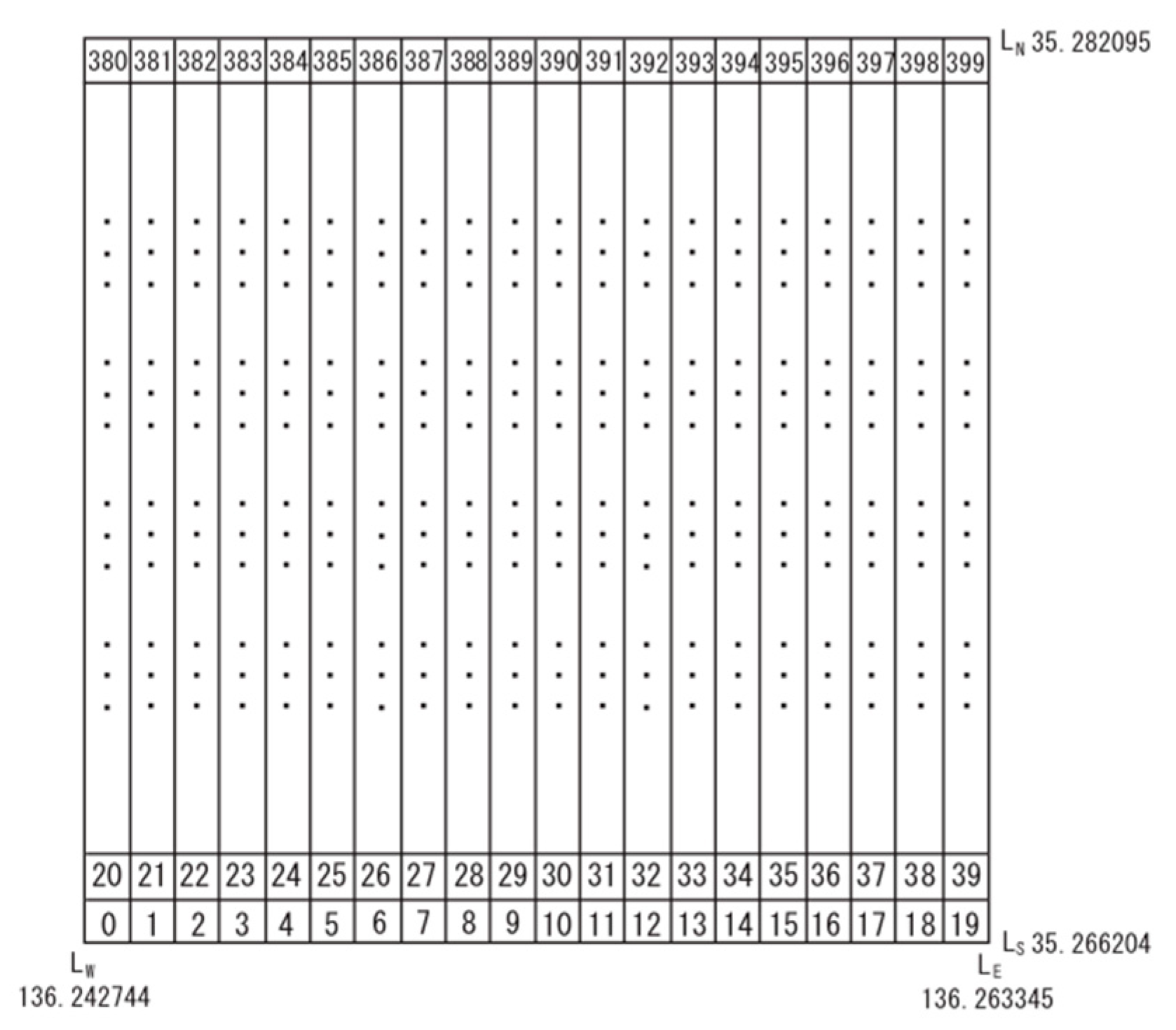
To visualize a rickshaw’s mobility, we made the following graph representation for its routes. First, we converted the two-dimensional geographic information composed of the latitude for y axis and the longitude for x axis into digitized rectangular meshes (see Appendix A and Figure A1). Our target area is Hikone [33,34] in the Shiga prefecture. The following are the recorded values: longitude ranges from 136.242744 to 136.263345 degrees and latitude ranges from 35.266204 to 35.282095 degrees. The digitized rectangular mesh is 0.00079455 by 0.00103005 degrees or 88.4 by 93.6 m, and each mesh is named sequentially (Figure A1), whose numbers represent the node number in a graph described below. Second, we set the linkages between these meshes and real locations in Hikone. Rickshaws [36] are operated mainly along the streets that are displayed in a local geographical map. We converted such map information for automobiles onto a graph composed of nodes and directed edges. Note that these nodes match the previously defined meshes. The directed edges, which are between the nodes, are usually dual-directional unless they are along one-way streets.
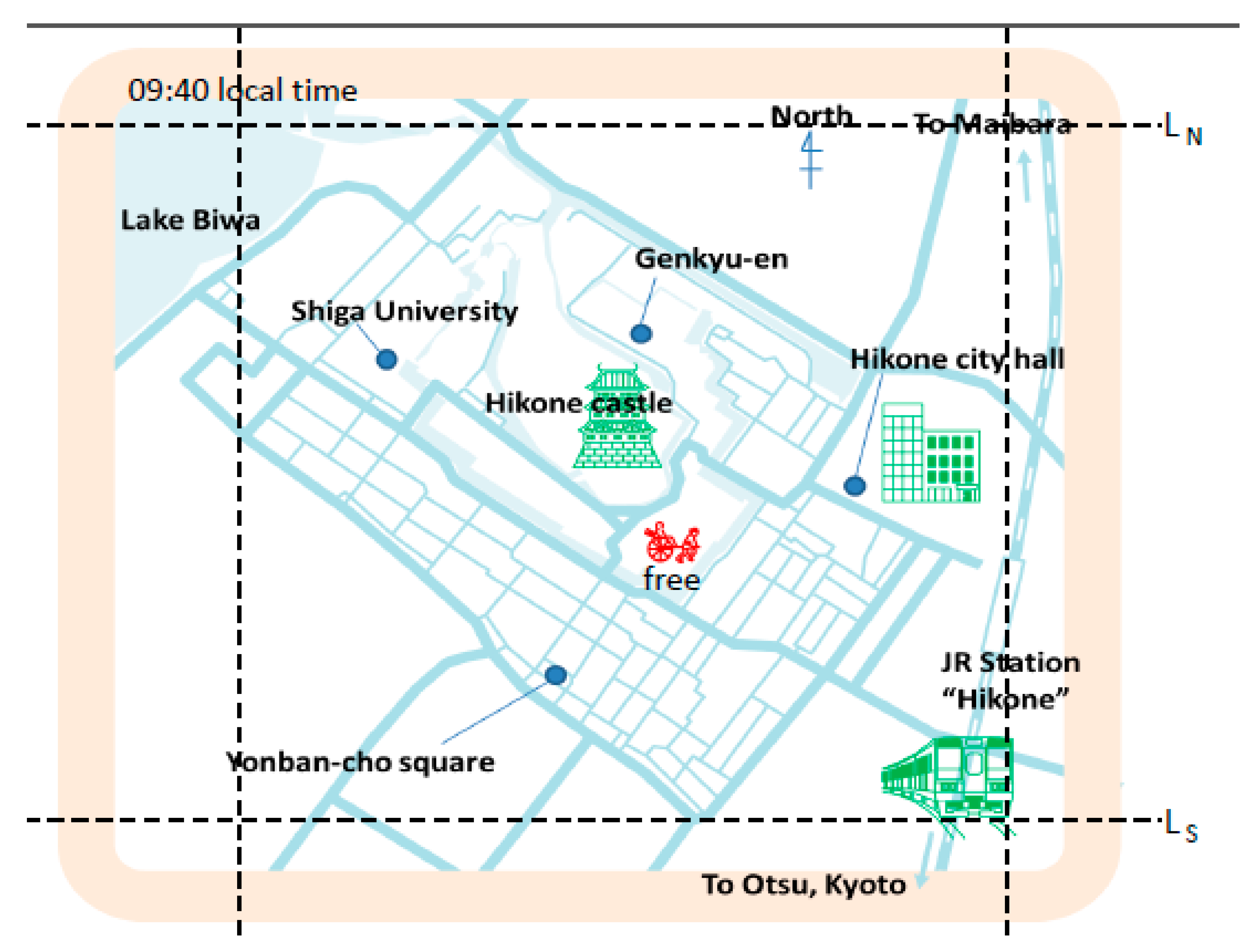
Figure 2 shows a current rickshaw route as open data on the internet with a simplified geographical map [37], which is available to tourists through mobile terminals. When a node is located next to a sightseeing spot like a castle, a temple/shrine, an archaeological site, a souvenir shop, a restaurant, or a good view for such sightseeing spots (Figure 2), a rickshaw’s traces in the cloud-server record frequently overlap these spots. If a node is along a shortcut between nearby sightseeing-spot-nodes, the rickshaw’s traces also frequently overlap it.

2.3. Numerical Simulation in Agent-Based Model

Based on the graph topology configured by the method shown in Section 2.2, we configured a numerical simulation code in an agent-based model, which is a widely-used approach for epidemic spreading [28], market actions [29], and vehicle sharing [30]. We assume an agent can move in the graph described in Section 2.2; the agent stays at a node and moves to another node along a directed edge every time step. The selection of the next node for a temporal destination at each step depends on the corresponding probability from the current node to the next. The numbers of visits to a given node depends on the probabilities to which the given node is subject and the graph topology that determines the routes along the directed edges. Our model did not address any memory effects for the selection of the next node. Agents move in a Markov process.

3. Results and Discussion

3.1. Vehicle Traces Derived from Data Stored in the Cloud Server

We recorded the spatiotemporal locations of rickshaws operated in Hikone City [33,34], which includes the famous Hikone Castle. In the Edo Era from the 17th to the 19th century, Hikone’s rulers were allies of the central Japanese governors, and sufficient budgets were continuously consumed around the Hikone Castle. This fact indicates that the tourists visiting Hikone will find many pieces of traditional Japanese heritage as sightseeing areas. Sightseeing spots are scattered over a several kilometers long diameter area, which complicates planning by tourists who might want to cover all of them on foot only in one day. Although local bus routes and taxi services are available, rickshaws [26,27,36] are very attractive since they can enter small places that are inaccessible to buses and taxis. Rickshaw passengers can access interesting sites more conveniently at a speed slightly faster than walkers, as described below. Furthermore, compared with buses and taxies, rickshaw rides are only available for sightseeing uses and directly represent such options.
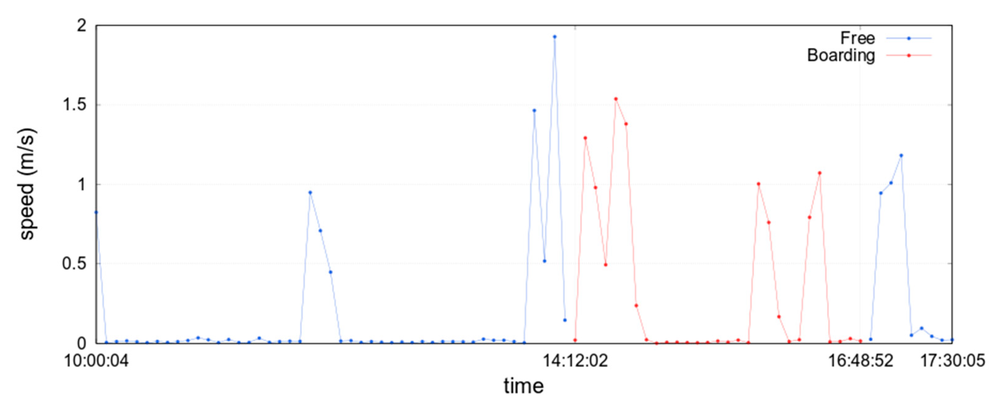
Table 1 shows examples of the accumulated data on the cloud server. Since the data are quite small, they are suitable for LPWA telecommunication. From them, we can derive two elements: operation speed and temporal locations that lead to corresponding nodes. Based on the differences in the locations between two elapsed times, we can easily obtain straight line distances. Since a rickshaw is operated by a human driver at his/her own driving force, its speed is rather low and greatly fluctuates even within the five minute time intervals in the datasets. The time evolution of the calculated speed from the integrated distances for five minutes in Table 1 is shown in Figure 3. The averaged operation velocity was 2.95 km per hour, which resembles a typical walking speed, although slower than jogging. Although passengers in rickshaws cannot quickly reach their final destinations, they will overlook fewer sightseeing opportunities compared to riding in other vehicles; without tiring, they can enjoy the atmosphere around the tourist spots. The data in Table 1 also specify temporal locations that provide corresponding spatial meshes or nodes for all the elapsed times, which is our main interest in this study. For instance, for Table 1, this rickshaw moves from node 149 to node 11 by nodes 231, 149, and 68.
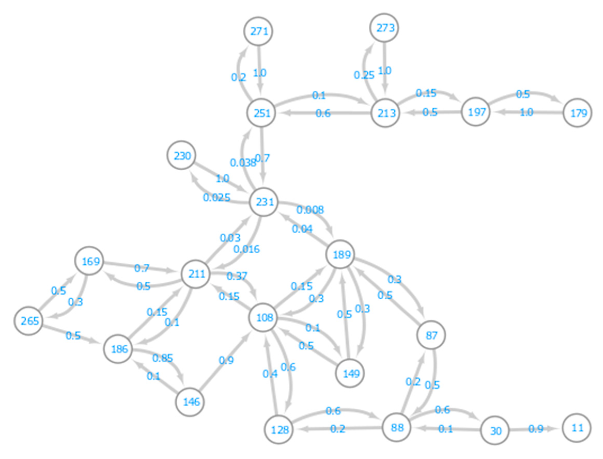
The cloud-sever datasets analyzed here were recorded from one rickshaw that was operated in Hikone for 163 days from 28 November 2018 to 9 May 2019, which is an open dataset available on the internet [37]. After investigating the cloud datasets over a sufficient volume (in our case, for 163 days, which is the maximum for our current analysis), we derived active nodes for rickshaws among all the spatial meshes, and obtained edge information for each node, which includes inward and outward edges from a given node. Figure 4 shows a simple version of a resultant graph or network for rickshaw operations in the Hikone area. Although further details might exist in the individual traces of a daily rickshaw, we configured a graph with 21 nodes to prioritize intuitive understanding. We selected nodes with sequences from the most visited spatial spots, and their classification partially arises from the spatial resolution of the geographical meshes we applied. If the frequently visited spots are adjacent with a distance of less than 100 m, we combined them into one node. Even though the graph is not very complicated, many routes are possible for each tourist in a one-day sightseeing tour with varying interests and concerns, which is now visible in this graph topology. The weight on each edge in Figure 4 represents the tentative probability of the edge selection of the next destination, which is used in Section 3.2. The summation of the weights of the outward edges at one node is 1, except nodes 189 and 231, which have a self-return loop from and to themselves. These self-return edges not shown here possess the rest of the summed probabilities. These two nodes correspond to the waiting and/or stopping spatial spots of the rickshaws.
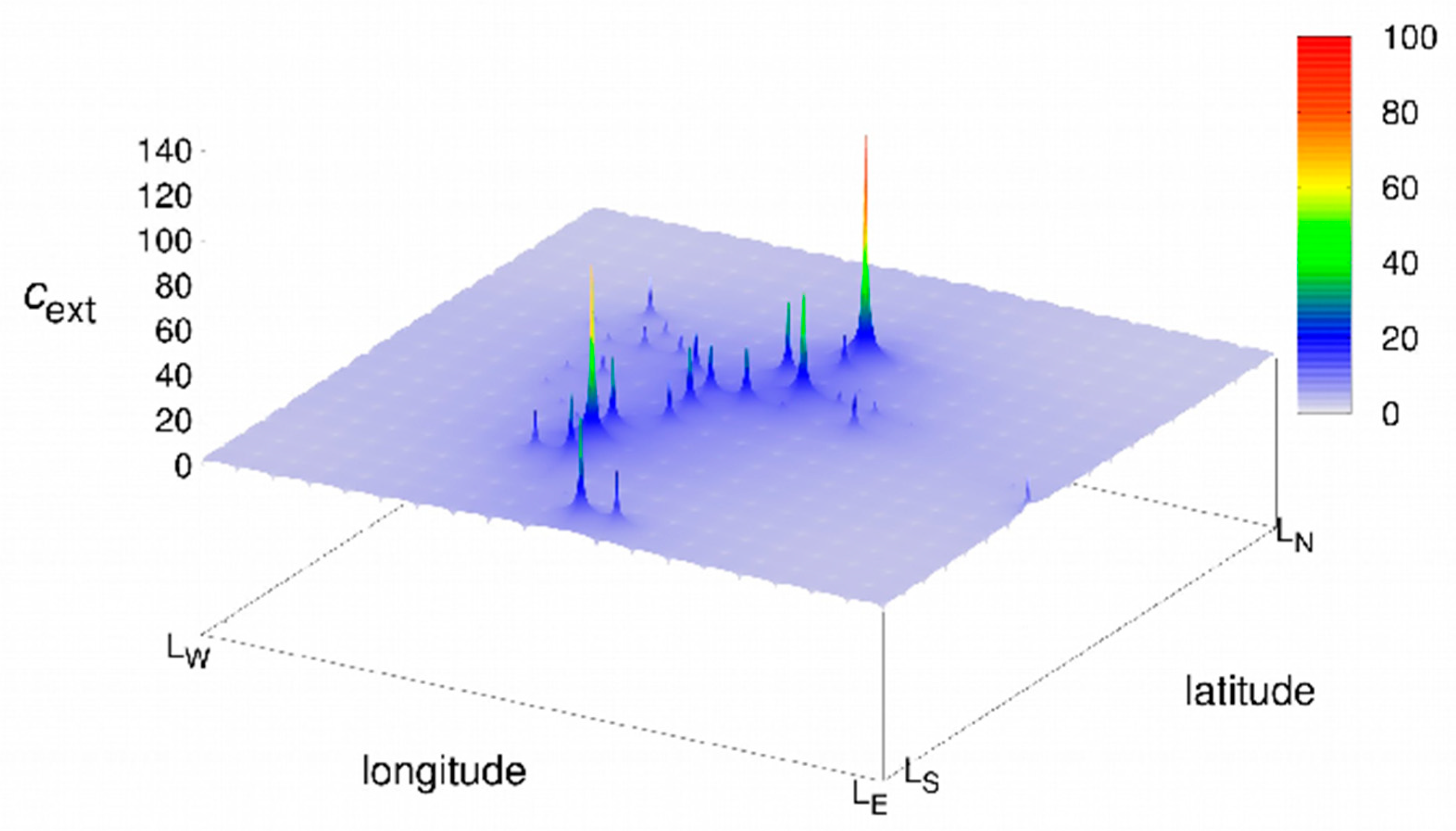
We summed the counts at each spatial mesh unit throughout all the datasets of the 163 operation days and obtained the total number of visits at all the mesh units (Figure 5). Two nodes are not shown here since the counts at these two points have more values than the others: node 11, rickshaw terminal (counts = 693), and node 231, rickshaw stopping primarily to give rides (counts = 3293). That is, except these two points, the total number of visits in Figure 5 reflects the probabilities that the rickshaw is in a mobile state at the corresponding nodes for sightseeing. These values are very informative regarding tourist interests. If the count is high, many tourists are interested in (or receive recommendations from drivers or guidebooks) the corresponding location that probably has famous sightseeing spot(s). For instance, node 271 is one main sightseeing spot near the gate of the Hikone Castle and Genkyu-en (a Japanese garden), and node 108 corresponds to a shopping area called Yonban-cho Square with many souvenir shops and restaurants. However, such information of the counts does not elucidate the popular rickshaw sightseeing routes since we obtain no information about a typical route from the beginning to the end from one ride. Note also that even if the corresponding count is high, such a node might not be associated with sightseeing spots because it might just be a transit area between frequently visited sightseeing spots.

3.2. Predictions by Agent-Based Model and Discussion

In Section 3.1, we investigated the datasets stored on the cloud server and the statistical data with geographical information. To analyze the behaviors of rickshaws that suggest tourist behaviors, we performed agent-based simulations. Agent-based models fundamentally predict probabilistic processes with no memory effects [28,29,30,31,32]; random selections with specific probabilities determine the agent’s next destination. This indicates that numerical results derived by agent-based simulations provide random motions without any biases that might arise from such preset knowledge as recommendations by external information. If the probability set for the selection of the next node is sufficiently accurate, we extract the fraction of randomness from that of the biased or pre-scheduled motions in the rickshaw mobilities.
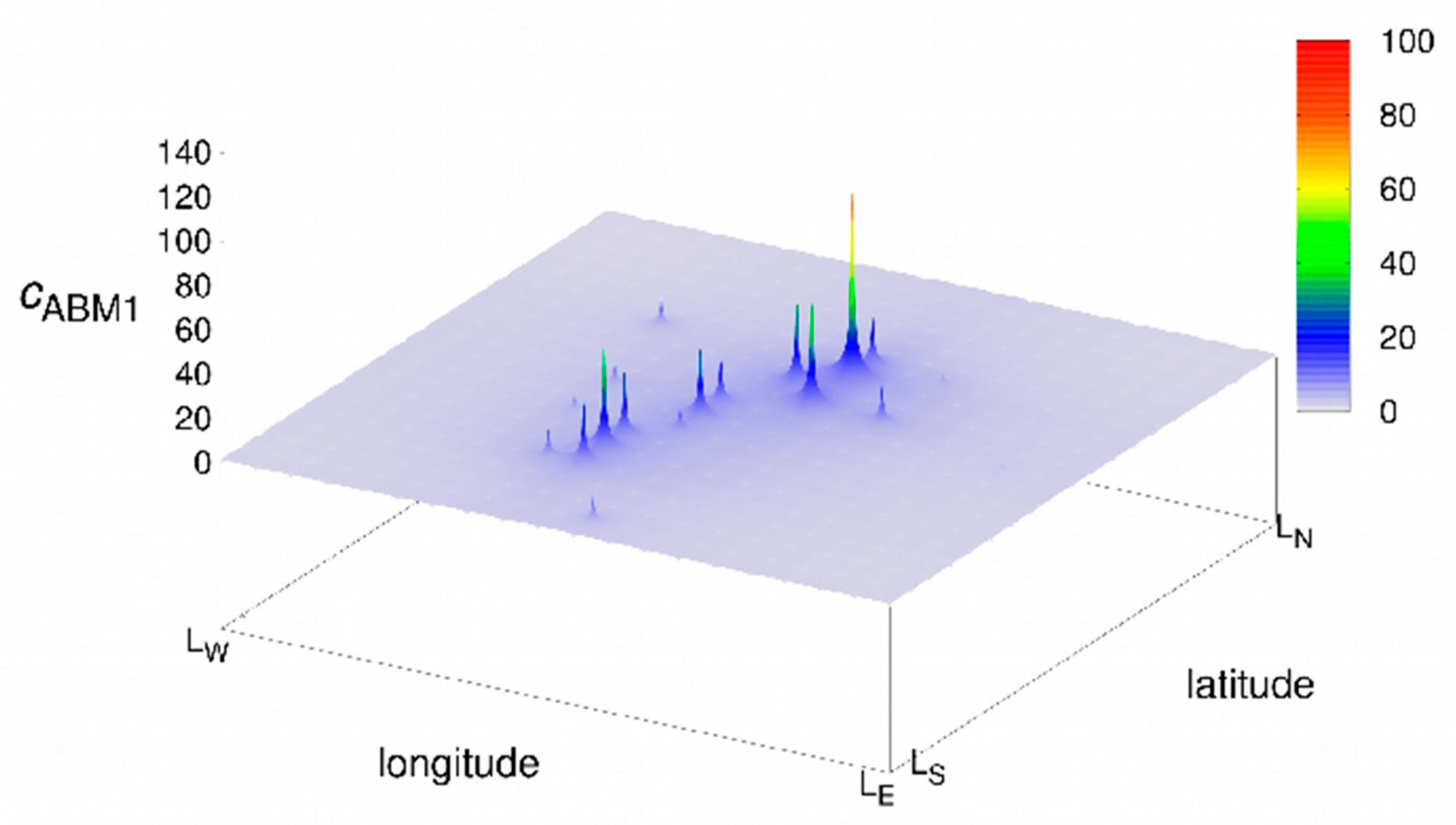
First, a simpler calculation based on the graph in Figure 4 provides a rough insight of the rickshaw’s behaviors, in which two nodes are not shown here: node 11, rickshaw terminal (counts = 50), and node 231, rickshaw stopping primarily for passenger rides (counts = 3554). Here, starting from node 231, 300 agents individually move to the next nodes, and we added the number of visits at each node and compared the numerical result with the monitored one in Figure 5. Note that the moves of one agent are limited up to 15, and an agent stops immediately when it arrives at node 11 (rickshaw terminal). After this procedure, we obtained one of the optimized sets of the mobile probabilities of an agent to the next destination to the first decimal place (Figure 4). Then we performed 4500 simulations using this set of probabilities, where the maximum number of moves is 15, node 11 is the terminal, and the data point at node 231 is removed, which is the rickshaw station where it waits for passengers (the total value of visits: 3239). The spatial patterns of the data distributions in Figure 6 resemble those in Figure 5, indicating that the mobile probabilities set in Figure 4 roughly reproduce those in the actual rickshaw mobilities. However, we found the following significant differences between the experimental result and the model. For instance, node 271 (with the largest value in Figure 5) seems to be a dead end on the geographical map, as in Figure 4, and the counts of the agents in Figure 6 became small. However, in the actual rickshaw count, node 271 had a fairly large value of visits in Figure 5 in comparison with node 251, which is a nearby crossing. Perhaps a shortcut has been overlooked from node 271 to other nodes, or it might have a self-loop edge.
To obtain more accurate reproducibility with a more detailed probabilistic likelihood, we performed another simulation. The graph in Figure 4 is so simple that possible rickshaw routes can be visible and intuitively understood. However, it might be too simple to analyze the details. To investigate further with rigorous examinations using the details of the datasets on the cloud server, we configured the following complicated graph. As shown in Figure 2, we set geometrical meshes in the rickshaw area in Hikone, whose size is 20 by 20 with a unit size in 88.4 × 93.6 m2. Among 400 mesh units, 86 were detected as visiting points in all the datasets and became new nodes, and we counted 594 different patterns of moves between these units, which became new directed edges. We defined the weight of each directed edge that represents the probability to the next destination along such an edge as,
p ( n i + 1 | n i ) = C ( n i + 1 | n i ) C ( n i ) ,
where p(ni+1|ni) is the conditional probability of visits to node ni+1 after node ni, C(ni) is the total count of visits to node ni, and C(ni+1|ni) is the count of visits to node ni+1 just after node ni. We tentatively assume that the stochastic process in this agent model is in a simple Markov chain with a memoryless information source [38].
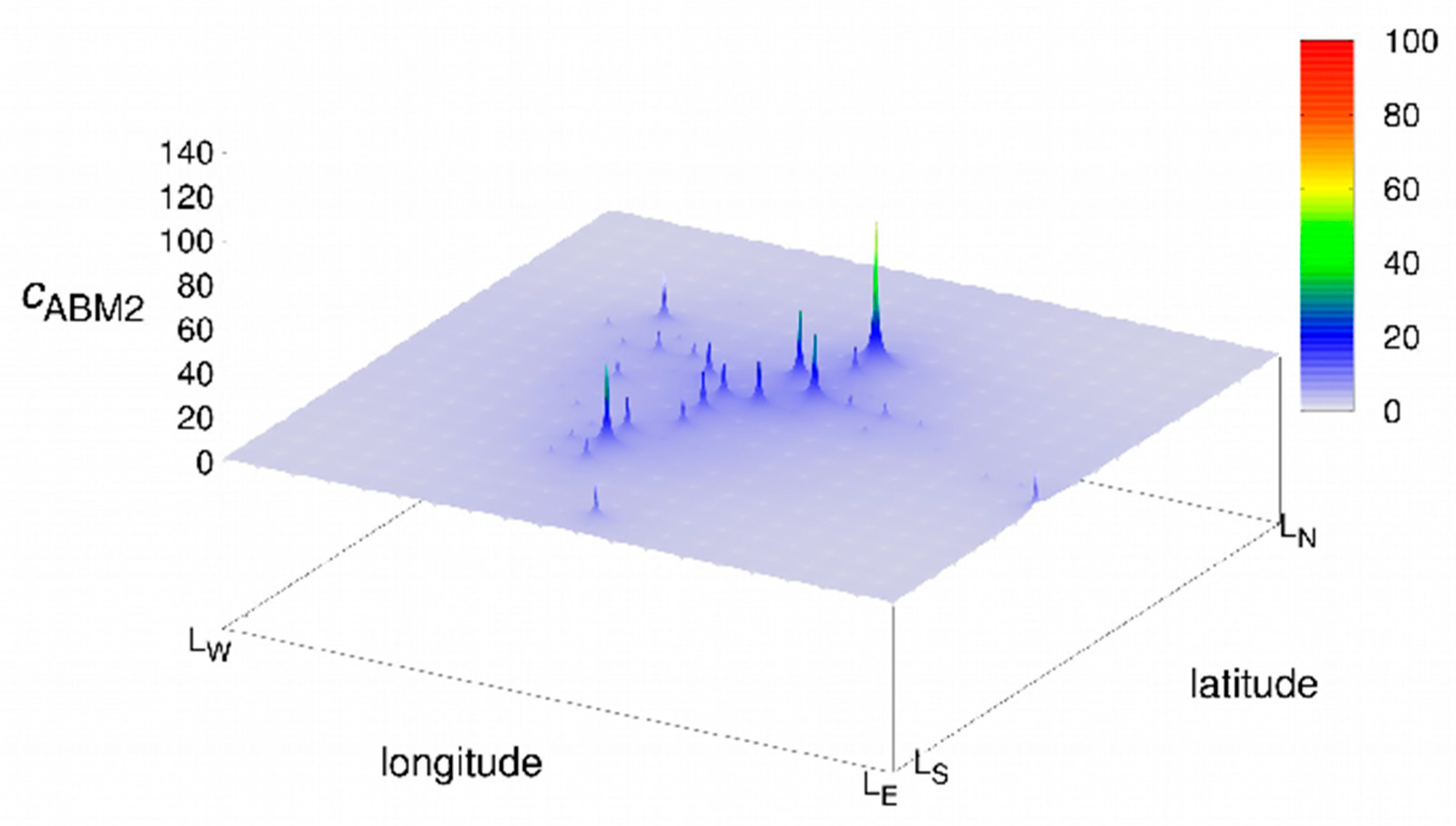
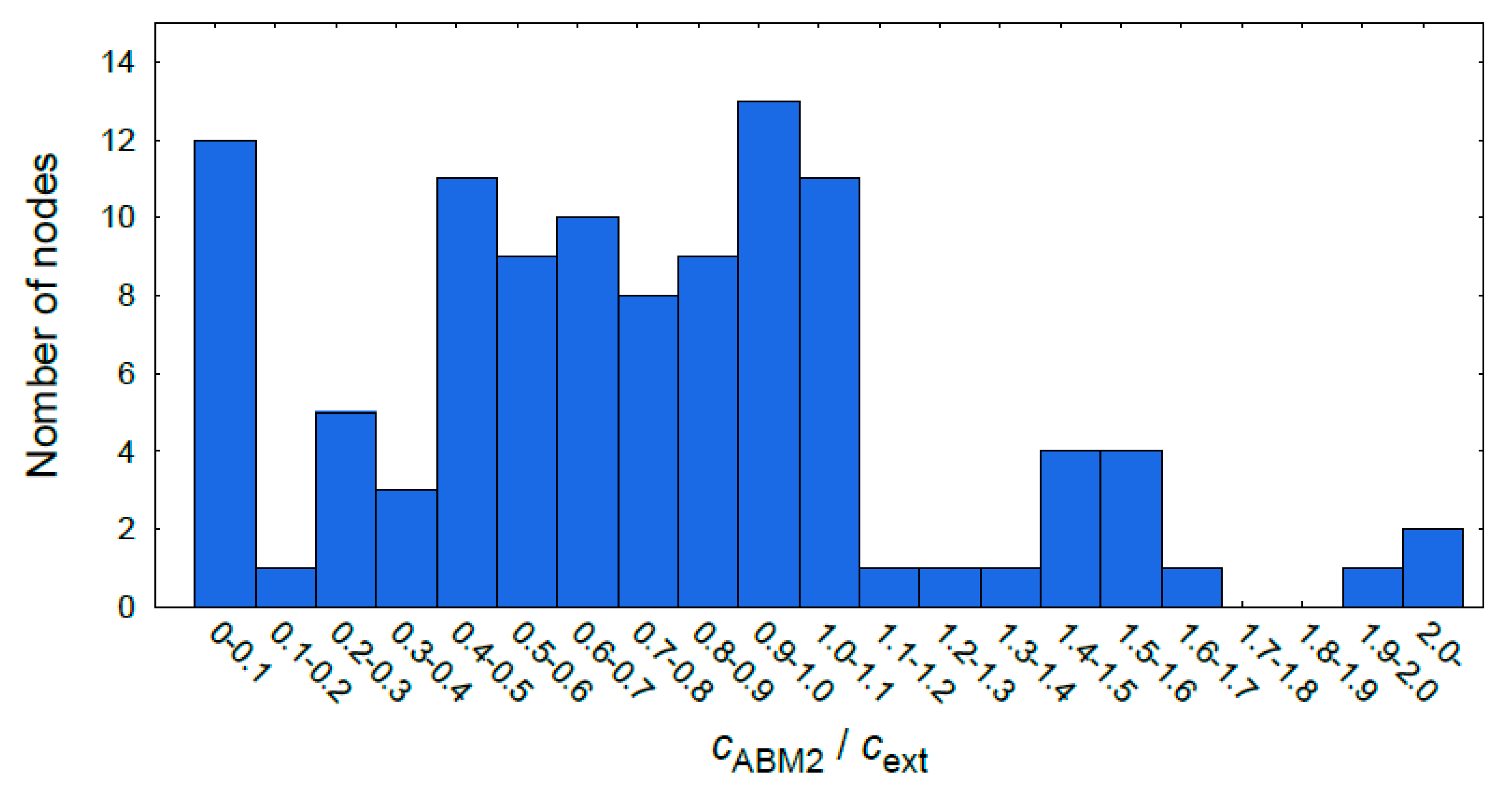
After 4500 simulations, we counted the number of visits to each node and show the results in Figure 7 (the two nodes are not shown): node 11, rickshaw terminal (counts = 179), and node 231, rickshaw stopping primarily for passenger rides (counts = 3196). The distribution of the data points in this numerical result is closer to that in Figure 5 than that in Figure 6. For instance, the noted discrepancies of the counts at nodes 251 and 271 are consistent in both Figure 5 and Figure 7. However, we found several data points that still possess different values as well as some different trends. Figure 8 indicates a histogram about the ratio of the values of agent visits in Figure 7 to those in Figure 5. A fraction of 40% in the total nodes have similar values in both the experimental (Figure 5) and simulation (Figure 7) data with 20% errors, but the data in other nodes are either too small or too large. The real stochastic process observed in the rickshaw mobility is partially in a simple Markov chain, based on memoryless random walks, which corresponds to the fraction of 40% as similar counts at nodes. But other components remain in the higher-order Markov information sources with hysteresis or memories [38], which might create a discrepancy between Figure 5 and Figure 7.
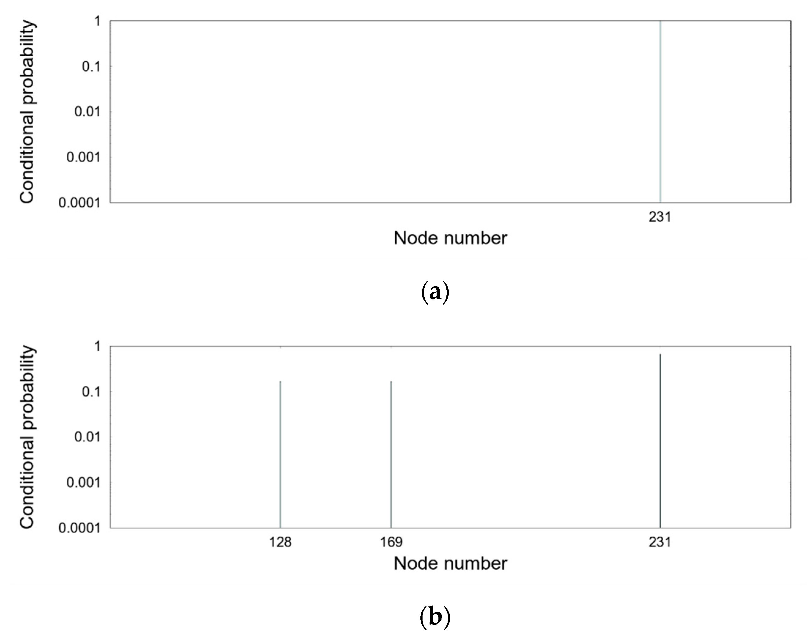
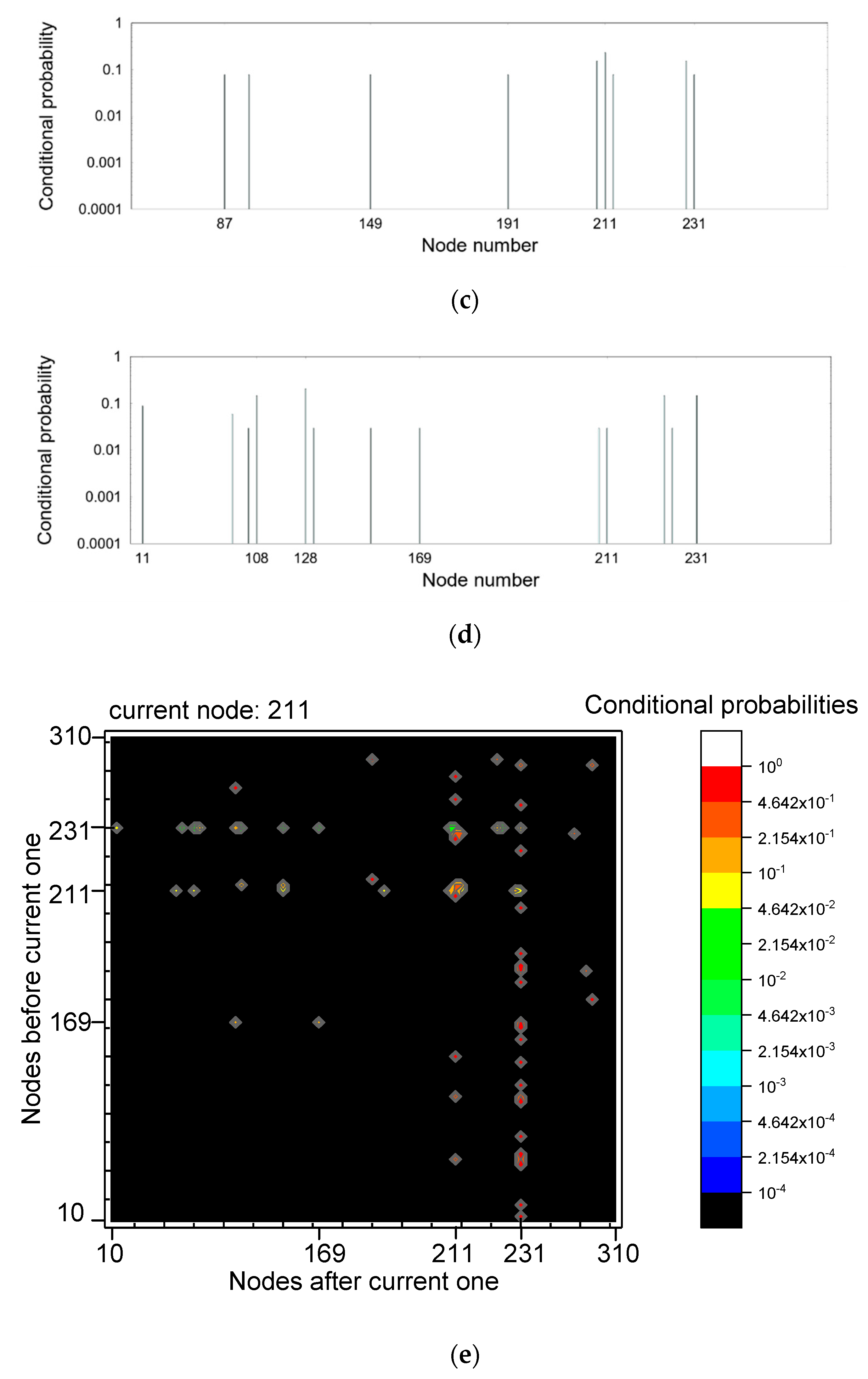
To specifically consider this discrepancy, we examined examples of the details in the total system of mobile probabilities p(ni+1|ni) derived from the datasets on the cloud server. We rearranged the statistical data to perform a closer survey about visits to node ni with the information of node ni−1, the one before node ni, and node ni+1, the one after node ni. Such data are summarized in one matrix for node ni whose column and row denote nodes ni−1 and ni+1. Then, the vector data in one column (corresponding to a fixed ni−1) indicates p(ni+1|ni) where ni+1 is a variable. For instance, at node ni = 211, we compared the probability distribution p(ni+1|ni) in some specific cases for ni−1 (11, 169, 211 and 231) in Figure 9. At node 211, since it is a nearby node of 231, the rickshaw always has large or certain values of p(ni+1|ni) with ni+1 = 231 in all the cases of ni−1. However, among these four cases of ni−1, the probability distributions of p(ni+1|ni) have different spectra components. For instance, if ni−1 = 11, the rickshaw goes to node 231 by node 211, which is out of a simple Markov chain, and moves toward multiple nodes with almost equal probabilities when ni−1 = 231.
Figure 9e shows all the entries in the p(ni+1|ni) matrix. If the rickshaw process were completely random, line profiles parallel to x axis would be the same for all the y values. Some parts of the area are similar, with similar spectra of ni+1, but we found different profiles at other parts, e.g., in the region of 169 < ni+1 < 211. These distinctions indicate bias and/or memory effects that create different components from the random one that we considered in our agent-based simulations. We conclude that there is a certain number of biased routes with fixed sequences in these rickshaw operations.
From pure geographical locations and the individual information of each sightseeing spot, we cannot predict such scheduled routes; a sightseeing guidebook or a powerful social network service message may recommend such routes, or a rickshaw driver might suggest them to passengers. Such conditions strongly depend on the specific situations of each sightseeing area. In other words, by sufficient previous offers of sightseeing information, tourist behaviors by sightseeing vehicles can be biased. In other cases in which each tourist independently selects the sightseeing route, using such an agent-based model and simulation runs we can roughly predict the macroscopic behaviors of time-integrated rickshaw visits to nodes from such simple datasets stored in the cloud server. That is, using the devices and the analysis shown here, one can obtain fractions of tourist behaviors in random components with their own volition, or in biased components by information offered in advance.

4. Conclusions

We designed an electronic device for sightseeing vehicles with data storage on a cloud server and simulated tourist behaviors recorded in cloud datasets in an agent-based model. In the device, GPS and LPWA modules were controlled by a microprocessor that was installed on a rickshaw operated in the Hikone sightseeing area. The device sent location data to the cloud server every five minutes and stored them as visualization in open data for tourists, which are our analysis target. The stored data were visualized, and their location information was matched with graphs with specific topology reflecting a geographical map. Numerical simulations, which were based on an agent-based model in which agents moved along directed edges in the graphs, reproduced a part of the features stored in the cloud datasets: randomness in the stochastic process. This model without memory in a simple Markov chain does not describe another part of the rickshaw features, which may be subjected to data biases, as scheduled visits, induced by various recommendations to tourists as typical sightseeing routes. The fraction of such components depends on specific local situations, but our method allows us to quantitatively estimate such fractions.

Author Contributions

K.Y. constructed the data transfer system, did primary analysis shown here, made the figures, and partially wrote the manuscript. J.Y. and S.M. (Shigeyuki Miyagi) assisted in the construction of the data transfer system. S.M. (Shinsuke Minami) and D.M. designed the LPWA device and arranged the open data project of the rickshaws. O.S. conceived and designed the research activities and wrote the paper. All authors have read and agreed to the published version of the manuscript.

Funding

This study was based on the open data project performed in the GAT Hikone Association in the Hikone Chamber of Commerce and Industry. This study was partially supported by the Regional ICT Research Center for Human, Industry and Future at The University of Shiga Prefecture, and by the Cabinet Office, Government of Japan.

Acknowledgments

All the authors thank the members of the GAT Hikone Association for their useful comments on this study, and also the Hikone-Kirakusha Association for their corporation during the device’s installation on the rickshaws operated in Hikone. The authors (K.Y., S.M. (Shigeyuki Miyagi) and O.S.) thank K. Enomoto and S. Matsuyama at the University of Shiga Prefecture for their useful comments on this study.

Conflicts of Interest

The authors declare no conflict of interest.

Appendix A

We used node numbers to represent geographical positions in this study. The detailed numbering of the nodes, representing each spatial mesh, is shown in Figure A1. We digitized our target area in Hikone using equal-sized, 20 by 20 meshes, and attached sequential numbers to each mesh from the southwest end to the northeast end.
In Figure A1, we put identical sequential numbers from 0 to 399 on the geographical meshes in Hikone’s sightseeing area. In Table A1, we list the identical numbers for the nodes that were visited by a rickshaw at least once. We used these numbers as pointers on the x axis in Figure 9a–d and on the x and y axes in Figure 9e. Since we cannot put all numbers on the axis in Figure 9, the sequence in Table A1 is displayed as a reference. All the others are in the sequence shown below.
Figure A1. Geographical meshes with node numbers for the Hikone sightseeing area used in this study. Size of one grid or one mesh unit is 88.4 by 93.6 m. LN (35.282095 deg.), LS (35.266204 deg.), LE (136.263345 deg.), and LW (136.242744 deg.) indicate area boundary lines defined by corresponding degrees in longitude and latitude.
Electronics 09 00116 g0a1
Table A1. List of identical numbers for nodes visited by a rickshaw at least once.
Sequence on Axes in Figure 9Number in Figure A1 and in Axes of Figure 9Sequence on Axes in Figure 9Number in Figure A1 and in Axes of Figure 9
11044188
21145189
32946190
43047191
53148193
64649194
74750195
84851196
94952197
106753205
116854206
128755207
138856208
149157209
1510758210
1610859211
1710960212
1811061213
1911162214
2011363215
2112764224
2212865225
2312966226
2413067227
2513168229
2614569230
2714670231
2814771232
2914872244
3014973245
3115974246
3216575249
3316676250
3416777251
3516878253
3616979262
3717080264
3817381265
3917782271
4017883273
4117984290
4218585306
4318686310

References

  1. Brockmann, D.; Hufnagel, L.; Geisel, T. The scaling laws of human travel. Nature 2006, 439, 462–465. [Google Scholar] [CrossRef] [PubMed]
  2. Gonzalez, M.C.; Hidalgo, C.; Barabasi, A.-L. Understanding individual human mobility patterns. Nature 2008, 453, 779–782. [Google Scholar] [CrossRef] [PubMed]
  3. Menezes, T.; Roth, C. Natural scales in geographical patterns. Sci. Rep. 2017, 7, 45823. [Google Scholar] [CrossRef] [Green Version]
  4. Sagarra, O.; Szell, M.; Santi, P.; Diaz-Guilera, A.; Ratti, C. Supersampling and network reconstruction of urban mobility. PLoS ONE 2015, 10, e0134508. [Google Scholar] [CrossRef] [Green Version]
  5. Taczanowska, K.; Bielanski, M.; Gonzalez, L.-M.; Garcia-Masso, X.; Toca-Herrera, L.L. Analyzing spatial behavior of backcountry skiers in mountain protected areas combining GPS tracking and graph theory. Symmetry 2017, 9, 317. [Google Scholar] [CrossRef] [Green Version]
  6. Peng, C.; Jin, X.; Wong, K.C.; Shi, M.; Lio, P. Collective human mobility pattern from taxi trips in urban area. PLoS ONE 2012, 7, e34487. [Google Scholar]
  7. Tachet, R.; Sagarra, O.; Santi, P.; Resta, G.; Szell, M.; Strogatz, S.H.; Ratti, C. Scaling law of urban ride sharing. Sci. Rep. 2017, 7, 42868. [Google Scholar] [CrossRef] [Green Version]
  8. Cui, Y.; Zhang, M.; Li, J.; Luo, H.; Zhang, X.; Fu, Z. WSMS: Wearable stress konitoring system based on IoT multi-sensor platform for living sheep transportation. Electronics 2019, 8, 441. [Google Scholar] [CrossRef] [Green Version]
  9. Lucchi, E.; Pereira, L.D.; Andreotti, M.; Malaguti, R.; Cennamo, D.; Calzolari, M.; Frighi, V. Development of a compatible, low cost and high accurate conservation remote sensing technology for the hygrothermal assessment of historic walls. Electronics 2019, 8, 643. [Google Scholar] [CrossRef] [Green Version]
  10. Hossen, M.I.; Michael, G.K.O.; Connie, T.; Lau, S.H.; Hossain, F. Smartphone-based context flow recognition for outdoor parking system with machine learning approaches. Electronics 2019, 8, 784. [Google Scholar] [CrossRef] [Green Version]
  11. Blanco-Claraco, J.L.; Mañas-Alvarez, F.; Torres-Moreno, J.L.; Rodriguez, F.; Gimenez-Fernandez, A. Benchmarking particle filter algorithms for efficient velodyne-based vehicle localization. Sensors 2019, 19, 3155. [Google Scholar] [CrossRef] [Green Version]
  12. Torres, R.; Ohashi, O.; Pessin, G. A machine-learning approach to distinguish passengers and drivers reading while driving. Sensors 2019, 19, 3174. [Google Scholar] [CrossRef] [Green Version]
  13. Vázquez-Diosdado, J.A.; Paul, V.; Ellis, K.A.; Coates, D.; Loomba, R.; Kaler, J. A combined offline and online algorithm for real-time and long-term classification of sheep behaviour: Novel approach for precision livestock farming. Sensors 2019, 19, 3201. [Google Scholar] [CrossRef] [Green Version]
  14. Lima, W.S.; Souto, E.; El-Khatib, K.; Jalali, R.; Gama, J. Human activity recognition using inertial sensors in a smartphone: An overview. Sensors 2019, 19, 3213. [Google Scholar] [CrossRef] [PubMed] [Green Version]
  15. Zhang, J.; Williams, S.; Johnson, H.; Behr, J.; Genrich, J.; Dean, J.; van Domselaar, M.; Agnew, D.; Wyatt, F.; Stark, K.; et al. Southern California permanent GPS geodetic array: Continuous measurements of regional crustal deformation between the 1992 Landers and 1994 Northridge earthquakes. J. Geophys. Res. 1997, 102, 18013–18033. [Google Scholar]
  16. Gleason, S.; Gebre-egiabher, D. GNSS Applications and Methods; Artech House: Norwood, MA, USA, 2009. [Google Scholar]
  17. Jin, S.; Feng, G.P.; Gleason, S. Remote sensing using GNSS signals: Current status and future directions. Adv. Space Res. 2011, 47, 1645–1653. [Google Scholar] [CrossRef]
  18. Choi, W.; Chang, Y.-S.; Jung, Y.; Song, J. Low-power LoRa signal-based outdoor positioning using fingerprint algorithm. ISPRS Int. J. Geo-Inf. 2018, 7, 440. [Google Scholar] [CrossRef] [Green Version]
  19. Ogudo, K.A.; Nestor, D.M.J.; Khalaf, O.I.; Kasmaei, H.D. A device performance and data analytics concept for smartphones’ IoT services and machine-type communication in cellular networks. Symmetry 2019, 11, 593. [Google Scholar] [CrossRef] [Green Version]
  20. Tian, H.; Weitnauer, M.A.; Nyengele, G. Optimized gateway placement for interference cancellation in transmit-only LPWA networks. Sensors 2018, 18, 3884. [Google Scholar] [CrossRef] [Green Version]
  21. Gershenfeld, N.; Krikorian, R.; Cohen, D. The internet of things. Sci. Am. 2004, 291, 76–81. [Google Scholar] [CrossRef]
  22. Kranz, M.; Holleis, P.; Schmidt, A. Embedded interaction: Interacting with the internet of things. IEEE Internet Comput. 2010, 14, 46–53. [Google Scholar] [CrossRef] [Green Version]
  23. Atzori, L.; Iera, A.; Morabito, G. The Internet of Things: A Survey. Comput. Netw. 2010, 54, 2787–2805. [Google Scholar] [CrossRef]
  24. Tokognon, C.J.A.; Gao, B.; Tian, G.Y.; Yan, Y. Structural health monitoring framework based on Internet of Things: A survey. IEEE Internet Things J. 2017, 4, 619–635. [Google Scholar] [CrossRef]
  25. Statistical Data of Visiting Tourists in Shiga Prefecture in 2018 (Tentative Version). Available online: https://www.pref.shiga.lg.jp/kensei/tokei/syougyou/302905/303923.html (accessed on 21 October 2019). (In Japanese).
  26. Sen, J. The Sha Fu of Calcutta: The past, the present], and the future of the hand-rickshaw pullers of Calcutta. Is a civilized and progressive transition possible? Bull. Concerned Asian Sch. 1998, 30, 37–49. [Google Scholar] [CrossRef]
  27. Naomi, W.J. Rickshaw runner. South. Rev. 2007, 43, 326. [Google Scholar]
  28. Eubank, S.; Guclu, H.; Kumar, V.S.A.; Marathe, M.V.; Srinivasan, A.; Toroczkai, Z.; Wang, N. Modelling disease outbreaks in realistic urban social networks. Nature 2004, 429, 180. [Google Scholar] [CrossRef]
  29. Miyashita, K. Incremental design of perishable goods markets through multi-agent simulations. Appl. Sci. 2017, 7, 1300. [Google Scholar] [CrossRef] [Green Version]
  30. Lozano, Á.; De Paz, J.; Villarrubia González, G.; Iglesia, D.; Bajo, J. Multi-agent system for demand prediction and trip visualization in bike sharing systems. Appl. Sci. 2018, 8, 67. [Google Scholar] [CrossRef] [Green Version]
  31. Mariani, S.; Omicini, A. Special issue “multi-agent systems”: Editorial. Appl. Sci. 2019, 9, 954. [Google Scholar] [CrossRef] [Green Version]
  32. Julian, V.; Botti, V. Multi-agent systems. Appl. Sci. 2019, 9, 1402. [Google Scholar] [CrossRef] [Green Version]
  33. Nishikawa, K. The castle town of Hikone and its future. Ekistics 2006, 73, 436–441. [Google Scholar]
  34. Hokone Travel Guide. Available online: https://visit.hikoneshi.com/en/ (accessed on 21 October 2019).
  35. Sigfox, a 0G Network. Available online: https://www.sigfox.com/en (accessed on 21 October 2019).
  36. Hikone Kirakusha Rickshaw. Available online: https://visit.hikoneshi.com/en/plan_your_visit/activities/hikone-kirakusha-rickshaw/ (accessed on 21 October 2019).
  37. How about “Jinriki-Sha,” Japanese Traditional Taxi by a Self-Running Driver? Available online: https://www.gat-hikone.net/rikisha/index.php (accessed on 21 October 2019).
  38. Cover, T.M.; Thomas, J.A. Elements of Information Theory, 2nd ed.; John Wiley & Sons: Hoboken, NJ, USA, 2006; pp. 52–59. [Google Scholar]
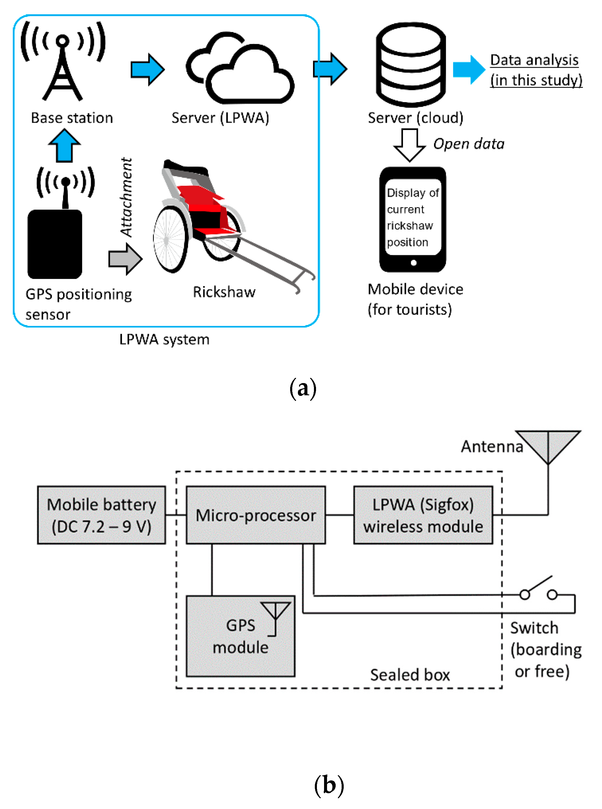
Figure 1. System and device designed for detecting and accumulating rickshaw spatiotemporal data. (a) System with signal flows from rickshaw to tourists. Current rickshaw position is open data from internet. (b) Configuration of GPS positioning sensor with electronic modules.
Electronics 09 00116 g001
Figure 2. Information displayed in mobile device shown in Figure 1a [37]. Rickshaw location shown in red is visible on the geographical map as open data on the internet. Detailed geographical meshes used in this study are shown in the Appendix (Figure A1). LN (35.282095 deg.), LS (35.266204 deg.), LE (136.263345 deg.), and LW (136.242744 deg.) indicate area boundary lines for data analysis, defined by corresponding degrees in longitude and latitude.
Electronics 09 00116 g002
Figure 3. Typical example of time evolution of rickshaw velocity, based on raw data shown in Table 1: speed or velocity is calculated by assuming paths with straight line distance between two sequential pair values of longitude and latitude.
Electronics 09 00116 g003
Figure 4. Graph with specific topology corresponding to the geographic map in the Hikone sightseeing area. Identical numbers in nodes correspond to those of meshes in Figure 2.
Electronics 09 00116 g004
Figure 5. Distributions of rickshaw visits based on all accumulated data recorded on cloud server in our survey period. We eliminated two nodes since counts at these two points are excessive: node 11 (counts = 693) and node 231 (counts = 3293).
Electronics 09 00116 g005
Figure 6. Distributions of agent visits based on agent-model simulations. Agents are mobile in network with graph topology shown in Figure 4. We removed two nodes since the counts at these two points have more values than the others: node 11 (counts = 50) and node 231 (counts = 3554).
Electronics 09 00116 g006
Figure 7. Distributions of agent visits based on agent-model simulations. Agents are mobile in a network with 86 nodes with 594 directed edges (not shown), configured with conditioning probabilities derived from datasets of real rickshaws on the cloud server. We removed two nodes since the counts at these two points have more values than the others: node 11 (counts = 179) and node 231 (counts = 3196).
Electronics 09 00116 g007
Figure 8. Histogram of nodes as a function of ratio for number of agent visits in Figure 7 to that of rickshaw visits in Figure 5. A total of 86 nodes were visited by rickshaw recorded and used here.
Electronics 09 00116 g008
Figure 9. Conditional probabilities p(ni+1|ni) from node 211 to other typical nodes: (a) Case with previous visiting node 11. (b) Case with previous visiting node 169. (c) Case with previous visiting node 211. (d) Case with previous visiting node 231. (e) Contour plots of matrix entries of conditional probabilities p(ni+1|ni) for ni = 211. x and y axes indicate ni+1 and ni−1. Sequence in (bd) along x axis for nodes after current one (211) in (e) along x and y axes is listed in Table A1.
Electronics 09 00116 g009aElectronics 09 00116 g009b
Table 1. Examples of rickshaw datasets detected by our electronic device and stored in cloud server.
Device 1TimeLatitudeLongitudeNode #Passenger
741D8216:00:05 on 9 May 201935.272357136.252577149Y
741D8216:05:04 on 9 May 201935.272905136.250573167Y
741D8216:10:04 on 9 May 201935.272558136.250197147Y
741D8216:15:04 on 9 May 201935.272575136.250168167Y
741D8216:20:05 on 9 May 201935.272557136.250228147Y
741D8216:25:05 on 9 May 201935.272105136.252340149Y
741D8216:30:05 on 9 May 201935.272092136.254260231Y
741D8216:35:04 on 9 May 201935.275110136.254282231Y
741D8216:40:05 on 9 May 201935.275143136.254302231Y
741D8216:45:05 on 9 May 201935.275102136.254227231Y
741D8216:48:52 on 9 May 201935.275095136.254198231N
741D8216:50:05 on 9 May 201935.275085136.254213231N
741D8216:55:05 on 9 May 201935.272402136.252560149N
741D8217:00:05 on 9 May 201935.268890136.25157768N
741D8217:05:05 on 9 May 201935.266640136.25431811N
741D8217:10:04 on 9 May 201935.266535136.25443211N
741D8217:15:05 on 9 May 201935.266890136.25440011N
741D8217:20:05 on 9 May 201935.266762136.25447511N
741D8217:25:05 on 9 May 201935.266733136.25452511N
741D8217:30:05 on 9 May 201935.266713136.25446511N
1 Since numbering of devices installed to rickshaws is identical, we can recognize corresponding rickshaw.