Article

Low-Complexity Failed Element Diagnosis for Radar-Communication mmWave Antenna Array with Low SNR

1
ZNDY of Ministerial Key Laboratory, School of Mechanical Engineering, Nanjing University of Science and Technology, Nanjing 210094, China
2
North Information Control Research Academy Group Co., Ltd., Nanjing 211153, China
3
Key Laboratory of Digital TV System of Guangdong Province and Shenzhen City, Research Institute of Tsinghua University in Shenzhen, Shenzhen 518057, China
4
Research Institute of Tsinghua, Pearl River Delta, Guangzhou 510530, China
5
Beijing National Research Center for Information Science and Technology (BNRist), Beijing 100084, China
6
Laboratory of Array and Information Processing, Hohai University, Nanjing 210098, China
*
Authors to whom correspondence should be addressed.
Electronics 2019, 8(8), 904; https://doi.org/10.3390/electronics8080904
Submission received: 1 July 2019 / Revised: 6 August 2019 / Accepted: 8 August 2019 / Published: 15 August 2019
(This article belongs to the Section Microwave and Wireless Communications)

Abstract

:
The millimeter-wave (mmWave) antenna array plays an important role in the excellent performance of wireless sensors networks (WSN) or unmanned aerial vehicle (UAV) clusters. However, the array elements are easily damaged in its harsh working environment but hard to be repaired or exchanged timely, resulting in a serious decline in the beamforming performance. Thus, accurate self-diagnosis of the failed elements is of great importance. In previous studies, there are still significant difficulties for large-scale arrays under extremely low SNR. In this paper, a diagnosis algorithm with low complexity and high reliability for the failed elements is proposed, which is based on a joint decision of communication signal and sensing echoes. Compared with the previous studies, the complexity of the algorithm is reduced by the construction of low-dimensional feature vectors for classification, the decoupling of the degree of arrival (DOA) estimation and the failed pattern diagnosis, with the help of the sub-array division. Simulation results show that, under an ultra-low SNR of −12.5 dB for communication signals and −16 dB for sensing echoes, an accurate self-diagnosis with a block error rate lower than 8% can be realized. The study in this paper will effectively promote the long-term and reliable operation of the mmWave antenna array in WSN, UAV clusters and other similar fields.

1. Introduction

In recent years, millimeter-wave (mmWave) antenna arrays have been widely studied and applied in the field of communication [1] and radar [2] devices, due to their small size and ease of large-scale integration. Especially in the field of wireless sensors network (WSN) [3,4,5,6] and unmanned aerial vehicle (UAV) cluster [7,8], the miniaturized mmWave antenna array effectively reduces the total volume as well as power consumption, and increases the working life. Considering the harsh environment, such as battlefields and wilderness, failure of the array elements cannot be avoided, and will do great harm to the performance of both the function of radar and communication, as shown in Figure 1. However, the antenna array is inconvenient to be repaired or exchanged timely. Thus, the self-diagnosis of the failed elements is the key to ensure its robust performance.
Each of the failed element patterns can be regarded as a “mode”, so that multiple classification algorithms based on machine learning can be used for array diagnosis. Xu et al. [9] pioneered the diagnosis of failed elements based on support vector machine (SVM) [10], and Yeo et al. [11] studied the choice of kernel function and improved the accuracy of the diagnosis. However, these methods construct feature vectors based on the radiation pattern of the antenna, and suppose that the degree of arrival (DOA) of the received signal is perpendicular to the antenna array. These methods can be applied only in very limited and idealized situations, and can hardly be used in practice, because the sensors/UAVs simultaneously receives multiple signals from different unknown directions. To solve this problem, Wang et al. [12] proposed a new method for constructing feature vectors. It is based on the autocorrelation matrix constructed by the received signals with the known DOAs, and is suitable for multiple signals arriving simultaneously. However, under ultra-low signal-to-noise ratio (SNR), it is difficult to get an accurate DOA at the first estimation, especially with the unknown array failures.
In recent years, to further improve the integration of smart sensors/UAVs, joint radar-communication technology has emerged. The joint system realizes environment sensing and communication simultaneously in one device, especially via the same antenna array [13,14,15,16,17]. Therefore, the information fusion of radar and communication provides a new way to diagnose the failed array elements at low SNR, as the adaptive algorithm we have proposed in previous research [16]. The received communication signals and the sensing echoes are used to construct the autocorrelation matrix for diagnosis, respectively, and the two estimation results are selected according to two confidence factors which measure the credibility of the communication signal and the sensing echoes, the details of the joint radar-communication system is shown in the Supplementary Material, Note S2. As a result, accurate array element diagnosis is achieved even at a low SNR. However, the diagnosis algorithm relies on a feature vector with M 2 dimension (M is the length of each sub-array), and an iterative process of DOA estimation, SVM model training and failed array diagnosis should be performed. Such a relatively high complexity makes it hard to be applied for large-scale antenna arrays in mmWave.
Therefore, an array diagnosis algorithm at ultra-low SNR with low complexity and high reliability is still a challenging and practical issue for WSN/UAV cluster, which is the inspiration for this work. This paper proposes a new diagnosis algorithm, which reduces the computational complexity from two aspects without affecting the diagnosis accuracy. Firstly, with a division of sub-arrays, the DOA is accurately estimated by information fusion and statistical inference, so that the decoupling between the failed pattern diagnosis and the DOA estimation is realized. Secondly, a new feature vector is constructed with only M dimension, and a correction algorithm is proposed to promote the accuracy. Overall, this paper realizes the diagnosis of failed array elements with low complexity and high accuracy, and provides support for the long-term application of WSN/UAV clusters equipped with large-scale mmWave antenna arrays in ultra-low SNR environment.

2. System Model

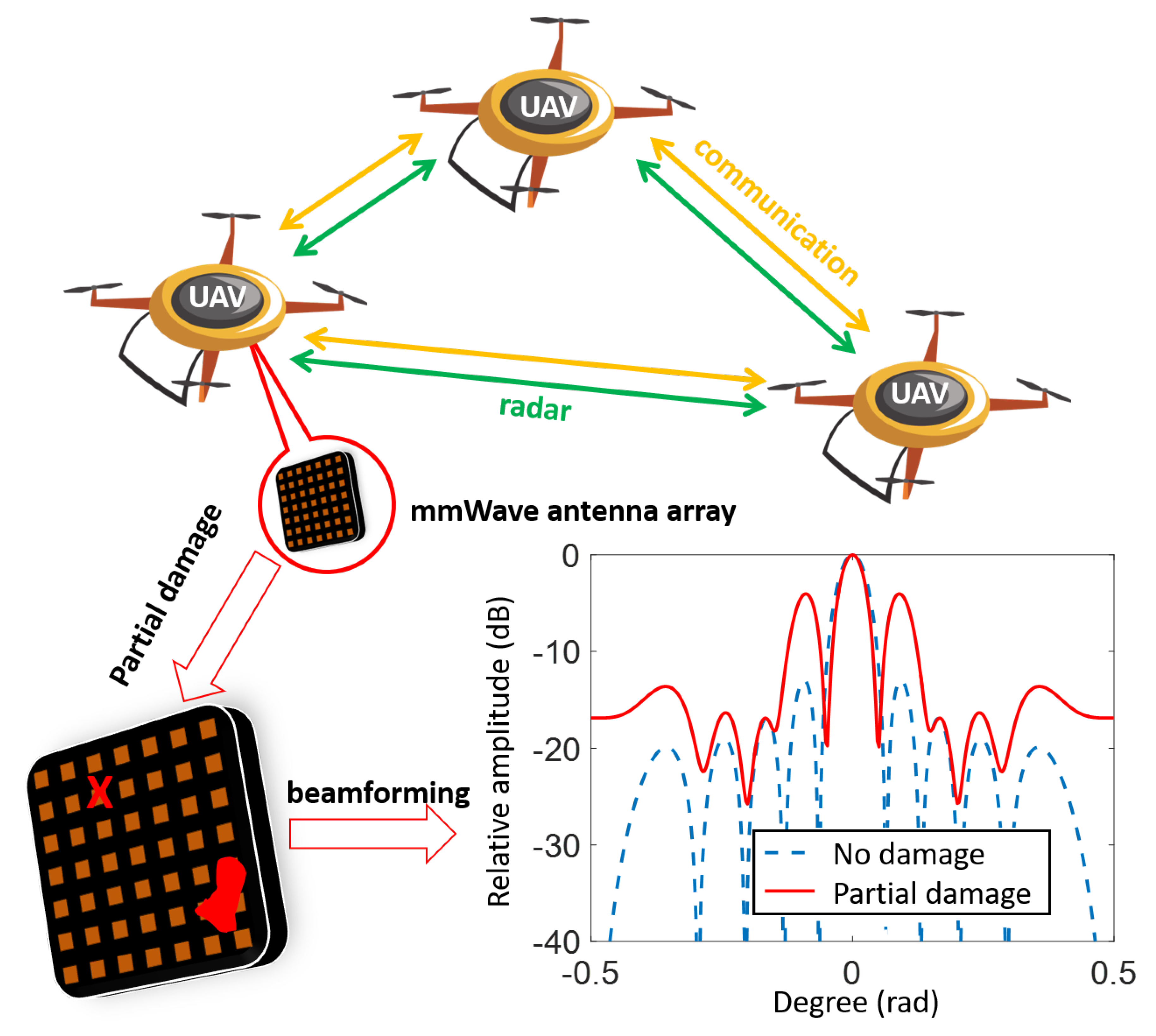
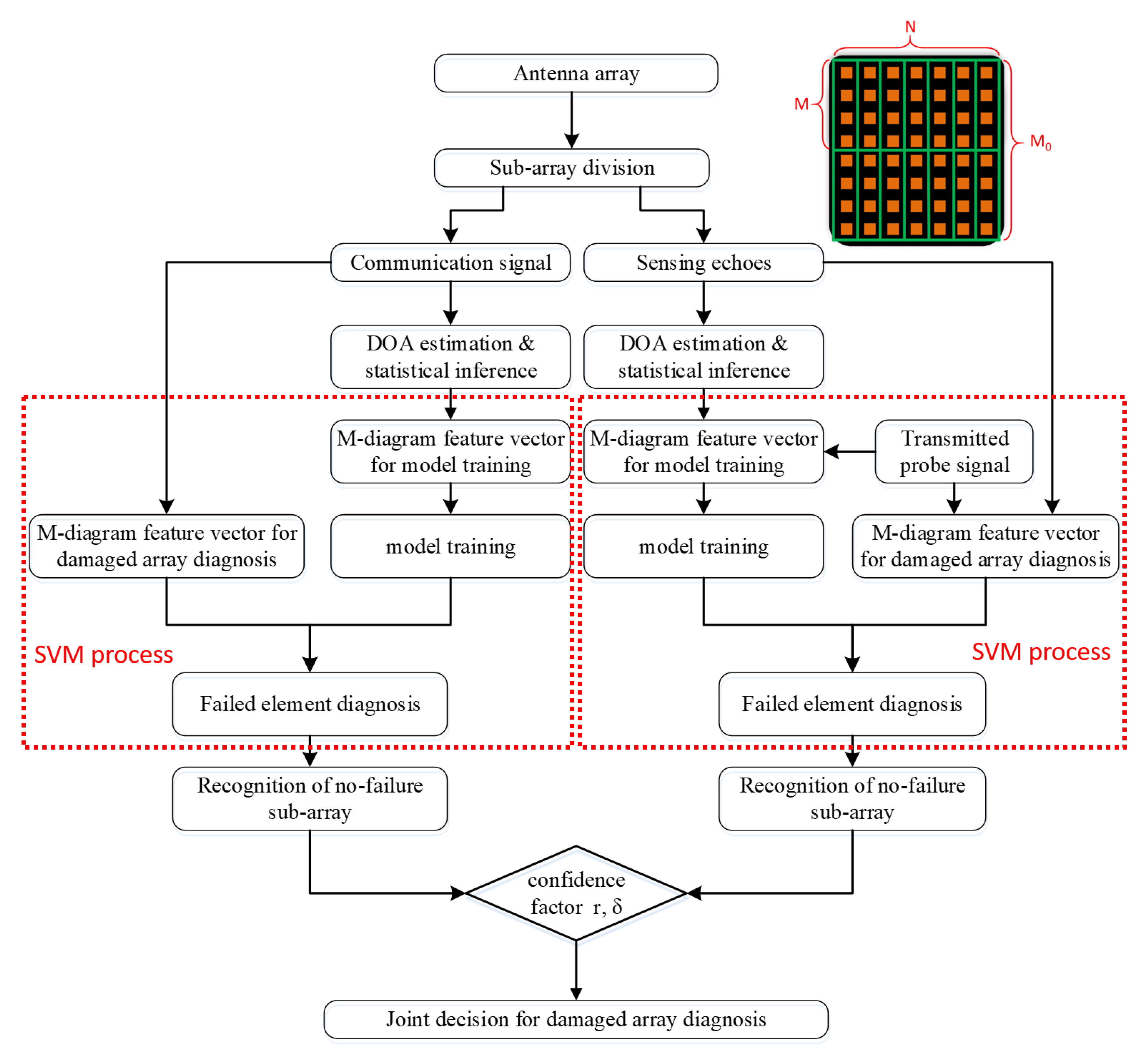
2.1. Joint Diagnosis Based on Radar-Communication System

The core idea of joint diagnosis is summarized as follows. Firstly, the antenna array of M 0 · N elements is divided into sub-arrays of M · 1 , and the number of all the sub-arrays is P n · N (where P n = M 0 / M ), as shown in the upper-right of Figure 2. Then, based on the sub-arrays, the diagnosis of the failed array elements is performed with the communication signal and the sensing echoes, respectively, including DOA estimation and failed pattern estimation based on SVM. Finally, the reliability of the diagnosis results is evaluated by two confidence factors, and the more reliable one is selected as the final diagnosis. The whole diagram of the algorithm is shown in Figure 2, and the details of the joint diagnosis algorithm is shown in the Supplementary Material, Note S1.
It is true that the diagnosis can be achieved based on either the communication signals or the sensing echoes separately. Considering a harsh environment where the SNR is extremely low, the estimation accuracy based solely on communication signals or sensing echoes is not high enough. Thanks to the joint radar-communication system, the antenna array will receive both the communication signals as well as the sensing echoes at the same time, so that the joint diagnosis can be carried out without extra implementation. Since the communication signals and the sensing echoes are independent, the possibility that both of them are with huge noise at the same time is not high, so the diagnosis accuracy can be improved through adaptive decision.
The diagnosis based on the communication signal and the sensing echoes are adaptively selected according to two confidence factors for higher reliability of the joint diagnosis.
The first confidence factor is based on the belief that a reliable diagnosis is usually obtained at a high SNR, and is defined as the relative SNR between the communication signals and sensing echoes,
r = SNR c SNR r
where SNR c and SNR r are the estimated SNR after beamforming based on the estimated DOA and failed pattern.
The second confidence factor is based on the belief that reliable diagnosis based on the sensing echoes is usually obtained under accurate DOA estimation, and is defined as the variance of the selected DOA estimation from sub-arrays for final decision of DOA,
δ = avg ( ( θ 0 ( : , C ) - θ est ) 2 )
where avg() means the average of all the elements in the vector. θ 0 is an array of all the sub-array DOA estimation results, where the L s elements corresponds to the angle of the L s sources, and each row is corresponding to one sub-array. C is the set selected to calculate θ est . θ 0 ( : , C ) means the rows corresponding to C with all the columns.
These two confidence factors reflect the quality of the received signals, and result in a “double security”. Some more details are presented in Supplementary Material, Note S4. The diagnosis based on sensing echoes is adopted only if the two confidence factors are lower than the thresholds. Thus, the final decision of the diagnosis is,
d est = d r , r < r th , δ < δ th d c , e l s e
where d r is the diagnosis based on sensing echoes, d c is based on communication signals, with details in the Supplementary Material, Note S3, and r th and δ th are the thresholds of confidence factor r and δ , respectively.

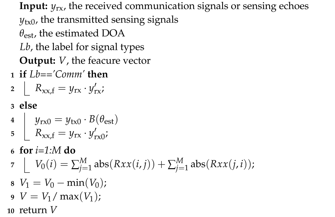
2.2. M-Dimensional Classification Vector for SVM

Feature extraction is extremely critical for machine learning algorithms [18,19], and SVM algorithms are no exception. In this paper, to characterize the failure pattern of the sub-array, the feature vectors are constructed based on the received signals of each array element as well as the estimated DOAs. Since the dimension of the feature vector for the SVM algorithm has a significant impact on the computational complexity, a M-dimensional feature vector is designed, which is summarized in Algorithm 1. Compared with the previous work based on a feature vector of M 2 dimension [16], the complexity is significantly reduced.
It is supposed that the received signals from the failed elements only contain noises, so that the failed pattern will be reflected on the correlation array R xx ,
R xx = Y rx · Y r x
where Y rx is the received signal.
When the ith element is failed, the corresponding row and column of R xx will only contain noise. Therefore, the sum of each row and column of R xx will reflect the failed elements,
V 0 ( i ) = j = 1 M abs ( R xx ( i , j ) ) + j = 1 M abs ( R xx ( j , i ) )
When the ith element is failed, V 0 ( i ) will be a small value which only contains the power of noises. Considering the surroundings with large noise, a normalized stretching process is proposed,
V = ( V 0 min ( V 0 ) ) / max ( V 0 min ( V 0 ) )
Therefore, based on the M-dimensional feature vector V proposed above, failure diagnosis can be carried out based on communication signals or sensing echoes.
Further, the transmitted sensing signals are known to the device, so that the received sensing echoes can be reconstructed with the estimated DOA,
y rx 0 = y tx 0 · B ( θ est )
where y tx 0 is the transmitted symbols for sensing, θ est is the estimated DOA, and B ( θ est ) is the array composed of steering vectors.
Since information of the sensing signal is known, the effects of noise can be partially eliminated, which will help to improve the diagnosis of the failure pattern. From this perspective, the correlation array R xx is replaced by cross-correlation between the reconstructed sensing echoes y rx 0 and the received sensing echoes y rx ,
R xx , f = y rx · y rx 0
Algorithm 1: M-diagram feature vector.
Electronics 08 00904 i001

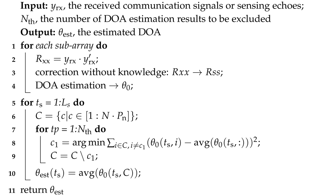
2.3. Accurate Estimation of DOA Based on Statistical Analysis

As analyzed in Section 2.2, DOA estimation has an important impact on the reconstruction of the received sensing echoes. In addition, for model training, all the failed patterns should be traversed, and the training set is composed of the randomly constructed received signal based on the estimated DOA. In all, DOA plays an important part in the diagnosis algorithm, and must be accurately estimated.
Thanks to the division of sub-arrays, an accurate estimation of DOA based on statistical analysis is proposed, as summarized in Algorithm 2.
For a single sub-array, the commonly used MUSIC algorithm [20,21] is applied based on the correlation array,
R xx = Y rx · Y r x
where Y rx is the received signal.
When the ith element fails, the corresponding row and column of R xx will only contain noise, so that the SVD decomposition of the matrix will be significantly affected. On the other hand, when there is no noise, the values on the same diagonal from lower left to upper right are equal. As a result, the element with the largest absolute value on the same diagonal in R xx is most likely to be a normal element without failure. For any ( M 1 ) t M 1 , t Z , R xx is adjusted to R ss ,
R ss ( p , p + t ) = max { R xx ( p , p + t ) | p [ 1 , M ] , p + t [ 1 , M ] }
Then, eigenvalue decomposition is performed on R ss . The eigenvalues are ranked in descending order as { γ 1 , , γ M } , and the corresponding eigenvector is { v 1 , , v M } . Thus, the estimated DOA vector θ 0 is corresponding to the first L s peaks of the estimation vector of spatial spectrum,
P est ( θ ) = 1 ( b H ( θ ) E n E n H b ( θ ) )
where E n = [ v L s + 1 , , v M ] , and b ( θ k ) = [ e j 0 , e j 2 π / ν d sin θ k , , e j 2 π / ν d ( M 1 ) sin θ k ] is the steering vector.
However, such a DOA estimation is likely to be with large errors in low SNR, which is the key issue hindering the application of past literature [9,10,11,12] in low SNR environments, unless with iteration of DOA estimation and failed elements diagnosis [16]. In this paper, based on the DOA estimation results of all the sub-arrays, more accurate DOA estimation can be realized through statistically analysis. Therefore, no iteration is needed during diagnosis, and the computation complexity can be reduced.
The estimation results obtained from each sub-array constitute a matrix of θ 0 . To get a more accurate estimation result, the P n · N N th ones with the highest reliability are selected as set C. For the t s th source of degree, the selected ones minimize the variance of θ 0 ( t s , C ) in all the possible choice,
C = arg min ( θ 0 ( t s , C ) a v g ( θ 0 ( t s , C ) ) ) 2 , C a r d ( C ) = P n · N N th
where Card( ) represents the number of elements in the set.
The estimated DOA of the t s th source is the average of the selected ones,
θ est ( t s ) = avg ( θ 0 ( t s , C ) )
Algorithm 2: DOA estimation and statistical inference.
Electronics 08 00904 i002

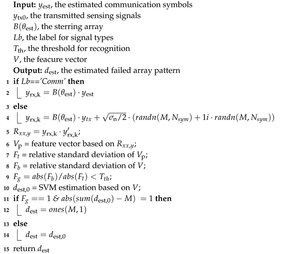
2.4. Recognition of No-Failure Subarray

The feature vectors constructed in this paper significantly decrease the computational complexity of SVM, compared to M 2 -dimensional vectors. At the same time, the loss in diagnosis performance is also unavoidable due to information loss through signal processing.
The performance loss mainly exists in the difficulty to identify the no-failure sub-array. After the normalized stretching process in Algorithm 1, the fluctuation of the feature vector is enlarged, which has different effects on the sub-array with failed elements and the no-failure sub-array. On the one hand, for a sub-array with failed elements, it is beneficial to combat the influence of noise and highlight the effect of the failed elements on the feature vector, improving the accuracy of the diagnosis. As shown in Figure 3a, the lower bound of the feature vector without stretching process is as high as 0.6, which is likely to be regarded as fluctuation of the no-failure sub-array. After the stretching process, it is very close to the feature vector without noise, so that the failed elements of No. 4 and No. 5 can be recognized more easily. On the other hand, for a sub-array without failed elements, the feature vector will be randomly stretched according to its maximal and minimal value, so that it may be randomly confused with any failure pattern. As shown in Figure 3b, the feature vector of a no-failure sub-array is stretched and is likely to be confused with the sub-array whose elements of No. 5 and No. 6 have failed. In other words, with the proposed normalized stretching process in the construction of low-dimensional feature vectors, the random error will be amplified, so that it is easy to be randomly confused with some other failure mode.
To solve this problem, a special SVM-independent recognition algorithm is designed for the no-failure sub-array to avoid performance loss caused by the dimension reduction of the feature vector, which is summarized in Algorithm 3. The core idea of the algorithm is that the fluctuation rate of the feature vector increases as the number of failed elements increases.
The fluctuation rate of the feature vector F b is defined as,
F b = abs Var ( V ) V / M
Suppose the sub-array has no failed elements, and mark the corresponding fluctuation rate as F t . The no-failure sub-array is decided when F b / F t < T th and the diagnosis result d est , 0 shows there is more than one failed element in the sub-array based on V. In this case, the estimated failed pattern is corrected to no-failure.
d est = ones ( M , 1 ) , F b / F t < T th , d est , 0 < M 1 d est , 0 , e l s e
where ones() means a M-dimension vector with all the M elements are equal to 1.
The corresponding fluctuation rate of the no-failure sub-array F t is defined as,
F t = V a r ( V p ) V p / M
where V p is the reconstructed feature vector based on R xx , y according to Algorithm 1, and R xx , y is defined as,
R xx , y = y rx , k · y rx , k
where y rx , k is the reconstructed received signal of the no-failure sub-array. For communication signals, it is reconstructed with the decoded communication symbols y est ,
y rx , k = B c ( θ est ) · y est
while, for sensing echoes, it is reconstructed with the known transmitted symbols and the estimated noise power σ n
y rx , k = B ( θ est ) · y t x + σ n / 2 · ( randn ( M , N s y m ) + 1 i · randn ( M , N s y m ) )
where randn() means a random array with each element in Gaussian distribution.
Algorithm 3: No-failure sub-array recognition.
Electronics 08 00904 i003

3. Results and Discussion

The effectiveness of the proposed algorithm under ultra-low SNR was verified and the performance gain was analyzed through simulation. The diagnosis algorithm was applied on antenna arrays of the scales of 10 × 10/20 × 20/30 × 30/40 × 40. The noise added to communication signals was modeled as the additive white Gaussian noise, and the average SNR was marked as SNR c . For the sensing echoes, to reflect its greater randomness, the SNR itself was modeled as Gaussian distribution, with the average of SNR rm and the variance of σ rs 2 . In the following simulation, unless specially stated, it was set that SNR c = −12.5 dB, SNR rm = −16 dB, σ rs 2 = 7. In the no-failure sub-array recognition algorithm, T th was set as 1.5 for communication signals and 2 for sensing echoes. In DOA estimation, N th was set as 3/4 P n · N .

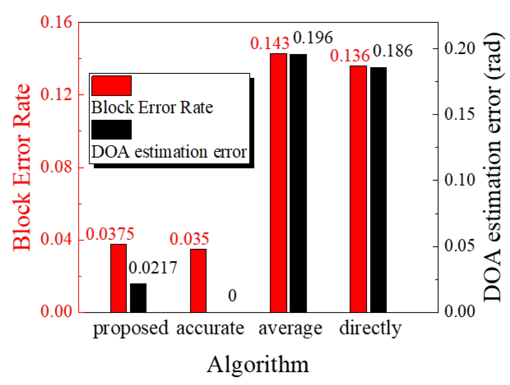
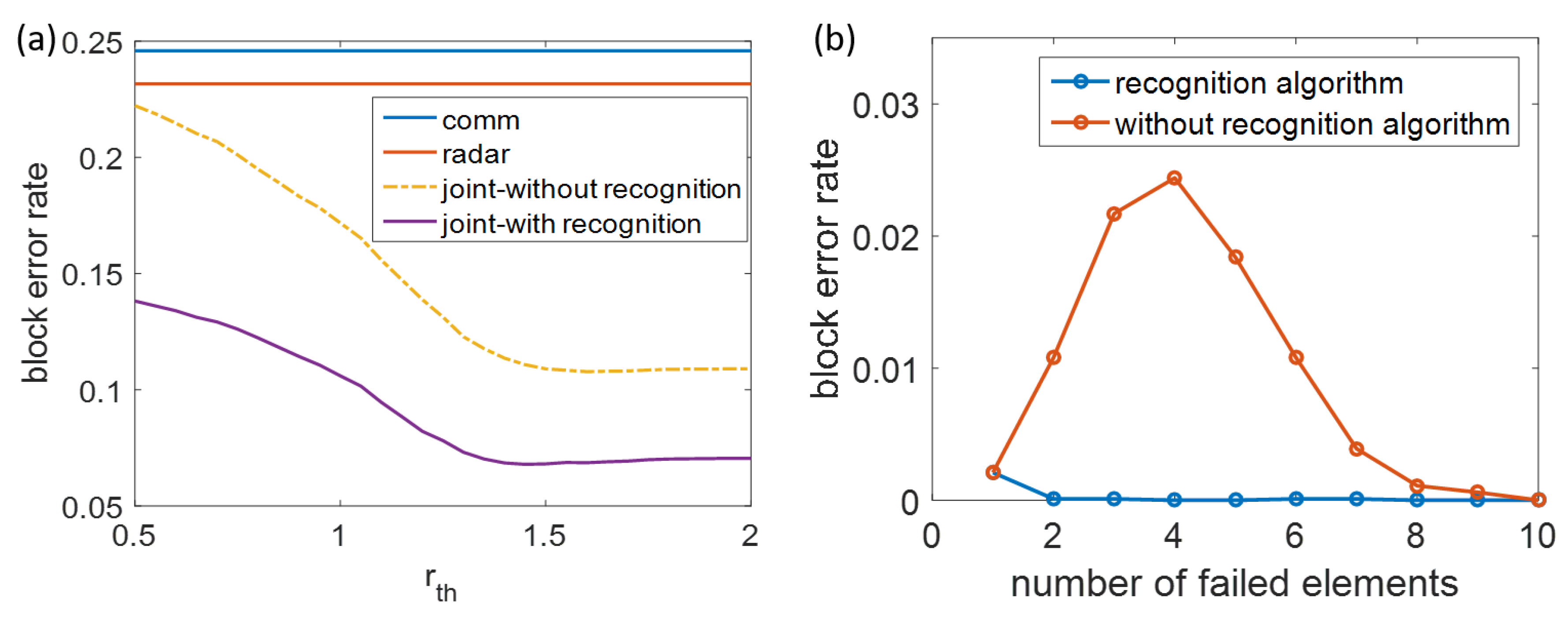
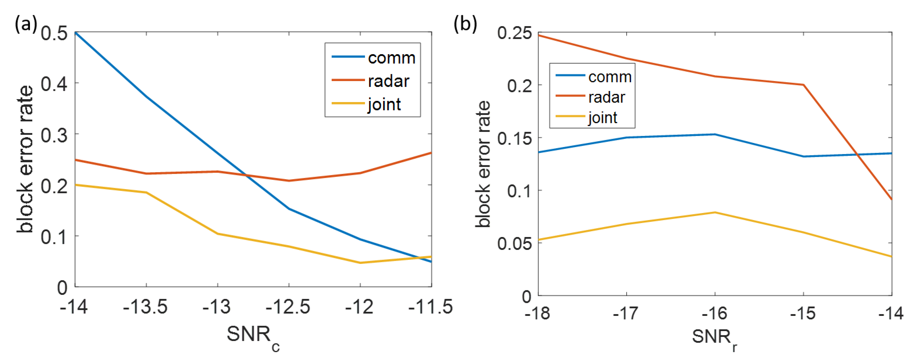
3.1. Accuracy of the Diagnosis

The accuracy of the diagnosis was measured by the block error rate, which is the ratio of misjudged sub-arrays in all sub-arrays. As shown in Figure 4, the block error rate of the joint diagnosis performed on a 10 × 10 antenna array is always lower than that of the single diagnosis based on communication signals or sensing echoes, no matter how the confidence factors δ th and r th are set. Especially, with suitable confidence factors (when r th is around 1.5 and δ th is around 0.02), the block error rate is lower than 8%, which is about 1/2 of that based on the single diagnosis of communication signals, and about 1/3 of that based on the single diagnosis of sensing echoes.
Further, the effectiveness of the proposed algorithm was validated with four antenna arrays of different scales, and the threshold of two confidence factors were also scanned.
As shown in Figure 5, firstly, for all four arrays, the block error rate is lower than 8% under such a low SNR. Secondly, for the two confidence factors, there is a “wide bottom” around the optimal threshold ( r th [ 1.4 , 2 ] , δ th [ 0.02 , 0.04 ] ), which means that, when the threshold of the confidence factor is not particularly far from the optimal value, the block error rate can be maintained at a low level close to that under the optimal threshold. This “wide bottom” is particularly important for practical application of WSN/UAV clusters, because it is difficult to accurately estimate the optimal threshold of the confidence factors in harsh environments. Thirdly, when the scale of arrays increases, e.g., from 10 × 10 to 40 × 40, the block error rate continues to decrease slowly. In other words, the application of large-scale mmWave MIMO antenna arrays will also benefit the diagnosis accuracy.
The gain of joint diagnosis is essentially obtained from the information fusion of communication signal and sensing echoes, and is influenced by the threshold of the two confidence factors. When δ th is set as 0.02, as r th increases, joint diagnosis is not likely to trust the diagnosis based on communication signal unless it is much more credible compared with the sensing echoes. Further analysis is as follows. There are two sources of the selected communication signals. One (marked as [C1]) is the relatively higher SNR of communication signals, meaning that r > r th . Another (marked as [C2]) is the relatively poorer DOA estimation of the sensing echoes, meaning that δ > δ th . When r th raises from low value to its optimal value, the ratio of the selected communication signal drops significantly, which is the combined effect of the rapid decline of [C1] and the slow rise of [C2], as shown in Figure 6a. The essence of this change is that a significant proportion of communication signal with actually relatively low SNR in [C1] originally is discarded, as shown in Figure 6b, so that the average SNR and accuracy of diagnosis based on the communication signal and the joint diagnosis are significantly improved. However, while the r th is larger than its optimal value and continues to raise, the ratio of [C1] gradually drops to zero, and the selected communication signals are mainly from [C2], which has a relatively low and widely distributed SNR. Although the SNR of [C2] also increases as r th increases (Figure 6c), the gain is not sufficient to compensate for the decreased ratio of [C1] (Figure 6d). In total, the accuracy of diagnosis based on communication signals and the joint diagnosis begins to decrease slowly. The above mechanism makes r th have an optimal value around 1.5, as shown in Figure 5a.
Similar to r th , δ th also has an optimal value. When r th is set as 1.5, as δ th increases, the joint diagnosis is more likely to trust the diagnosis based on sensing echoes. As shown in Figure 7a, the selected ratio of the sensing echoes will increase gradually. From the perspective of δ th , the diagnosis is ranked in the order of its credibility, from the most credible to the least credible one. As δ th increases, the median and distribution of SNR of the selected sensing echoes become smaller (Figure 7b). When δ th is very small, the signal quality requirement for sensing echoes is too strict, and some estimation results with better accuracy than that of communication signals are also excluded. As δ th increases, more diagnosis with higher accuracy based on sensing echoes are selected, and thus the overall diagnosis accuracy improves. However, when the δ th is beyond its optimal value and continues to increase, the selected sensing echoes continue to increase, and more and more sensing echoes with relatively low diagnosis accuracy are selected, making the block error rate of joint diagnosis start to rise. The above mechanism makes δ th have an optimal value near 0.02, as shown in Figure 5b.

3.2. Algorithm Complexity Analysis

Compared with previous research [16], this paper significantly reduces the complexity from three aspects. The first is from the SVM algorithm itself, the second is from the SVM classifier’s iterative training, and the third is from sub-array division. The detailed analysis is as follows, and the effectiveness of the compensation algorithm was validated through simulation.
First, take the Bunch–Kaufman training algorithm as an example. The typical computational complexity of SVM model training is [22],
O ( N sv 3 + L N sv 2 + d L N sv ) O ( d L 2 )
where N sv is the number of support vectors, L is the number of training set, and d is the dimension of each sample.
In previous research [16], the dimension of feature vector is M 2 , so that the complexity is,
O ( N sv 3 + L N sv 2 + M 2 L N sv ) O ( M 2 L 2 )
while, in this paper, the dimension of each sample is reduced from M 2 to M, so that the complexity is reduced to,
O ( N sv 3 + L N sv 2 + M L N sv ) O ( M L 2 )
Inevitably, the reduction of the feature vector dimension affects the accuracy of model training and estimation. To solve this problem, in this paper, Algorithm 3 is proposed for a secondary check of the diagnosis results. The algorithm aims at the misjudgement that is most likely to occur, where the no-failure sub-array is misjudged as there are failed array elements.
As shown in Figure 8a, with the recognition algorithm, the block error rate is decreased from about 11% to 7%. With the optimal threshold r th = 1.5, the block error rate of which the no-failure sub-array is misjudged as partially failed sub-array, is shown in Figure 8b. Apart from the misjudgement that a no-failure sub-array is misjudged as that of one failed element, almost all other misjudgments are corrected by the recognition algorithm. The simulation validated that the no-failure recognition algorithm is effective, and the reduction of feature vectors’ dimension only brings little loss of performance.
Secondly, since the accuracy of DOA estimation based on a single sub-array is poor, especially when there is no knowledge of failed array elements, in previous studies [16], an iterative DOA estimation and failed array diagnosis algorithm was applied. However, each iteration requires retraining of the classifier, and the complexity grows linearly with the number of iterations. In this paper, based on the DOA estimation results of multiple sub-arrays, the information fusion is carried out by means of statistical inference. As a result, a more accurate DOA can be obtained first based on Algorithm 2, and some iterations are avoided.
The effect of the improved DOA accuracy obtained by statistical interference based on the estimated DOAs by each sub-array is shown in Figure 9, where r th = 1.5 and δ th = 0.02. The block error rate based on the estimated DOAs by the proposed statistical analysis algorithm is as low as 3.75%, which is only 1.07 times the block error rate based on the accurate DOAs. Compared with the results based on the DOAs of one single subarray or the average of all sub-arrays, the block error rate based on the proposed algorithm is less than 30% of theirs. This significant improvement in block error rate is indeed due to the improved accuracy of DOA estimation. As shown in Figure 9, the DOA estimation error by the proposed statistical analysis algorithm is only about 0.0217 rad, about 10% of the DOA estimation error by single subarray or average of all subarrays. These simulation results validate that, with the statistical inference of DOA estimation, decoupling the DOA estimation and failure array element diagnosis can be achieved with almost no loss of performance.
Thirdly, since the antenna array of size M 0 · N is divided into sub-arrays of M · 1 and accurate DOA estimation is achieved, the model training is only needed for one time with the scale of M · 1 . Therefore, the number of support vectors N sv and the number of training sets L would not increase as the scale of antenna array grows. Further, more sub-arrays also contribute to more accurate DOA estimation.

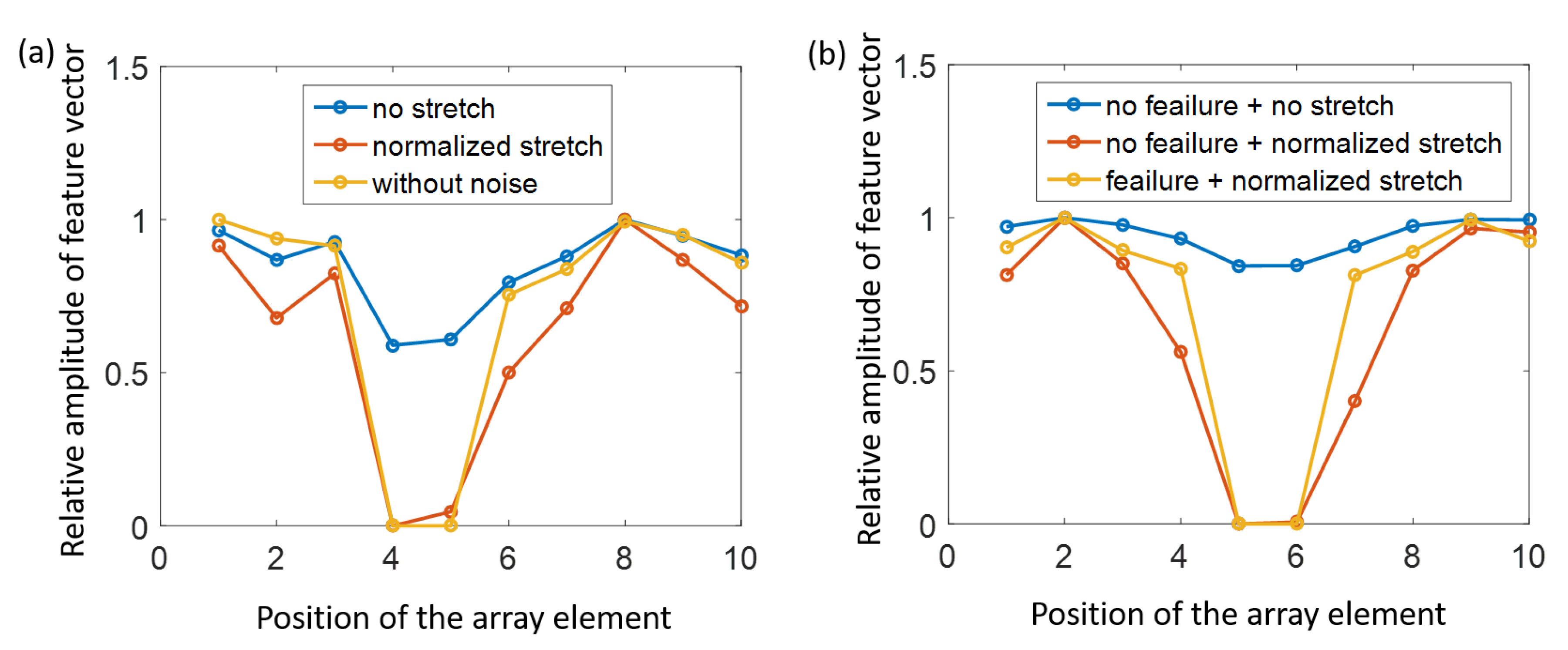
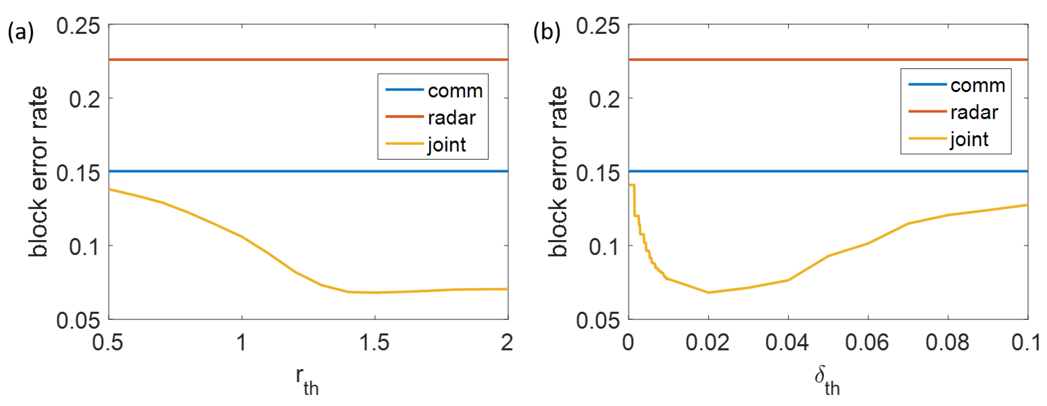
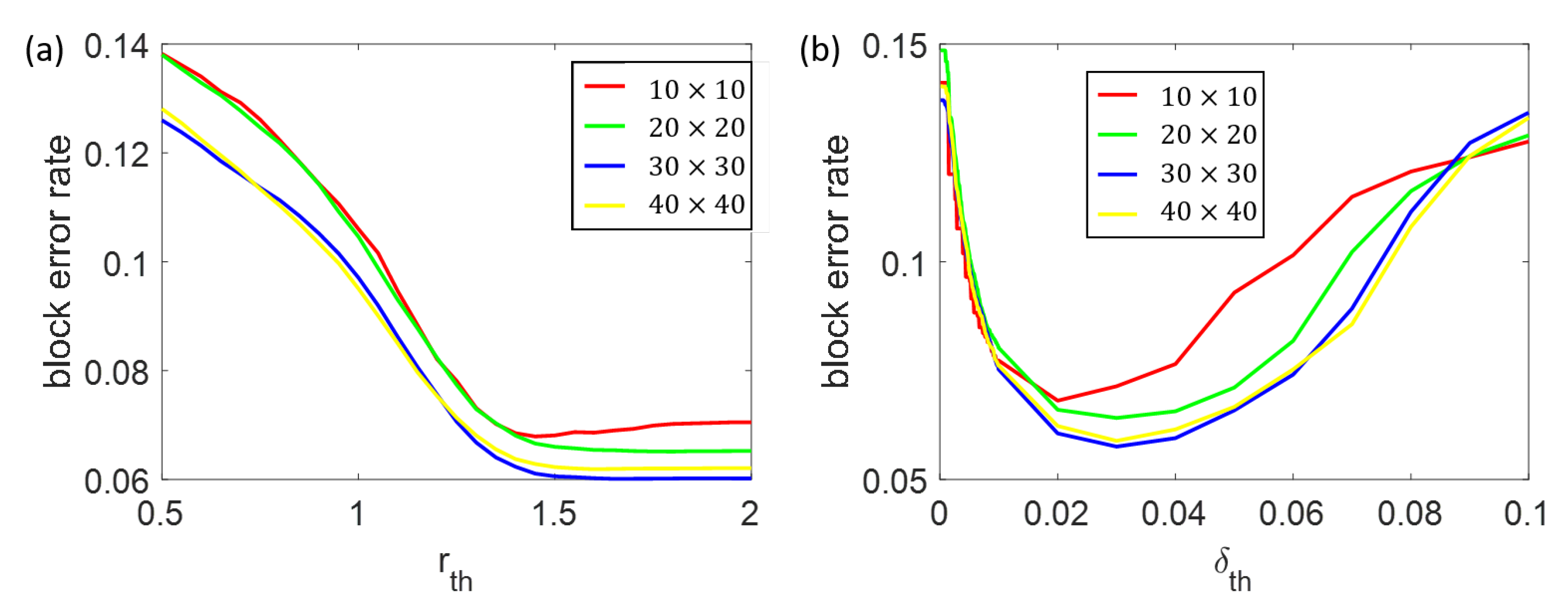
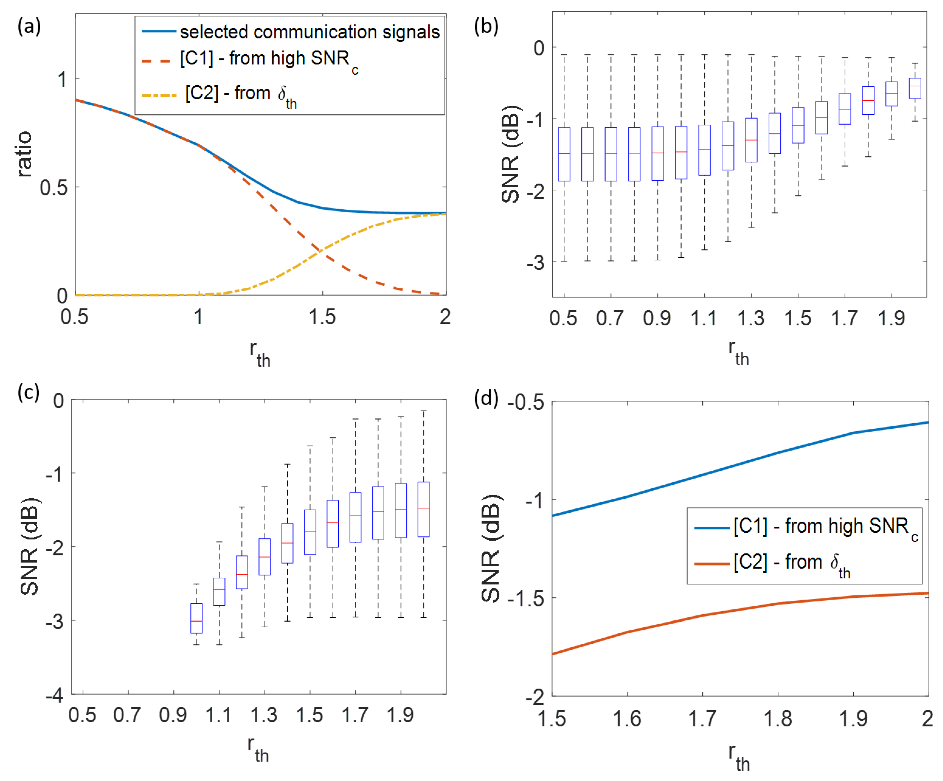
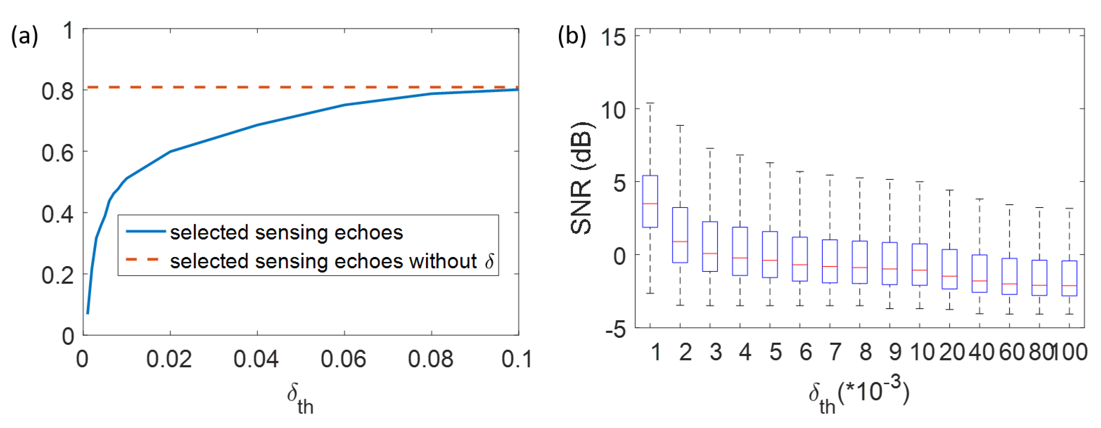
3.3. Robustness of Environmental Parameters

Finally, the robustness of the joint diagnosis was studied. In practical applications, the most unstable environmental parameter is the SNR of the communication signals and sensing echoes. Fortunately, as shown in Figure 10, by fixing r th = 1.5, δ th = 0.02, and scanning the SNR of the communication signal from −14 dB to −11.5 dB, or the average SNR of the sensing echoes from −18 dB to −14 dB, the joint diagnosis can always achieve significant performance gain compared to the single diagnosis based on communication signals or sensing echoes. Therefore, the robustness of the joint diagnosis algorithm and the feasibility of its practical application were verified.

3.4. Discussion of Performance

The above simulation analysis further demonstrates the superiority of the proposed algorithm, namely high accuracy, low complexity and strong environmental robustness. The high accuracy comes from information fusion of the communication signal and the sensing echo. The low complexity comes from the low-dimensional feature vectors, the division of sub-arrays, an accurate DOA estimation, and thus the non-iterative architecture. Strong environmental robustness ensures that the algorithm can perform well in a large range of SNR.
The core of the joint algorithm is information fusion of the communication signal and the sensing echo. In most cases, the quality of the two will not be particularly poor at the same time, so that performance gain will be obtained through joint processing. In a few extreme cases, when the quality of both is particularly poor, the performance of the proposed algorithm is not as superior as in ordinary situations, and still needs to be improved in further study.

4. Conclusions

To achieve self-diagnosis of the large-scale mmWave antenna array of WSN/UAV clusters, a joint diagnosis algorithm based on the information fusion of communication signals and sensing echoes is proposed, achieving high accuracy and low complexity. The normalized stretching process of the feature vector, the accurate estimation of DOA based on statistical analysis, and the recognition of no-failure sub-array helps promote the diagnosis accuracy, which is always lower than 8% at an ultra-low SNR of −12.5 dB for communication signals and −16 dB for sensing echoes. The complexity is reduced from a design of M-dimensional feature, the decoupling of DOA estimation and failed element diagnosis, and the division of the large-scale antenna array. The performance is robust within a wide range of SNR, and is insensitive to the threshold of confidence factors. This study will promote the practical application of WSN/UAV clusters with mmWave antenna array.

Supplementary Materials

The following are available online at https://www.mdpi.com/2079-9292/8/8/904/s1.

Author Contributions

Q.L. and K.D. proposed the idea; Q.L., K.D. and Y.Z. conceived and designed the experiments; Q.L., K.D. and X.W. performed the experiments; Q.L. and K.D. analyzed the data; H.Z. and D.J. contributed analysis tools; and Q.L. wrote the paper.

Funding

This work is supported in part by the Central University Special Funding for Basic Scientific Research under Grant No. 309171B8805 and 30918012201, and in part by National Natural Science Foundation of China under Grant No. 91738202 and 61790553, and in part by Shenzhen science and technology plan projects under Grant No. JCYJ20180306170614484.

Conflicts of Interest

The authors declare no conflict of interest. The founding sponsors had no role in the design of the study; in the collection, analyses, or interpretation of data; in the writing of the manuscript, and in the decision to publish the results.

Abbreviations

The following abbreviations are used in this manuscript:
WSNwireless sensors networks
UAVunmanned aerial vehicle
SVMsupport vector machine
DOAdegree of arrival

References

  1. Niu, Y.; Li, Y.; Jin, D.; Su, L.; Vasilakos, A.V. A survey of millimeter wave communications (mmWave) for 5G: opportunities and challenges. Wirel. Netw. 2015, 21, 2657–2676. [Google Scholar] [CrossRef]
  2. Patole, S.M.; Torlak, M.; Wang, D.; Ali, M. Automotive radars: A review of signal processing techniques. IEEE Signal Process. Mag. 2017, 34, 22–35. [Google Scholar] [CrossRef]
  3. Hao, G.; Matters-Kammerer, M.; Milosevic, D.; Baltus, P.G.M. System Analysis of mm-Wave Wireless Sensor Networks; Springer International Publishing: Cham, Switzerland, 2018; pp. 13–19. [Google Scholar]
  4. Qi, N.; Dai, K.; Yi, F.; Wang, X.; You, Z.; Zhao, J. An Adaptive Energy Management Strategy to Extend Battery Lifetime of Solar Powered Wireless Sensor Nodes. IEEE Access 2019, 7, 88289–88300. [Google Scholar] [CrossRef]
  5. Li, Y.; Jin, D.; Su, L.; Zeng, L.; Rashvand, H.F. Performance evaluation of routing schemes for energy-constrained delay/fault-tolerant mobile sensor network. IET wirel. sens. syst. 2012, 2, 262–271. [Google Scholar] [CrossRef]
  6. Zhang, W.; Dong, Y.; Tan, Y.; Zhang, M.; Qian, X.; Wang, X. Electric power self-supply module for WSN sensor node based on MEMS vibration energy harvester. Micromachines 2018, 9, 161. [Google Scholar] [CrossRef] [PubMed]
  7. Sheng, G.; Min, M.; Xiao, L.; Liu, S. Reinforcement Learning-Based Control for Unmanned Aerial Vehicles. J. Commun. Inf. Netw. 2018, 3, 39–48. [Google Scholar] [CrossRef]
  8. Xiao, Z.; Xia, P.; Xia, X. Enabling UAV cellular with millimeter-wave communication: potentials and approaches. IEEE Commun. Mag. 2016, 54, 66–73. [Google Scholar] [CrossRef]
  9. Xu, N.; Christodoulou, C.; Barbin, S.; Martinez-Ramon, M. Detecting failure of antenna array elements using machine learning optimization. In Proceedings of the IEEE Antennas and Propagation Society International Symposium Conference, Honolulu, HI, USA, 9–15 June 2007; pp. 5753–5756. [Google Scholar]
  10. Suthaharan, S. Support vector machine. In Machine Learning Models and Algorithms for Big Data Classification; Springer: Boston, MA, USA, 2016; pp. 207–235. [Google Scholar]
  11. Yeo, B.K.; Lu, Y. Expeditious diagnosis of linear array failure using support vector machine with low-degree polynomial kernel. IET Microw. Antennas Propag. 2012, 6, 1473–1480. [Google Scholar]
  12. Zhu, C.; Wang, W.Q.; Chen, H.; So, H.C. Impaired sensor diagnosis, beamforming, and doa estimation with difference co-array processing. IEEE Sens. J. 2015, 15, 3773–3780. [Google Scholar] [CrossRef]
  13. Nowak, M.; Wicks, M.; Zhang, Z.; Wu, Z. Co-Designed Radar-Communication Using Linear Frequency Modulation Waveform. IEEE Aerosp. Electron. Syst. Mag. 2016, 31, 28–35. [Google Scholar] [CrossRef]
  14. Hassanien, A.; Amin, M.G.; Zhang, Y.D.; Ahmad, F. Dual-Function Radar-Communications: Information Embedding Using Sidelobe Control and Waveform Diversity. IEEE Trans. Signal Process. 2016, 64, 2168–2181. [Google Scholar] [CrossRef]
  15. Zhang, Y.; Li, Q.; Huang, L.; Dai, K.; Song, J. Optimal Design of Cascade LDPC-CPM System Based on Bionic Swarm Optimization Algorithm. IEEE Trans. Broadcast. 2018, 64, 762–770. [Google Scholar] [CrossRef]
  16. Li, Q.; Zhang, Y.; Dai, K.; Huang, L.; Pan, C.; Song, J. An Adaptive Diagnose Scheme for Integrated Radar-Communication Antenna Array with Huge Noise. IEEE Access 2018, 6, 25785–25796. [Google Scholar] [CrossRef]
  17. Li, Q.; Dai, K.; Zhang, Y.; Zhang, H. Integrated Waveform for a Joint Radar-Communication System with High-Speed Transmission. IEEE Wirel. Commun. Lett. 2019. [Google Scholar] [CrossRef]
  18. Zhang, P.; Wang, X.; Chen, J.; You, W.; Zhang, W. Spectral and Temporal Feature Learning with Two-Stream Neural Networks for Mental Workload Assessment. IEEE Trans. Neural Syst. Rehabil. Eng. 2019, 27, 1149–1159. [Google Scholar] [CrossRef] [PubMed]
  19. Zhang, P.; Wang, X.; Zhang, W.; Chen, J. Learning Spatial–Spectral–Temporal EEG Features With Recurrent 3D Convolutional Neural Networks for Cross-Task Mental Workload Assessment. IEEE Trans. Neural Syst. Rehabil. Eng. 2018, 27, 31–42. [Google Scholar] [CrossRef] [PubMed]
  20. Belouchrani, A.; Amin, M.G. Time-Frequency MUSIC. IEEE Signal Process. Lett. 1999, 6, 109–110. [Google Scholar] [CrossRef]
  21. Kundu, D. Modified MUSIC Algorithm for Estimating DOA of Signals. Signal Proces. 1996, 48, 85–90. [Google Scholar] [CrossRef]
  22. Burges, C.J. A tutorial on support vector machines for pattern recognition. Data Min. Knowl. Discov. 1998, 2, 121–167. [Google Scholar] [CrossRef]
Figure 1. Diagram of joint radar-communication system for UAV clusters and the influence of the failed array elements. The graph in the lower right corner is the comparison of the antenna pattern with or without the failed element. The x-axis indicates the direction of the incoming signal, and the y-axis indicates the relative gain of the antenna.
Electronics 08 00904 g001
Figure 2. Diagram of the joint diagnosis algorithm based on radar-communication system and the division of sub-arrays.
Electronics 08 00904 g002
Figure 3. The feature vector with and without normalized stretching. The x-axis is corresponding to the location of each element in the sub-array, and the y-axis is the relative amplitude of feature vector. (a) The vector corresponding to a sub-array with the failed elements of No. 4 and No. 5. (b) The vector corresponding to a no-failure sub-array and a sub-array with the failed elements of No. 5 and No. 6.
Electronics 08 00904 g003
Figure 4. Accuracy comparison of the joint diagnosis algorithm and the single algorithm based on communication signals or sensing echoes: (a) with the scan of r th ; and (b) with the scan of δ th .
Electronics 08 00904 g004
Figure 5. Block error rate of the joint diagnosis algorithm under different array scales: (a) with the scan of r th ; and (b) with the scan of δ th .
Electronics 08 00904 g005
Figure 6. Analysis of confidence factor threshold r th : (a) selected ratio of communication signals; (b) distribution of SNR of [C1] (the selected communication signals due to high SNR c ); (c) distribution of SNR of [C2] (the selected communication signals due to large δ ); and (d) average of SNR of [C1] and [C2].
Electronics 08 00904 g006
Figure 7. Analysis of confidence factor threshold δ th : (a) selected ratio of sensing echoes (where the dotted line indicates the proportion of selected sensing echoes only regardless of the confidence factor δ ); and (b) SNR distribution of the selected sensing echoes
Electronics 08 00904 g007
Figure 8. Analysis of the no-failure recognition: (a) block error rate of the joint diagnosis with and without no-failure recognition; and (b) the ratio of the no-failure sub-array misjudged as failed elements is significantly reduced with the no-failure recognition algorithm.
Electronics 08 00904 g008
Figure 9. Block error rate (in red) and DOA estimation error (in black) with different algorithms: “proposed” corresponds to the proposed DOA estimation algorithm in this paper; “accurate” corresponds to the simulation with accurate DOA; “average” takes the average DOA of all the sub-arrays as the estimated DOA in simulation; and “directly” takes the DOA estimation of each sub-arrays as the estimated DOA in simulation.
Electronics 08 00904 g009
Figure 10. Robustness of the joint diagnosis algorithm: (a) bock error rate with joint and single diagnosis under different SNR c ; and (b) block error rate with joint and single diagnosis under different SNR rm .
Electronics 08 00904 g010

