Optimized Proportional-Integral-Derivative Controller for Upper Limb Rehabilitation Robot

Abstract

This paper proposes a nature inspired, meta-heuristic optimization technique to tune a proportional-integral-derivative (PID) controller for a robotic arm exoskeleton RAX-1. The RAX-1 is a two-degrees-of-freedom (2-DOFs) upper limb rehabilitation robotic system comprising two joints to facilitate shoulder joint movements. The conventional tuning of PID controllers using Ziegler-Nichols produces large overshoots which is not desirable for rehabilitation applications. To address this issue, nature inspired algorithms have recently been proposed to improve the performance of PID controllers. In this study, a 2-DOF PID control system is optimized offline using particle swarm optimization (PSO) and artificial bee colony (ABC). To validate the effectiveness of the proposed ABC-PID method, several simulations were carried out comparing the ABC-PID controller with the PSO-PID and a classical PID controller tuned using the Zeigler-Nichols method. Various investigations, such as determining system performance with respect to maximum overshoot, rise and settling time and using maximum sensitivity function under disturbance, were carried out. The results of the investigations show that the ABC-PID is more robust and outperforms other tuning techniques, and demonstrate the effective response of the proposed technique for a robotic manipulator. Furthermore, the ABC-PID controller is implemented on the hardware setup of RAX-1 and the response during exercise showed minute overshoot with lower rise and settling times compared to PSO and Zeigler-Nichols-based controllers.

1. Introduction

The life expectancy of people, and hence, the number of older adults, is increasing. Elderly people are most vulnerable to strokes. Stroke is among the main causes of limb disabilities and can be fatal [1,2]. According to statistics [3], more than 10 million people suffer from a stroke annually. Consequently, patients become dependent on others for their basic life activities. Physical therapy under the supervision of physiotherapists can help stroke patients to restore the functionality of their disabled limbs. However, traditional physical therapy involves manpower and is highly expensive as the number of patients increases. Rehabilitation robots have been introduced recently to reduce the burden on physiotherapists and increase the number of exercises performed during a therapy session. These robots can provide a more reliable service as they do not face monotony and fatigue failures due to the repetitive nature of the exercises. One of the most widely used control mechanisms employed in such robots is a proportional–integral–derivative (PID) controller. This mechanism is famous for its simple structure and robust performance in a wide range of operating conditions [4]. However, it is quite difficult to select and determine the PID controller parameters for the system. The control parameters are tuned to achieve stable closed-loop response of the system and reach desired positions within a certain time. Several approaches have been proposed to optimize the PID controller parameters, such as Zeigler-Nichols, a classical method to tune PID control parameters [5], fuzzy logic controller [6,7] and evolutionary algorithms such as genetic algorithm (GA) [8], and swarm optimization algorithms such as ant colony algorithm (ACO) [9], particle swarm optimization (PSO) [10] and artificial bee colony (ABC) algorithm [11].

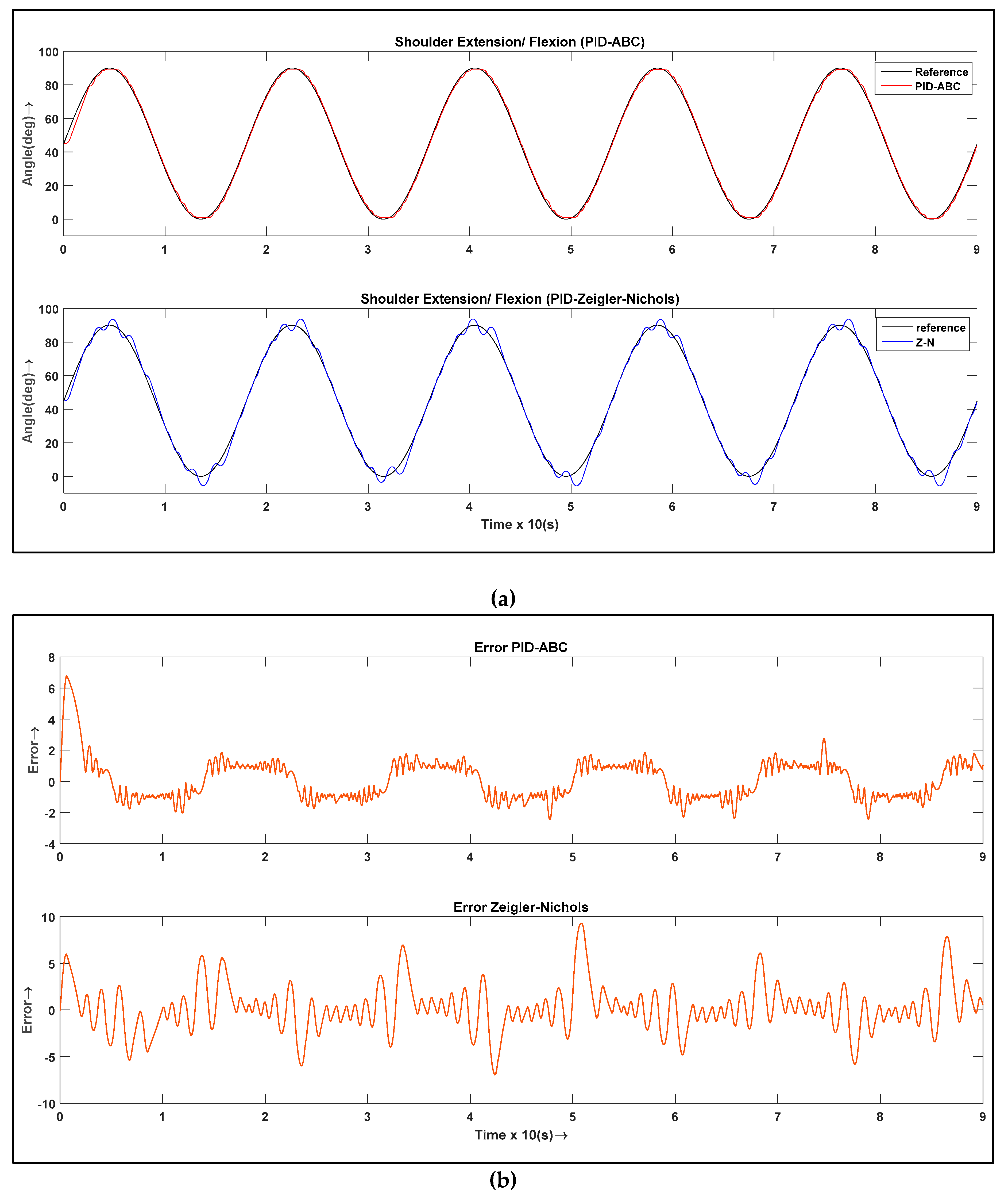
The Zeigler-Nichols is a heuristic algorithm based on increasing proportional gain until it reaches the ultimate gain at which output of a control loop system has consistent oscillations. The parameters $K_u$ and oscillation period $T_u$ are used to parametrize PID gains. Using such a controller produces oscillations which introduce large overshoot, higher rise times and lower settling time in the response.

GA is based on the theory of biological operations and optimizes parameters using mutations and crossover operations [12]. ACO is an evolutionary algorithm inspired by the social behavior of ants searching for food using the shortest path. The success rate of ACO is lower than that of PSO [13]. Fuzzy logic is another technique to optimize the parameters of PID. The rehabilitation robot is controlled by PID and the parameters of PID are optimized using fuzzy logic. Every parameter of the PID controller is characterized by different sets of fuzzy rules, and triangular membership functions are used. Experimental results showed that fuzzy PID offers improved and more effective trajectory tracking performance compared to conventional PID controllers [14,15].

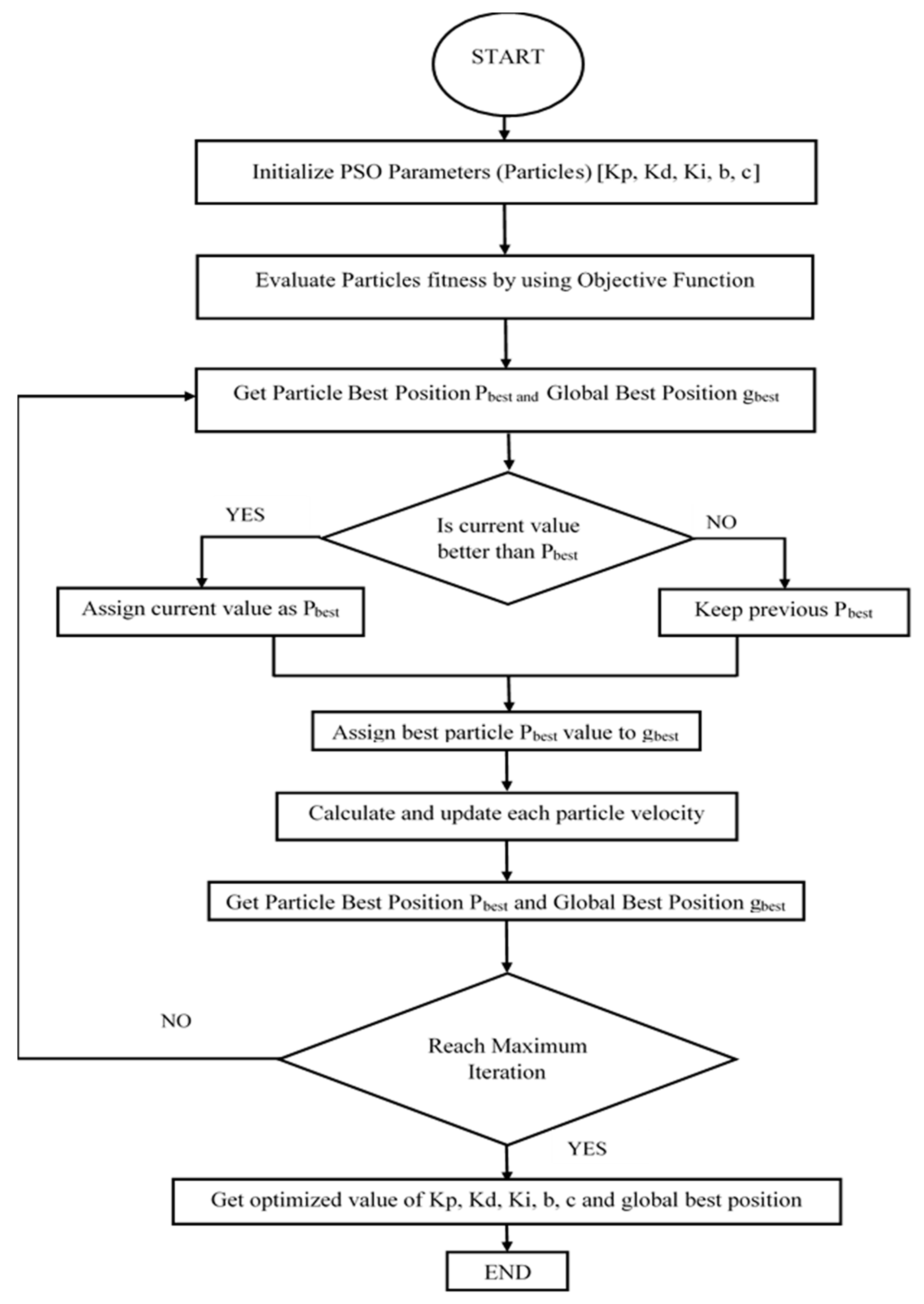
PSO algorithm is an evolutionary computation technique inspired by the social behavior of swarms and fish schools. It was first introduced by Eberhart and Kennedy in 1995. Later Eberhart and Shi introduced inertial weights for PSO to provide the global and local exploration balance. PSO has been found to be robust in optimizing nonlinear problems. The PSO technique evaluates the particle position and velocity, which are updated on every iteration with the aim to reach a global best position of the swarm. Every particle in PSO is treated as a volume-less particle in the search space. PSO requires fewer computational resources than GA, which is prone to premature convergence, while its convergence rate is slower than PSO and ABC [16]. PSO is widely used in many engineering applications because of its advancements. Previously, a PSO based optimized PID controller was used to control a multi fingered robotic hand. Comparison of PSO and conventional PID with fuzzy PID is also presented in the work which shows the better results of PSO-PID [17].

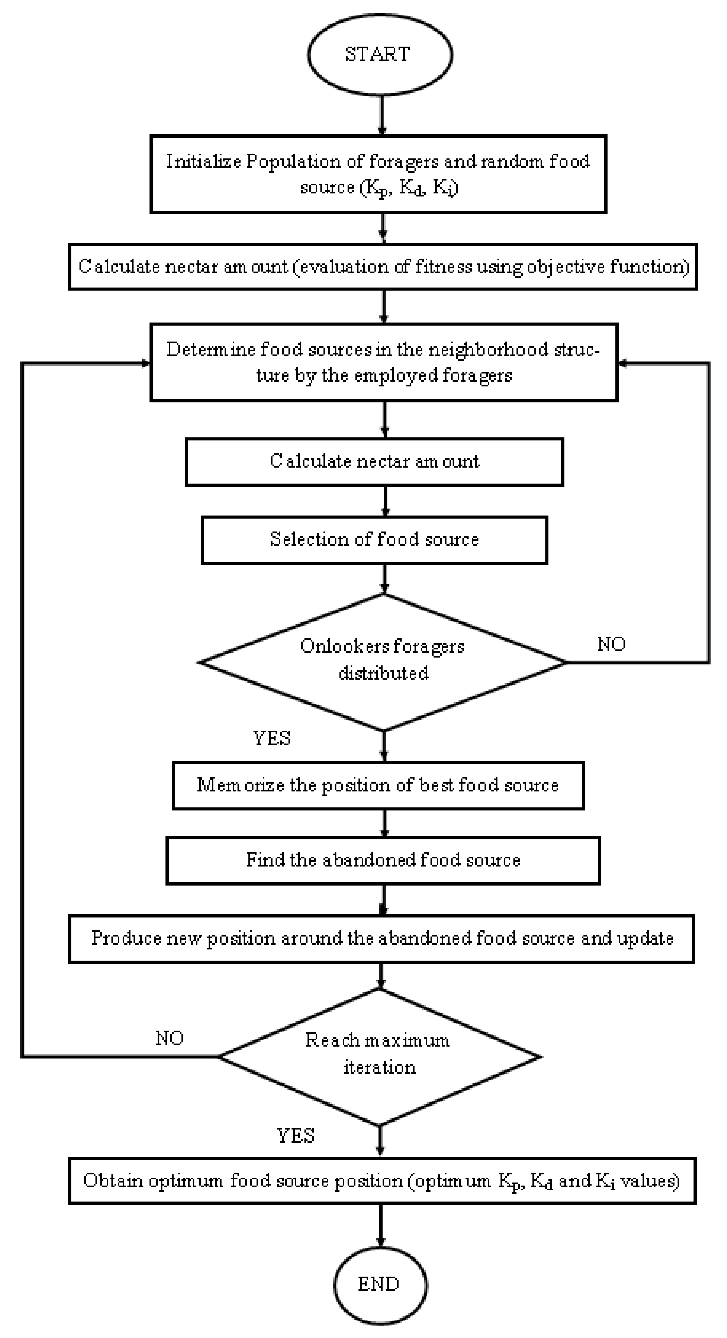
ABC is a heuristic technique which is inspired by the intelligent foraging behavior of honeybees. It was proposed by Karaboga in 2005 [11], and is a simple, robust and population based stochastic optimization algorithm [16,18]. The following three categories of bees make the algorithm unique as compared to other swarm algorithms: employed, onlookers and scout bees [19]. In particular, this meta-heuristic algorithm replicates the foraging behavior of honey bees, where a foraging bee evaluates several characteristics of a food source, such as richness of nectar and the complexity of extracting the energy, and communicates the position of the food source to unemployed bees. The communicated information includes the direction and distance to the food source and its profitability; it is regularly updated so that the best food source can be determined. 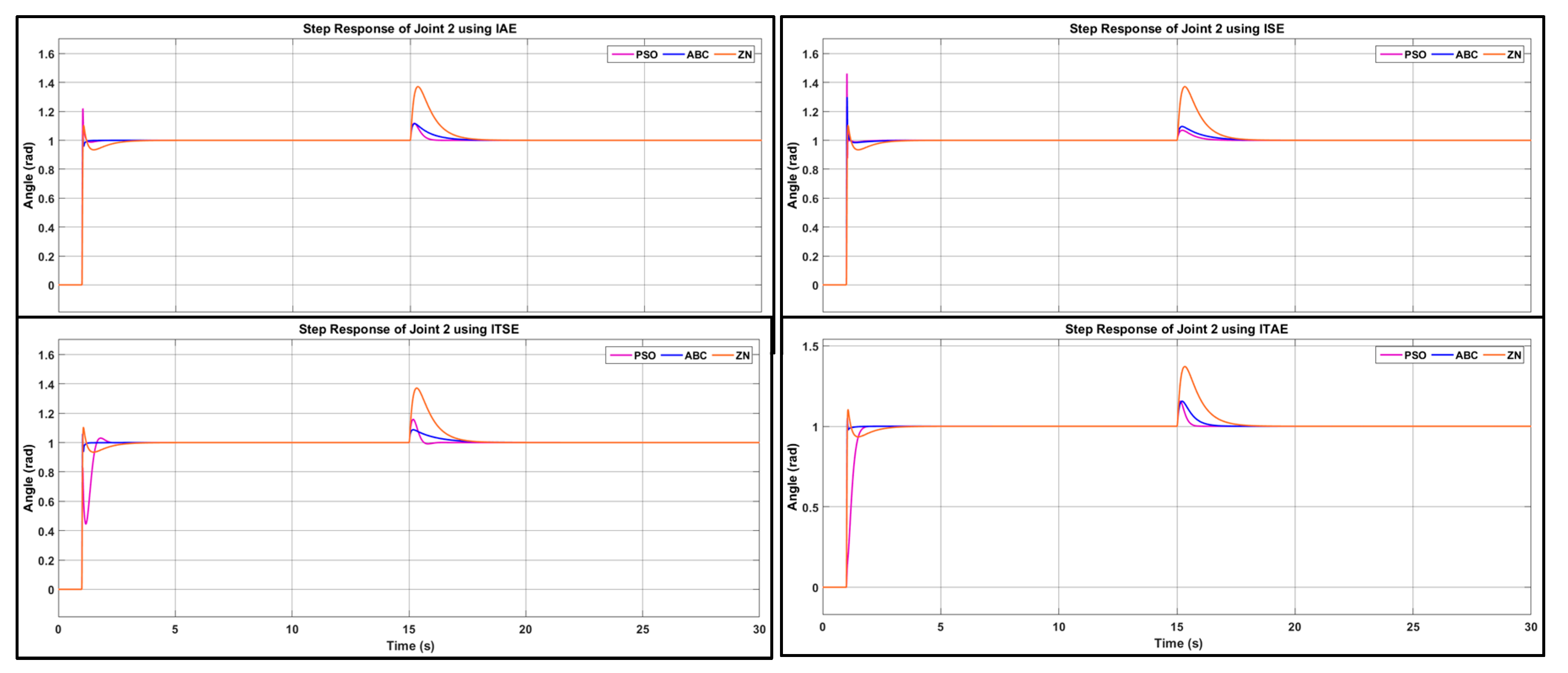In a recent study, a comparison reported that by using integral square error (ISE) as the objective function to optimize PID, better performance was obtained using PSO than ABC [14]. However, in terms of transient time response that overshoots in the response of system, the rise and settling times of ABC is better than PSO. Although the rise time of PSO is faster than ABC, in rehabilitation, high speed is not recommended, so the slow rise times of ABC eventually offer the benefit of safe movement of the robot and avoid abrupt movements. Also, the ABC algorithm outputs high quality solutions in terms of fitness value with fewer function evaluations in comparison to PSO. It was found that ABC is more robust than PSO optimized controller [20].

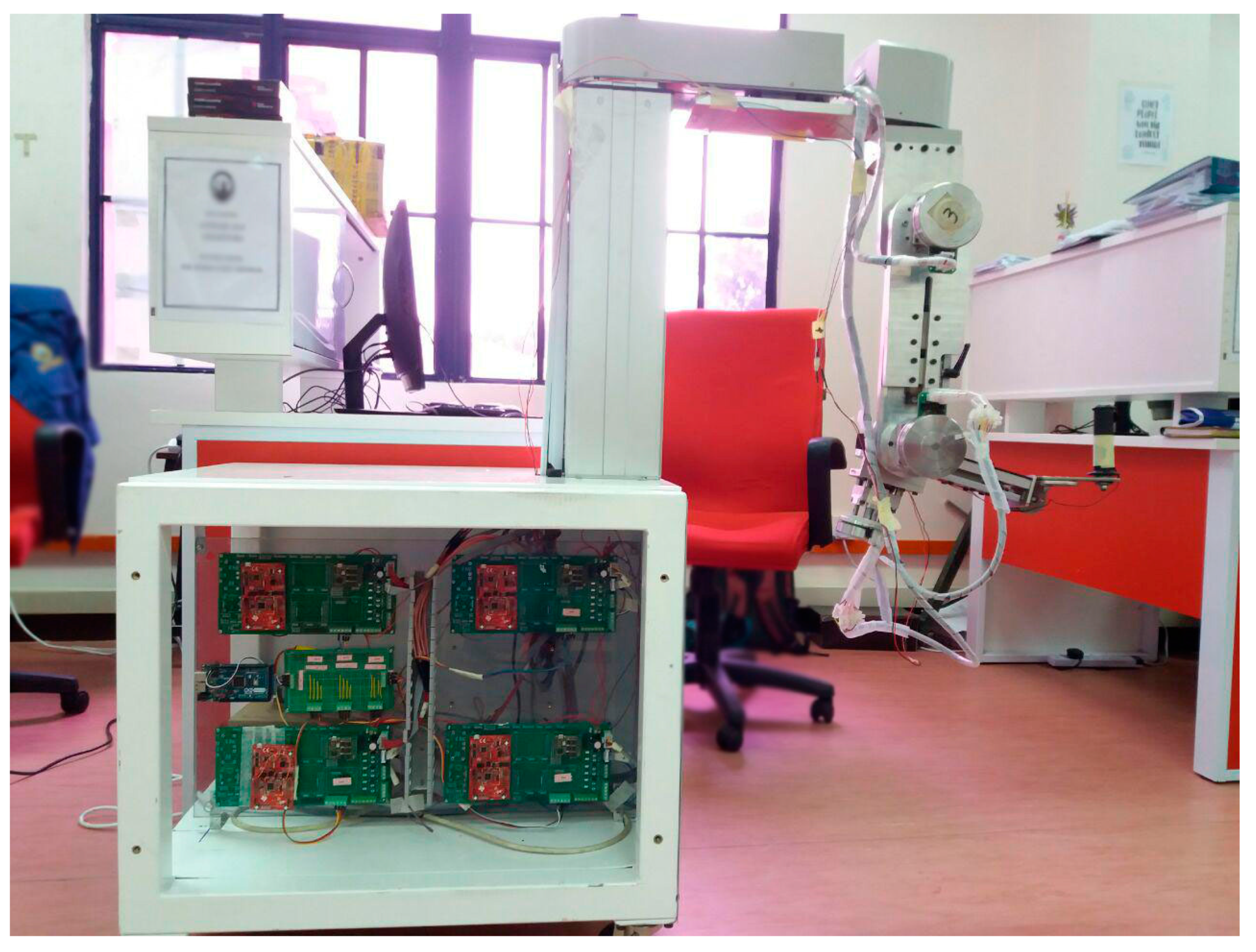
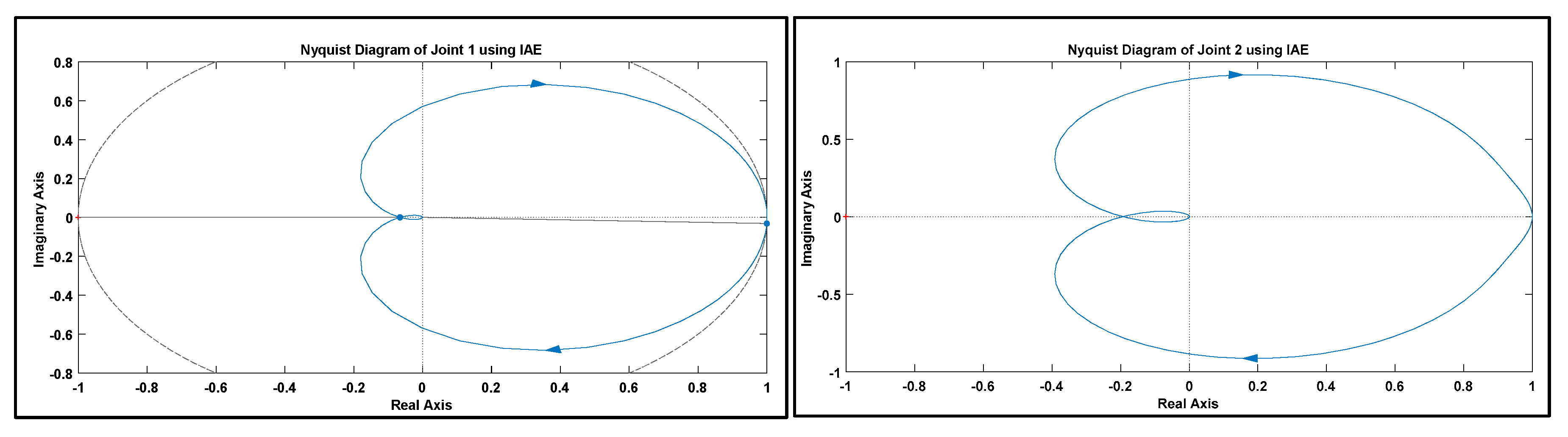
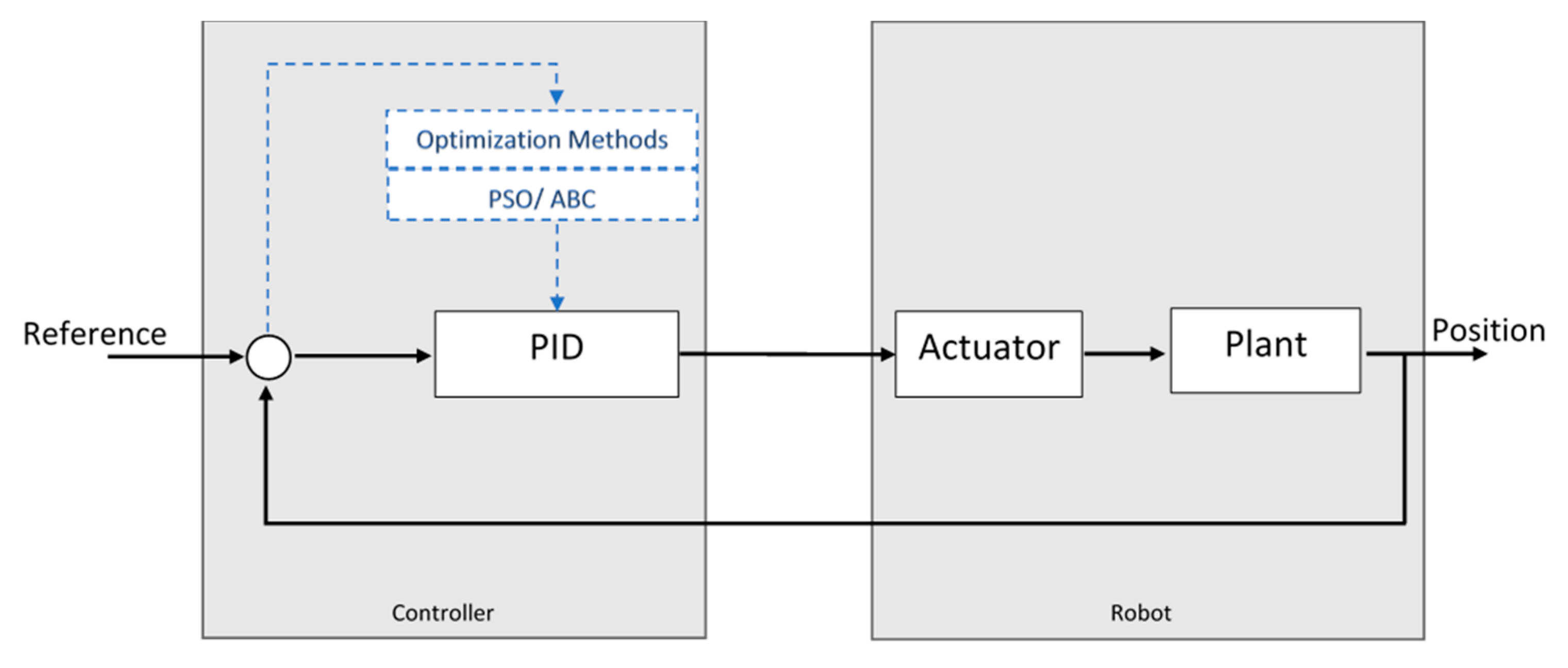
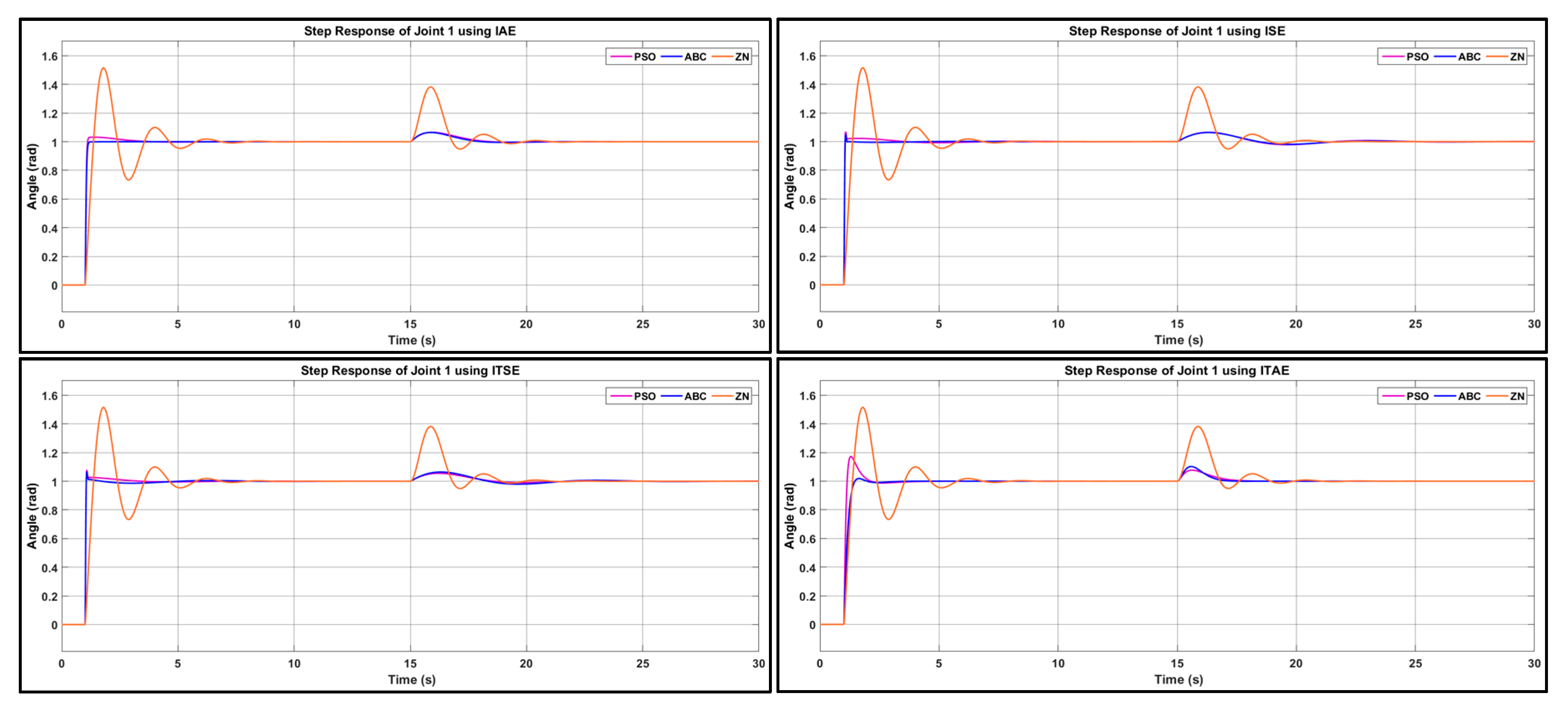
This paper presents a comparative analysis of Zeigler-Nichols, ABC and PSO to determine the tuning parameters of a two-degree-of-freedom (2-DOF) PID controller for robotic arm exoskeleton RAX-1. The objective of applying the mentioned optimization algorithms is to establish the optimal control parameters of the 2-DOF PID by minimizing cost, and to meet the prescribed performance criteria. Four different objective functions, i.e., integral square error (ISE), integral time square error (ITSE), integral absolute error (IAE) and integral time absolute error (ITAE), have been investigated to find the controller with optimal or near optimal load disturbance response subject to robustness and maximum sensitivity constraints. Maximum sensitivity represents the inverse of the minimum distance on the Nyquist plot between critical point and loop transfer function. Such a method for tuning the controller parameters has proven to be effective for robust performance [21]. Furthermore, performance parameters such as overshoot, rise time, settling time and maximum sensitivity are normalized and the least average error (LAE) is evaluated. The optimal solution found for 2-DOF PID for RAX-1 is then implemented with the RAX-1 hardware for trials with three healthy subjects. The rest of the paper is organized as follows. Section 2 explains the controller design, Section 3 presents the simulation results, Section 4 provides the comparative analysis and discussion. Section 5 concludes the paper.

2. Methodology

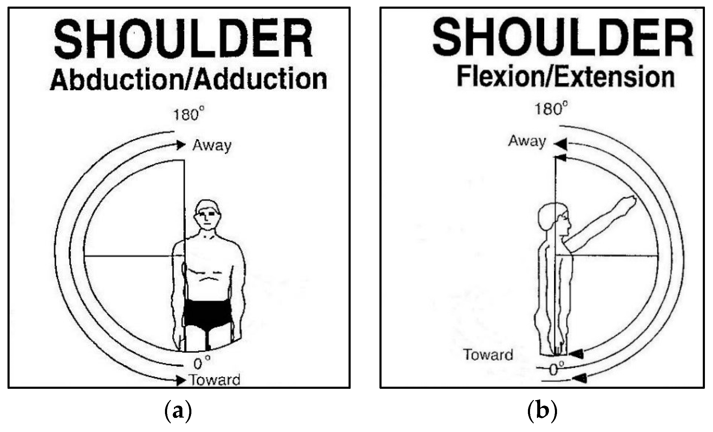
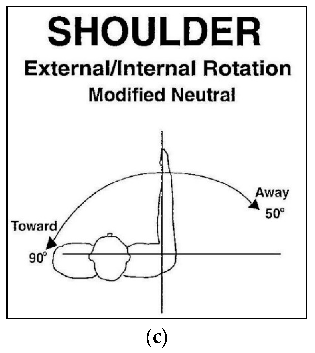
RAX-1 is an exoskeleton device meant to be used for rehabilitation of upper limb extremities. Operating alongside the human arm, exoskeleton devices are required to produce movements similar to those performed by the upper limb. There are nine DOFs in the upper limb, excluding finger joints. This study focuses on the glenohumeral joint in the shoulder, which is a complex ball-and-socket joint that enables the shoulder to perform movements in three DOFs. These movements are commonly referred to as shoulder extension/flexion, abduction/adduction and medial/lateral rotation, also known as internal/external rotation. Figure 1 represents the three movements that can be performed with the shoulder joint. The ranges of motion for the shoulder joint movements performed by a healthy subject are listed in

Table 1. Standard ranges of motion of Upper Limb.

Limb	Therapeutic Exercise	ROM of Limb
Shoulder	Flexion/extension	0°/180°
	External/internal rotation	50°/90°
	Abduction/adduction	0°/180°

[22]. These movement protocols are then implemented on RAX-1.

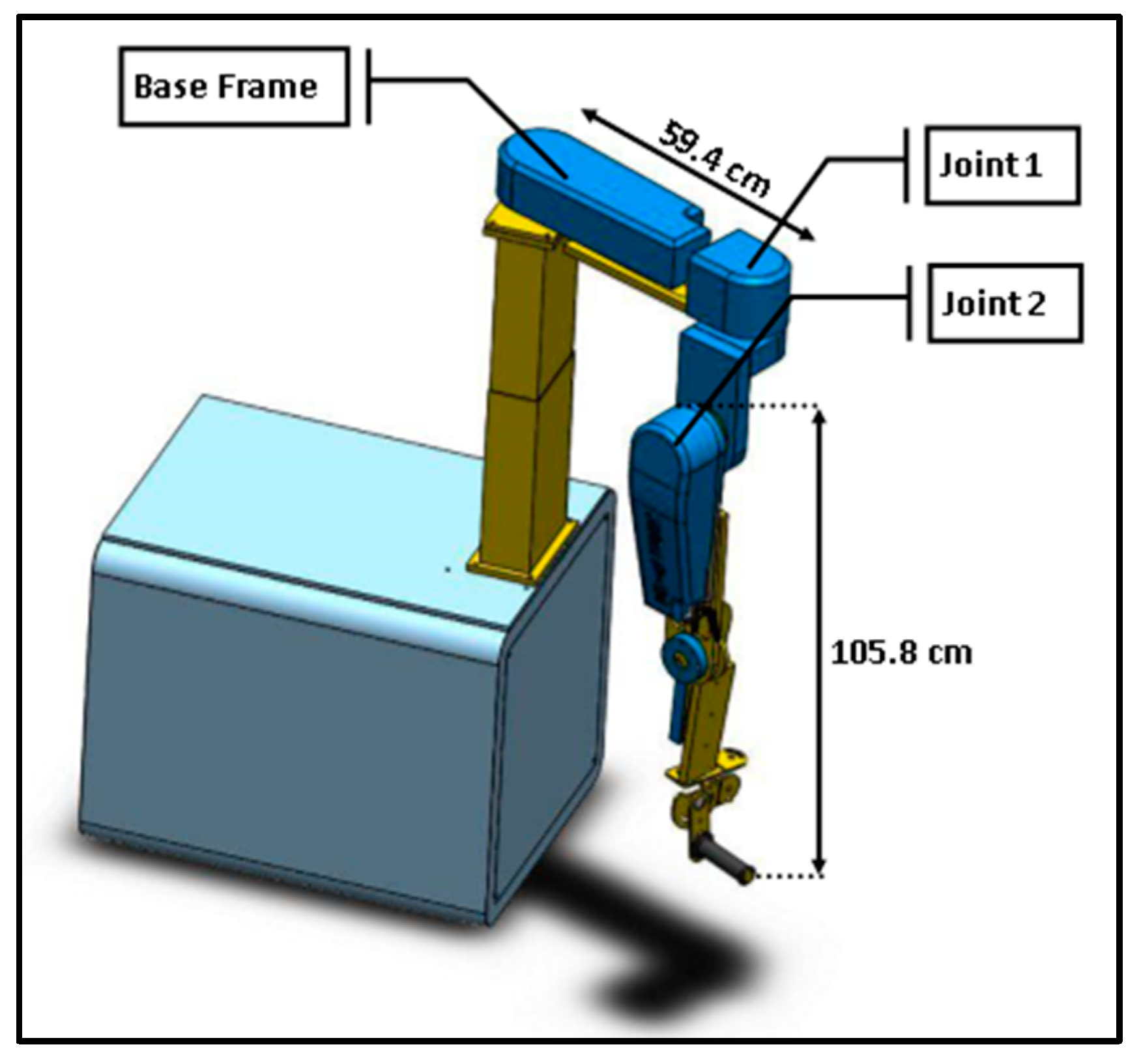
2.1. System Design

The robotic manipulator in the present study comprises two shoulder joints. The DOF of the manipulator can be calculated by the numbers of links and joints. The 3D model of the robot is illustrated in Figure 2.

A robot in the planner configuration is defined with three parameters (x, y, θ). However, robots are three dimensional in real-world applications; hence, there is a need for six parameters (x, y, z, yaw, pitch, roll) to describe the position and orientation of a robot in space.

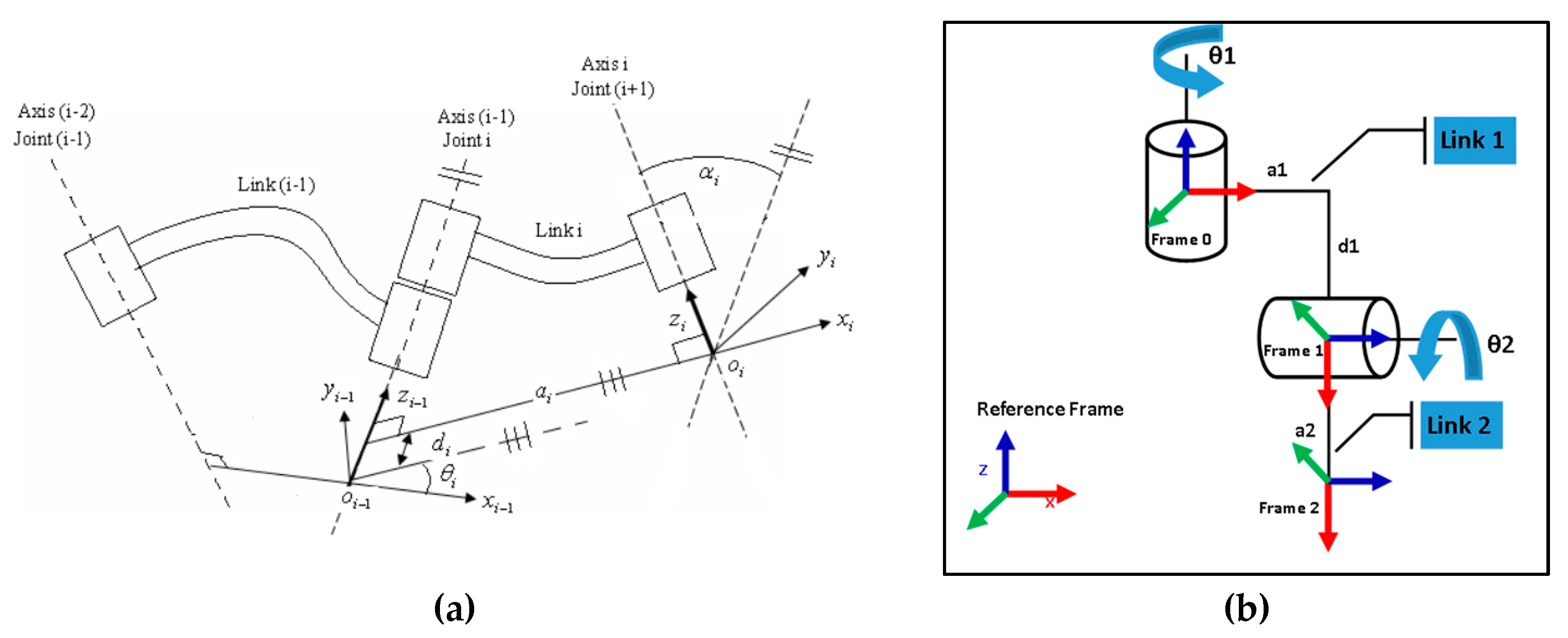
Figure 3 represents the direct kinematics of the robotic arm. Every rigid body in a serial chain has a label: Link 1 is the rigid body attached to the shoulder joint 1, Link 2 is the rigid body attached to Link 1 and so on. A joint is present between each link. Hence, Joint 1 attaches Link 1 to Link 0 and Joint 2 attaches Link 2 to Link 1. Frame of reference is numbered according to the respective links they are attached to, e.g. Frame 1 is attached to Link1. Eventually, the aim is to calculate the position of Frame 2 relative to that of Frame 0.

Figure 3a shows a pair of adjacent links which are link (i − 1), and link (i) with their associated joints, joint (i − 1), and joint (i). A frame (i) is assigned to link (i) as follows.

• The z_{i − 1} lies along the axis of motion of the ith joint.
• The x_i axis is normal to the z_{i − 1} axis and pointing away from it.

The Denavit-Hartenberg (DH) parameters of a rigid link depends on four geometric parameters (a_i, α_i, d_i, θ_i) [23]. The four parameters describe any revolute joint as follows:

• a_i (Link length) is a distance measured along the x_i axis from the point of intersection of x_i axis with z_{i − 1} axis to the origin of frame (i).
• α_i (Link Twist) is the angle between the joint axes z_{i − 1} and z_i axes measured about x_i axis in the right-hand orientation.
• d_i (offset) is the distance measured along z_{i − 1} axis from the origin of frame (i − 1) to the intersection of x_i axis with z_{i − 1} axis.
• θ_i (Joint angle) is the angle between x_{i − 1} and x_i axes measured about the z_{i − 1} axis in the right-hand sense.

The 2-DOF upper limb robotic manipulator can be calculated from Figure 3b. The transformation matrix from Frame 0 to the end-effector can be defined as:

$$T_0^e=\left[\begin{array}{cccc}{c}_{12}& c_1{s}_2& -s_1& a_2{c}_{12}+a_1{c}_1\\ s_1{c}_2& -s_{12}& c_1& a_2{s}_1{c}_2+a_1{s}_1\\ -s_2& -c_2& 0& a_2{s}_2+d_1\\ 0& 0& 0& 1\end{array}\right]$$

where $a_1=59.4$ cm, $a_2=105.8$ cm and $d_1=20$ cm. The transformations can be used to determine kinematic measurements of the joints. For any joint angle, the position of the end effector can be derived from the transformation matrix.

2.2. Dynamic Model

In this study, Euler-Lagrangian approach was applied to calculate the dynamics of the robot manipulator. This approach uses the joint velocities and position to determine the kinetic and potential energies of a system. It generalizes Newtonian mechanics for systems that are subject to a specific class of constraints. These constraints are often expressed in terms of the position or variables describing the system in question.

The Lagrangian equation of motion defined in (1) is written as:

$$\frac{d}{dt}\left(\frac{\partial L}{\partial \dot{q_j}}\right)-\frac{\partial L}{\partial q_j}={\tau }_j$$

(1)

where ${\tau }_j$ denotes the required torque, L = K − P (Kinetic and potential energies) is the Lagrangian and qj is the generalized coordinate of the jth joint of robot.

The inertial matrix $D\left(q\right)$ can be determined as follows:

$$D\left(q\right)=m_1{J}_{vc1}^T{J}_{vc1}+m_2{J}_{vc2}^T{J}_{vc2}+\left[\begin{array}{cc}{I}_1+I_2& 0\\ 0& I_2\end{array}\right],$$

(2)

where $m_1=1.5 \mathrm{kg}$, $m_2=0.5 \mathrm{kg}$. Simplifying (2), one can obtain the following (3).

$$\begin{array}{c}{d}_{11}=m_1{a}_{c1}^2+2m_2{a}_1{a}_{c2}{c}_2-2a_{c2}{d}_1{m}_2{s}_2+a_1^2{m}_2+a_{c2}^2{m}_2+d_1^2{m}_2+I_1+I_2\\ d_{12}=m_2{a}_1{a}_{c2}{c}_2-m_2{d}_1{a}_{c2}{s}_2+m_2{a}_{c2}^2\\ d_{21}=m_2{a}_1{a}_{c2}{c}_2-m_2{d}_1{a}_{c2}{s}_2+m_2{a}_{c2}^2\\ d_{22}=m_2{a}_{c2}^2+I_2\end{array}$$

(3)

The correction term Christoffel symbols ensures that when the derivatives of the vector field lying in a tangent plane of the configuration manifold are computed, they stay in the same tangent space. The Christoffel symbols in (4) are defined as

$$\begin{array}{c}{c}_{111}=\frac{\partial d_{11}}{\partial q_1}=0\\ c_{121}=c_{121}=\frac{1}{2}.\frac{\partial d_{11}}{\partial q_2}=-m_2{a}_1{a}_{c2}{s}_2-m_2{d}_1{a}_{c2}{c}_2=h\\ c_{221}=\frac{\partial d_{12}}{\partial q_2}-\frac{1}{2}.\frac{\partial d_{22}}{\partial q_1}=h\\ c_{112}=\frac{\partial d_{21}}{\partial q_1}-\frac{1}{2}.\frac{\partial d_{11}}{\partial q_2}=-h\\ c_{122}=c_{212}=\frac{1}{2}.\frac{\partial d_{22}}{\partial q_1}=0\\ c_{222}=\frac{1}{2}.\frac{\partial d_{22}}{\partial q_2}=0\end{array}\}$$

(4)

The potential energy of each joint $P_i$, is the product of the mass of that link $m_i$, position vector to the centre of mass $r_{ci}$ and acceleration due to gravity $g$:

$$P_i=m_{i}g{r}_{ci}; i=1,2$$

(5)

The term ${\varphi }_k$ is a function of generalized coordinates that does not depend on their derivatives. It is given by the partial derivative of potential energy of the system with respect to the generalized coordinates as follows:

$${\varphi }_k= \frac{\partial P}{\partial q_k}$$

(6)

Finally, the dynamic equations of the system after substituting various quantities and omitting zero can be expressed as

$$\begin{array}{c}{d}_{11}{\ddot{q}}_1+d_{12}{\ddot{q}}_2+c_{121}{\dot{q}}_1{\dot{q}}_2+c_{211}{\dot{q}}_2{\dot{q}}_1+c_{211}{\dot{q}}_2{}^2+{\varphi }_1={\tau }_1\\ d_{21}{\ddot{q}}_1+d_{22}{\ddot{q}}_2+c_{112}{\dot{q}}_1{}^2+{\varphi }_2={\tau }_2\end{array}\}$$

(7)

which, in general can be written in matrix form as:

$$D\left(q\right)\ddot{q}+C\left(q,\dot{q}\right)\dot{q}+g\left(q\right)=\tau$$

(8)

Here,$D\left(q\right)$ denotes the inertia matrix of the system and $C\left(q,\dot{q}\right)$ gives the Christoffel symbols and $g\left(q\right)$ is actually ${\varphi }_k$ which is determined by taking partial derivative of potential energy with generalized coordinates. $\tau$ is a 2 × 1 matrix representing the generalized active forces.

2.3. Linearized Model

The linearized state space model for robot exoskeleton (RAX-1) is expressed as follows.

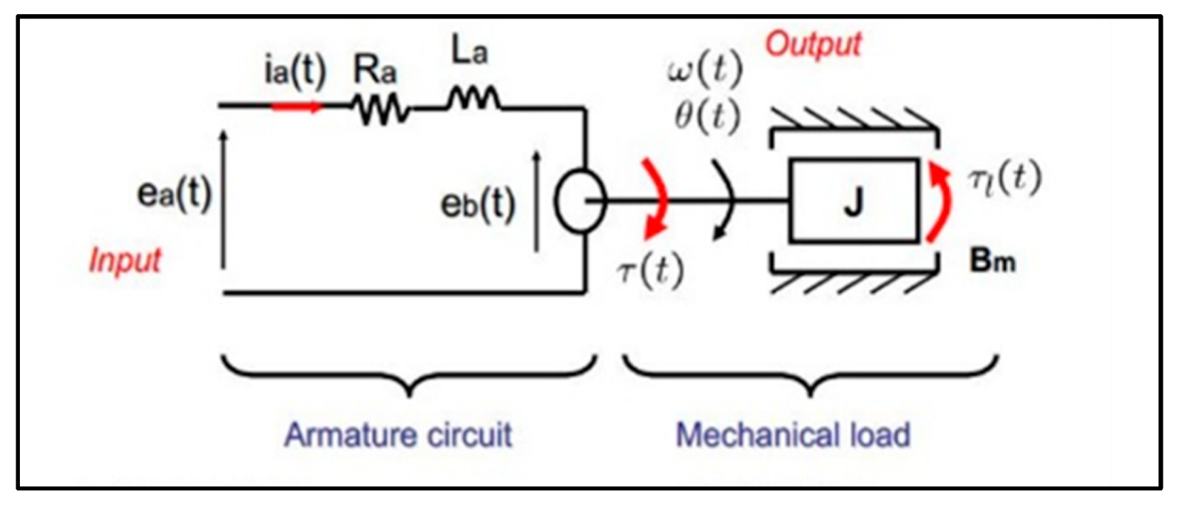
$$\begin{array}{c}A=\left[\begin{array}{cccc}0& -5.5510e-13& 0& 0\\ 1& 0& 0& 0\\ 0& 0& 0& -25.8600\\ 0& 0& 1& 0\end{array}\right],B=\left[\begin{array}{cc}1& 0\\ 0& 0\\ 0& 1\\ 0& 0\end{array}\right]\\ C=\left[\begin{array}{cccc}0& 31.66& 0& 0\\ 0& 0& 0& 6.3760\end{array}\right],D=\left[\begin{array}{cc}0& 0\\ 0& 0\end{array}\right]\end{array}$$

(9)

2.4. Motor Model

The robot manipulator requires actuators to provide the desired amount of torque at the joints. The actuators convert electrical energy into rotational mechanical energy. DC motors are widely used in robotics as actuators due to their high torque, speed controllability and portability [24]. The internal model of DC motor is illustrated in Figure 4 and can be expressed as follows.

$$\frac{\theta \left(\mathrm{s}\right)}{{\mathrm{E}}_{\mathrm{a}}\left(\mathrm{s}\right)}=\frac{K_{\tau }}{\left(L_{a}s+R_a\right)\left(Js+B_m\right)+K_b{K}_{\tau }}\approx \frac{K_{\tau }}{R_a\left(Js+B_m\right)+K_b{K}_{\tau }}$$

(10)

Here,’$J$’ is the motor inertia, ‘$B_m$’ motor damper, ‘$K_{\tau }$’ is the motor constant, ‘$K_b$’ is the proportionality constant between angular velocity of the motor and back emf, whereas ‘$L_a$’ and ‘$R_a$’ inductance and resistance of the armature. If $L_a\ll R_a$ then, an approximated transfer function of motor is obtained by setting $L_a=0$. This converts motor model from a second order system to 1st order system. DC motors with harmonic gears are used in this system.

Table 2. Motor Parameters.

Parameters	Joint 1	Joint 2
Kτ (mN-m/A)	70.5	70.5
La (mH)	0.264	0.264
Ra (Ohm)	0.343	0.343
Kb (V-s/rad)	0.023	0.023
J (g·cm²)	306 × 10−6	306 × 10−6
Bm (N.sec/m)	0.03	0.03
Gear Ratio (Nm/Nl)	1/160	1/150

lists the motor parameters.

3. The Exoskeleton Platform

In this section, the hardware design for the upper limb extremity rehabilitation is described. The platform consists of the design and manufacturing of the mechanical structure, actuators and sensors with hardware implementation of the control algorithm.

3.1. Mechanical Structure

The 2-DOF mechanical platform is built using aluminum grade 6061 alloy and weighs approximately 15 kg. The structure is specifically designed to focus on specific exercises for rehabilitation of the shoulder joint (Figure 5).

The upper extremity exoskeleton device consists mainly of a support frame, height adjustment mechanism and shoulder actuation mechanism. The support frame is attached to wheels enabling the platform to be remote. The manually controlled height regulation mechanism is attached to the support frame. The actuation mechanism is attached to the height regulation mechanism; it adjusts the mechanical frame fixed to human arm to match requirements to the subject height. The human arm is fixed to the exoskeleton with soft wraps both on the forearm and bicep. Other relevant adjustments are made during gait training. Joints at the wrist and elbow are passive and their orientations are fixed.

3.2. Actuators and Sensors

The two-revolute joint system is equipped with the MAXON EC-90 motor (Maxon Motor, Sachseln, Switzerland) attached to the gear. A brushless flat motor has the maximum angular velocity of 2590 rpm and power rating of 90W which can generate maximum torque of 444 mNm. It is equipped with three Hall effect sensors to measure current and velocity and an internal encoder generating 2040 pulses per rotation. The reducers (harmonic drives) combined with flat motor have speed ratio of 160:1 for the first shoulder joint responsible for the internal/ external movement, while the ratio is 150:1 for the other joint responsible for the extension/ flexion movement. The detailed specification of other motor parameters and gear ratio is provided in Table 2. A force sensor is attached to the wrist handle of the robot, from which external disturbance exerted by the subject is measured while the exoskeleton is working in passive mode. The electrical setup of the system involves an ESCON 50/5 module which acts like a closed-loop speed or current controller for the motor.

3.3. Control Implementation

In the control system, a host computer is used as a graphical user interface. The software is written in visual C#; it allows the user to select one of the possible working modes of the exoskeleton (passive, active or semi-active). The software enables uploading and downloading subject’s history over a cloud specifically designed for this device. The user can also define the range of motion at which the exoskeleton should work for several repetitions.

A master/slave network is designed to interconnect the user with the system, where each joint in the system is a slave. CC3200 from Texas Instrument is used as a peripheral device that controls the angular movement. The master is instructed by the user to select an exercise and the number repetitions, as well as set an angular movement via an interface. This information is then communicated to the slaves for further implementation of the task [25] as depicted in Figure 6a,b. The overall system block diagram is illustrated in Figure 6c.

Figure 7 represents the controller card used for RAX-1; it consists of master-slave network and drivers used for motors.

4. The Control Algorithm

4.1. Proportional Integrator Derivative (PID) Controller

One of the most widely used controllers is the PID controller, which has a very simple structure and is robust in under wide range of operating conditions. The PID error signal, which is the difference between setpoint and measured variable, is calculated and fed back into the system continuously to change the proportional, integral and derivative gains accordingly [26].

PID is one of the most used control algorithms in industrial control systems. The response of a system is categorized by the rise time, overshoot, settling time and steady state error. In this study, a 2-DOF PID controller is used, and is represented mathematically according to Equation (11). The controller is capable of rejecting disturbances without significant increase of overshoot in setpoint tracking. It includes setpoint weighting on the proportional and derivative terms. A typical 2-DOF PID is composed of feed-forward and feedback compensators. The feed-forward compensator consists of a PD component while the feedback compensator includes PID component as shown in Figure 8.

$$u=K_p\left(b.r-y\right)+K_i\left(r-y\right)s^{-1}+K_d\frac{N}{1+N{s}^{-1}}\left(c.r-y\right)$$

(11)

where $u$ denotes the input given to the plant or system, while $K_p$, $K_d$, $K_i$, denotes the proportional, derivative and integral gains. In this study, 2-DOF PID in MATLAB is used, which has three more parameters to tune; b, c and N, where; $b$ and $c$ denote the setpoint weights, while $N$ denotes a filter coefficient.

4.2. Particle Swam Optimization (PSO)

PSO is an optimization technique inspired by the social behavior found in nature, such as flocking of birds and fish schooling. In the PSO search space, each solution acts like a flying bird in the search of food, known as a particle. PSO works based on the social behavior of particles in a swarm. This algorithm locates and finds the global best solution by adjusting an objective function. At the end of the process, best solution based on objective function is found for 2-dof pid controller parameters.

First, PSO chooses random solutions to initialize the population. Then, it updates its performance to obtain optimum value. Every particle is characterized by its position and velocity in the swarm. The velocity of a moving particle depends upon the change in position or direction [27]. Each particle updates its new position based on two components, p_best and g_best, where p_best is the best position attained by a particle, while g_best is the global best position of the entire swarm. The velocity and position of the particle can be expressed according to Equations (10) and (11), respectively.

$$v_{ij}\left(t+1\right)=w{v}_{ij}\left(t\right)+r_1{c}_1\left(p_{ij}\left(t\right)-x_{ij}\left(t\right)\right)+r_2{c}_2\left(g_j\left(t\right)-x_{ij}\left(t\right)\right)$$

(12)

$$x_{ij}\left(t+1\right)=x_{ij}\left(t\right)+v_{ij}\left(t+1\right)$$

(13)

where; $v_{ij}\left(t\right)$ denotes the particle velocity, $x_{ij}\left(t\right)$ denotes the particle position, $v_{ij}\left(t+1\right)$ denotes the particle updated velocity, $x_{ij}\left(t+1\right)$ denotes the particle updated position; $p_{ij}\left(t\right)$ denotes the particle best position; $g_j\left(t\right)$ denotes the global best position of the swarm; $w ,\left(w=w_{max}-w_{min}\right)$ denotes the inertia term; $r_1$ and $r_2$ are two uniformly distributed random numbers ranging from 0 to 1 and $c_1$ and $c_2$ are the acceleration coefficients. The important steps of the PSO are summarized in Figure 9.

According to the PSO algorithm, the swarm size, position, velocity and the constants $w$, $c_1$ and $c_2$ are initialized first. Then, the fitness value of each particle is calculated, $P_{best}$ and $g_{best}$ are defined and the position and velocity of each particle are updated. The algorithm stops when the stopping criterion is met. The optimal solution is chosen according to the latest $g_{best}$. The PSO parameters and their values used in our study are provided in

Table 3. PSO Parameters.

Parameter	Value
Number of particles	20
Number of iterations	150
$w_{min}$	0.4
$w_{max}$	0.9
$c_1$	2
$c_2$	2

.

4.3. Artificial Bee Colony (ABC)

ABC is an optimization technique based on the smart behavior of honey bees [16], which are famous for their intelligence and ability to perform complex tasks such as collecting nectar and building nests with a high degree precision [28]. Information about the quality of a food source is communicated within the colony by a particular dance language. The precision of the foraging range of honeybees allows an efficient exploitation of food sources and concentration of foraging on the best patches. There are two main concepts that describe swarm intelligence, namely self-organization and labor division [29]. The self-organizing behavior represents the complex collective behavior that rises from the local interaction between the agents showing a simple self-directed behavior. The mechanism of labor division assigns specific tasks to the agents performing simultaneous activities, which results in a more efficient and time-saving performance.

There are three categories of artificial bees in ABC algorithm: employed, scout and onlooker bees. The employed bees go to the food source that has already been visited by them, while unemployed bees look for further sources of food. The number of employed bees is equal to that of food sources. Searching for new sources is performed by the scout bees, whereas the onlooker bees wait for the information about the discovered food sources provided by employed bees via their waggle dance. If the position of a food source does not improve within a number of attempts known as limits, then the employed bees become scout bees. In this manner, the exploitation process is performed by employed and onlooker bees, whereas the scout bees explore the existing solutions. The details of different ABC phases are described in the following subsections.

a. Initialization Phase

Random initialization of the locations of food sources is performed according to the following equation:

$$x_{ij}=x_j^{max}+rand\left(0,1\right)\left(x_j^{max}-x_j^{min}\right);i=1,\dots ,SN, j=1,\dots ,D$$

(14)

where SN is the number of food sources taken as half of the bee colony, D is the dimension of the problem, $x_{ij}$ denotes the i^th employed bee on j^th dimension, wjile $x_j^{max}$ and $x_j^{min}$ denotes its upper and lower bounds.

b. Employed Bee Phase

Every other employed bee is allocated with the food source for further exploitation. Equation (11) represents the process of generating a food source.

$$v_{ij}=x_{ij}+\varphi \left(x_{ij}-x_{kj}\right)$$

(15)

where $\varphi =a\times rand\left(0,1\right)$ is a random variable denoting the acceleration coefficients ranging in the interval [−1,1] and $v_{ij}$ is the new solution or a food source. The fitness $fi{t}_i$ of the new food source is calculated according to the following equation:

$$fi{t}_i=\{\begin{array}{c}\frac{1}{1+f_i}, f_i\ge 0\\ 1+abs\left(f_i\right), f_i<0\end{array}$$

(16)

where, $f_i$ is the objective function of each food source. A selection is made between the original and new food sources to choose the better one by keeping the fitness value in accordance.

c. Probabilistic Selection Phase

An onlooker bee selects a food source with a certain probability calculates as

$$p_i=\frac{fi{t}_i}{{{\displaystyle \sum }}_{j=1}^{N}fi{t}_j}$$

(17)

where $p_i$ denotes the probability of selecting the ith solution.

d. Onlooker Bee Phase

The employed bees share the information about food sources with the onlooker bees, who select a food source to exploit better solutions according to its selection probability. The fitness values of each exploited food sources is calculated. A greedy selection between original and new food sources is made similar to the employed bees phase.

e. Scout Bee Phase

If a food source does not yield better results within the limits $L$, where $L=0.6\times \left(Number of optimization parameters\right)\times \left(colony size\right),$ then this food source is abandoned and the bee associated with it becomes a scout bee. In this case, a new source of food is randomly generated according to Equation (15). All phases will continue until the termination criterion is met. The output is the best food source solution. Figure 10 shows the flowchart of the ABC algorithm which depicts the process of 2-dof pid controller optimization.

According to the ABC algorithm, the colony size, position and the constants $L$ and $a$ are initialized first. Then, the fitness value is calculated, and the best food source is defined. The algorithm stops when the stopping criterion is met. The optimal solution is chosen according to the latest $g_{best}$. The ABC parameters and their values used in our study are provided in

Table 4. ABC Parameters.

Parameter	Value
Colony Size	20
Number of iterations	150
$L$ (Abandonment Limit)	72
$a$ (Acceleration coefficient)	1

.

5. Results and Discussions

Based on the simulation, the system is divided into two linearized sub systems representing Joint 1 and Joint 2 [30]. Independent controls for both joints with saturation limits are implemented. A step input is given to the model of the robot and the response is observed. A schematic of the proposed controller’s tuning method based on PSO and ABC is shown in Figure 11.

For this research, a comparative study was carried out with four different cost functions to gauge the appropriate objective function for this study. A well-chosen objective function leads to better performance of the system and meets control design expectations. These objective functions include the integral squared error (ISE), integral time squared error (ITSE), integral absolute error (IAE) and integral time absolute error (ITAE), and are defined as follows:

$$ISE= {\displaystyle \int }{e}^{2}dt$$

(18)

$$IAE= {\displaystyle \int }\left|e\right|dt$$

(19)

$$ITSE= {\displaystyle \int }t.e^{2}dt$$

(20)

$$ITAE= {\displaystyle \int }t.\left|e\right|dt$$

(21)

5.1. Robustness Consideration

Focus on the tuning procedure requires some robustness considerations in the design. This is achieved by using the maximum sensitivity function as a measure of robustness and is given by

$$M_s=\underset{\omega }{\max }\left|S\left(j\omega \right)\right|=\underset{\omega }{\max }\frac{1}{\left|1- C_y\left(j\omega \right)P\left(j\omega \right)\right|}$$

(22)

where $\left|S\left(j\omega \right)\right|\le M_s$. The sensitivity function shows the effect of feedback on the output. Disturbances are attenuated if $\left|S\left(j\omega \right)\right|<1$ and are amplified if $\left|S\left(j\omega \right)\right|>1$. The robustness of the closed loop increases with the decrease in $M_s$. The values for $M_s$ ranging from 1.2 to 2.0 provides reasonable robustness [27].

5.2. Simulation Setup

Before implementing ABC-PID [11] on hardware, simulations are carried out to validate and verify the control algorithm. In this section, a comparative analysis of the PID controller optimized with ABC, PSO, and conventional tuning method based on Zeigler-Nichols is presented. The parametric bounds are provided in

Table 5. Parametric Constraints used for PSO and ABC.

Parameters	Joint 1	Joint 2
$K_p$	0.01 < $K_p$ < 10	0.01 < $K_p$ < 20
$K_i$	0.01 < $K_i$ < 10	0.01 < $K_i$ < 20
$K_d$	0.01 < $K_d$ < 10	0.01 < $K_d$ < 20
$b$	0.01 < $b$ < 1	0.01 < $b$ < 1
$c$	0.01 < $c$ < 1	0.01 < $c$ < 1
$N$	100	200

. The Zeigler-Nichols PID parameters and PID parameters tuned using ABC and PSO used for simulation are provided in

Table 6. Optimized PID Parameters for Joint 1.

Controller	Objective Function	${\mathit{K}}_{\mathit{p}}$	${\mathit{K}}_{\mathit{i}}$	${\mathit{K}}_{\mathit{d}}$	$\mathit{b}$	c
ABC-PID	ISE	7.271	9.7748	10	0.9533	0.9826
	IAE	10	9.9485	5.8094	0.9521	0.9198
	ITSE	7.003	9.9345	10	0.9401	0.9993
	ITAE	7.9219	10	2.339	0.8137	0.6124
PSO-PID	ISE	6.8358	10	10	1	1
	IAE	9.9531	8.8488	6.0963	1	0.9535
	ITSE	10	10	9.9951	1	1
	ITAE	10	10	3.3444	1	1
ZN-PID	-	2.7	2.5714	0.7087	1	1

and

Table 7. Optimized PID Parameters for Joint 2.

Controller	Objective Function	${\mathit{K}}_{\mathit{p}}$	${\mathit{K}}_{\mathit{i}}$	${\mathit{K}}_{\mathit{d}}$	$\mathit{b}$	c
ABC-PID	ISE	8.7359	10	0.7251	1	0.9717
	IAE	7.229	10	0.5594	0.9999	0.7415
	ITSE	10	10	0.6289	1	0.6926
	ITAE	4.8276	10	0.5214	1	0.8247
PSO-PID	ISE	11.011	20	1.1377	1	1
	IAE	6.1177	20	0.5864	1	0.9625
	ITSE	4.0505	20	0.4883	0.1	0.8429
	ITAE	4.7981	20	0.3883	0.1	0.1
ZN-PID	-	1.92	2.7429	0.3360	1	1

. The simulations presented here are for internal/external rotation, extension/flexion and abduction/adduction of the shoulder joint.

To evaluate the fitness of the objective function, normalization of the objective function is carried out, which scales objective function within a specified range. The following normalization function is used [31].

$$fi{t}_i^{\text{'}}=\frac{fi{t}_i-min\left(fi{t}_{overall}\right)\times \delta }{\max \left(fi{t}_{overall}\right)-min\left(fi{t}_{overall}\right)\times \delta }$$

(23)

where $fi{t}_i$ represents the objective to be normalized and $fi{t}_{overall}$ represents the overall fitness. $\delta$ is kept 0.99 to avoid any zeros during normalization. Furthermore, normalized average has been evaluated to determine the significance of the objective function.

Table 8. Performance Controller Parameters for all Objective Function.

Controller	Integral Absolute Error
		Joint 1						Joint 2
	Best Cost	O.S (%)	R.T (s)	S.T (s)	Disturbance O.S (%)	Ms	Normalized Average	Best Cost	O.S (%)	R.T (s)	S.T (s)	Disturbance O.S (%)	Ms	Normalized Average
PSO-PID	0.219	3.1780	0.0641	0.3	6.6	1.24	0.2326	0.0809	22.0742	0.0159	0.1452	11.5	1.62	0.2425
ABC-PID	0.16375	0	0.0750	0.15	6.5	1.23	0.1643	0.1304	4.4458	0.0211	0.1123	11.5	1.62	0.1541
	Integral Squared Error
PSO- PID	0.0292	6.8484	0.0349	0.9244	6.5	1.37	0.4346	0.0192	46.2938	0.0093	0.1243	6.9	2.0	0.3583
ABC-PID	0.0283	4.9856	0.0360	0.1058	6.4	1.37	0.2476	0.0224	29.9438	0.0131	0.1115	9.6	1.80	0.1983
	Integral Time Squared Error
PSO- PID	0.1065	7.7363	0.0345	0.254	5.5	1.38	0.3771	0.2021	3.0304	0.5020	0.9666	15.4	1.50	0.3637
ABC-PID	0.1457	6.5768	0.0350	0.1217	6.4	1.37	0.2762	0.0936	5.9488	0.0192	0.1082	8.7	1.80	0.2863
	Integral Time Absolute Error
PSO- PID	1.8319	17.2245	0.0958	0.9244	7.7	1.15	0.6496	1.0296	0	0.4208	0.6515	15.1	1.43	0.5296
ABC-PID	1.7792	1.8361	0.2748	0.4130	10.2	1.11	0.5541	1.5827	5.1007	0.0216	0.0954	15.6	1.53	0.3708
	-
ZN-PID	-	51.4168	0.2819	4.5369	51.1	1.91	-	-	10.2841	0.0284	1.4003	37.1	1.3168	-

shows that IAE and ITAE used as objective functions produce minimal overshoots and suitable rise and settling times for both PSO-PID and ABC-PID. When using ISE and ITSE, the rise time is small, while larger overshoots are detected. However, it is obvious that the performance parameters of ABC-PID for Joints 1 and 2 are much better in terms of the six performance parameters mentioned above compared to that of PSO-PID or Zeigler-Nichols.

The results plotted in Figure 12 show the response for Joint 1 for PID controller tuned using the Zeigler-Nichols and optimal parameters found with PSO and ABC for all four-objective functions. The figure shows that the ZN response is quicker with a higher rise time, higher settling time and larger overshoot. The results also show a very low percentage of overshoot in the response with a very low steady state error for all four objective functions. However, the optimal response of the system is found while using IAE as objective function.

Figure 13 shows the step response for Joint 2. It is evident from the figure that PID tuned Zeigler-Nichols produces large overshoot than the PID optimized with ABC or PSO. However, the overshoot of ABC is 4.4% which is smaller as compared to 22% overshoot of PSO when using IAE. It was found that PID-ABC has the minimum average of the normalized objective function for Joint 1 and Joint 2. Hence, the ABC-optimized PID controller is found to be robust and stable for practical implementation on a robotic arm manipulator. The performance and robustness obtained by calculating the system percent overshoot, rise time, settling time, cost and sensitivity is presented in Table 8.

Furthermore, an investigation on closed-loop stability analysis is performed by Nyquist plot of the controllers tuned with ABC using IAE for the given systems. The plot for Joint 1 and Joint 2 are shown in Figure 14. It indicates that the both systems are asymptotically stable as no poles lie in the right half of the plane.

5.3. Experimental Evaluation for RAX-1

A preliminary experiment was conducted to test the efficacy and performance of the exoskeleton controlled using the optimized PID controller. Three healthy male subjects participated in the experiment and their properties are listed in

Table 9. Subject properties.

Parameters	Subject 1	Subject 2	Subject 3
age	32	31	28
body mass (kg)	74	70	64
Height (foot)	5.74	5.91	5.68

. Subjects were bound with soft wraps and their preliminary tests were performed before and after the exercise. The tests included measuring the body temperature, heart rate and oxygen levels. The evaluation procedure was approved by the Ethics committee of the University of Kuala Lumpur (UniKL), Kuala Lumpur, Malaysia. All subjects were volunteers who signed consent forms before the experiment. The procedure was completed in the presence of physiotherapists from the Royal College of Medicine Perak, Malaysia. The mechanical structure used for this experiment was RAX-1 illustrated in Figure 5.

In this experiment, the upper extremity exoskeleton, which is a robot in charge of the rehabilitation protocol, provides passive assistance for the subjects. The two actuators follow the specific trajectories of a pre-defined range of motions. The followed trajectory and joint angles can be measured from the encoders. Figure 15 shows a subject performing the shoulder exercises with the assistance of exoskeleton device. The angular rotation of the joint can be set via the interface, and its current position can be observed on the screen.

A ramp/ sinusoidal repetitive input is provided to the shoulder joint to perform three different exercises, namely shoulder extension/flexion, internal/external rotation and abduction/adduction (Table 1).

For this experiment, a combined shoulder external/internal rotation was performed by the first subject; the upper bound movement during external rotation was limited to 90° and that during internal rotation was limited to 0°. Figure 16a illustrates the motion tracking of the robotic arm where a minute overshoot was observed in reaching the target reference. The graph also shows the error representation between the reference and actual response and speed of the motor in terms of rpm. During the experiment, each subject went through the same gait pattern, i.e. the movement was set to a frequency of 0.25 Hz for internal/external rotation.

Figure 16b shows the current required by the motor to move the shoulder to a desired angle. It also represents the amount of external force exerted by the patient on the system. The external force acts as an external disturbance to the system and its effect can be seen in the Figure 16b. As the external force to resist the movement increases, the motor current drastically increases to overcome the effect of disturbance. The maximum current drawn by the motor is 5.27 A when the maximum external resisting force of 68 N is applied to the joint.

The second exercise, namely shoulder abduction/adduction, was performed by the second subject; the bounds are set from 0° to 90°. Figure 17a represents the response of the system during shoulder abduction and adduction. It also represents the difference between the reference signal and response, which demonstrates a minute overshoot in the response. The gait pattern for this exercise is similar to that for the previous exercise, where the movement is set to a frequency of 0.25 Hz.

Figure 17b represents current drawn by the motor to achieve the target angle and the external force applied by the subject. When external resistance was exerted on the system by the subject, an unusual activity in the current was detected to overcome the external disturbance. A maximum current of 5.14 A was observed with 50N of applied force. The impact of this resistance can also be observed in Figure 17a, where disruption occurs when external force is applied while achieving the reference.

The third exercise, namely, shoulder extension/flexion, was performed by the third subject; the range of motion was fixed to oscillate between 0° to 90°. In this experiment a pulsating input was fed as a reference (see Figure 18).

Figure 18a shows the motion tracking of the shoulder joint while performing extension/flexion. It also shows the error between reference and actual angle with the speed of the motor. In this exercise, each subject went through same gait pattern i.e. the exoskeleton is set to move with the frequency of 0.25 Hz for extension/flexion. Figure 18b shows the current driven by the motor to perform the exercise and force exerted by the patient to resist the movement. It can be seen that the motor draws more current than usual where the external force is applied; its impact on the movement can also be observed in Figure 18a. It is evident from the graph that a small amount of overshoot with no steady state was observed. The maximum force applied by the subject was recorded at 55N, while 4.5A of current was drawn by the motor.

5.4. Comparison of the PID Controllers Optimized with ABC and the Zeigler-Nichols Method

An experiment was performed to compare PID tuned controllers tuned with ABC and the Zeigler-Nichols method under the effect of disturbance. The parameters set for both techniques are similar to those defined in the simulation setup. The experiment was performed with the extension/flexion movement and the range of motion for both techniques was the same. The response of the system using ABC optimization and the Zeigler-Nichols method is shown in Figure 19.

It can be seen from Figure 19 that PID controller tuned with the Ziegler-Nichols has a low settling time and quick response. However, the response of the system is not smooth and has a steady state error. At the same time, ABC-optimized PID response is slower due to a greater settling time. However, it has a smooth response with virtually no steady-state error. The angular rotation of the arm is set to move from 0° to 90°. Figure 19a illustrates the response of the system tuned with ABC and the Zeigler-Nichols method, while the error signal is shown in Figure 19b. It is evident from the graph that the rise time of ZN-PID is lower than ABC-PID. The overshoot and steady state produced by ZN-PID are also larger than those of ABC-PID. Zeigler-Nichols based PID produces an angular drift of 3.64° while it is 0.63° for ABC-PID. A slower response is favorable for the rehabilitation system used in this study. The presence of large overshoot and steady state in the system is dangerous, as it may cause dislocation or fracture of the arm. Hence, it can be concluded that PID controller works better when optimized with ABC compared to PSO or Zeigler-Nichols method as ABC-PID produces very low overshoot, slower rise time and no steady state.

6. Conclusions

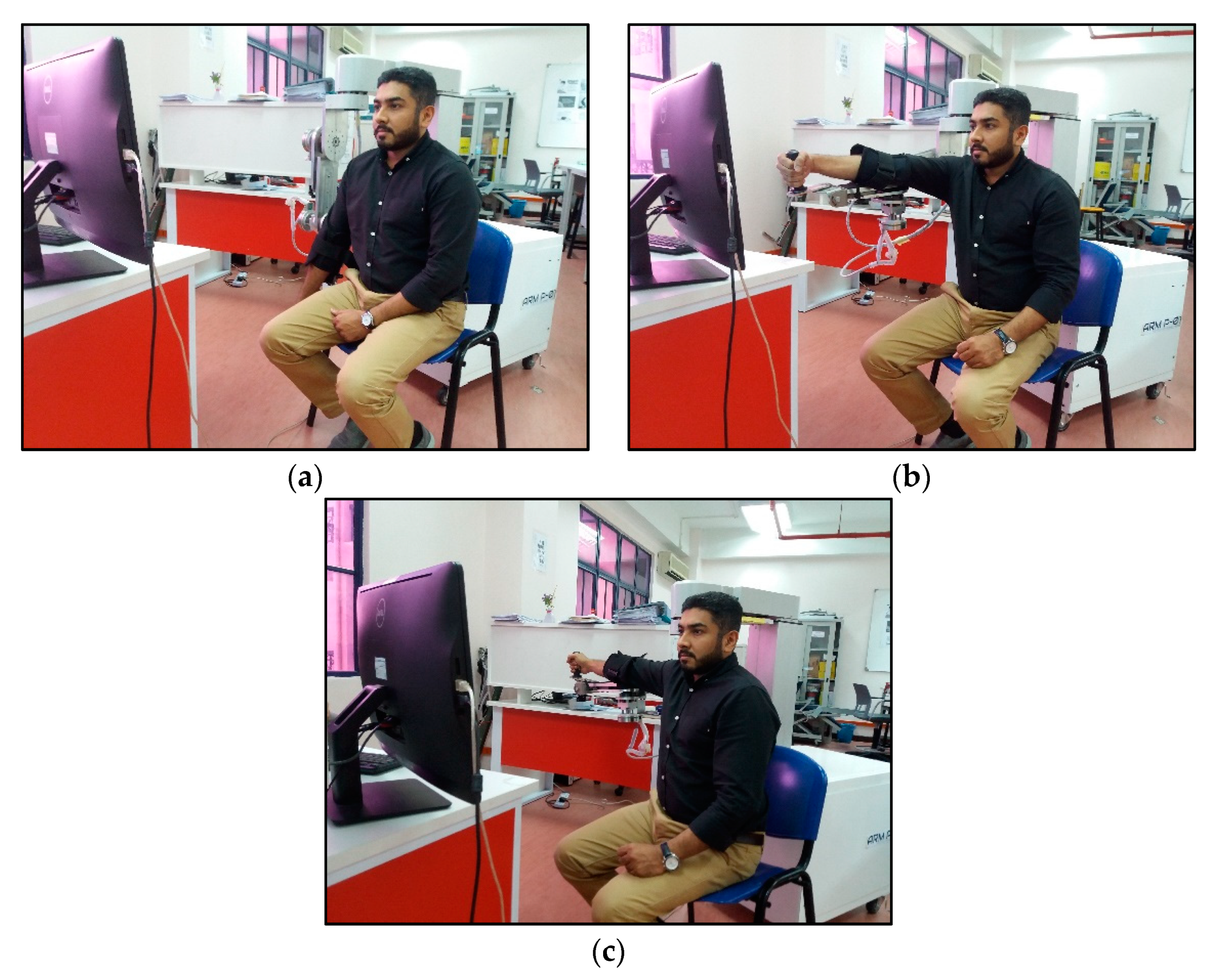
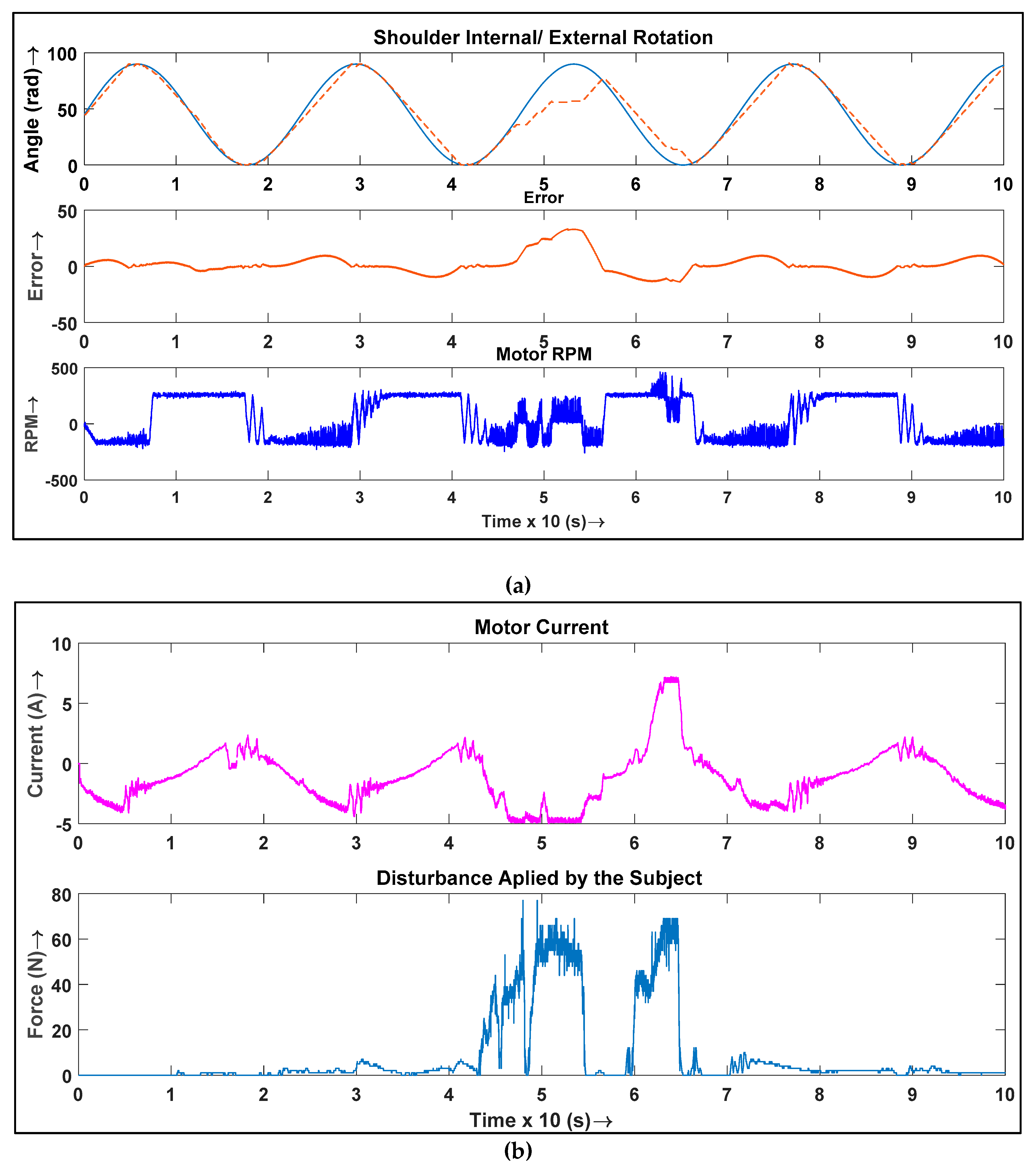
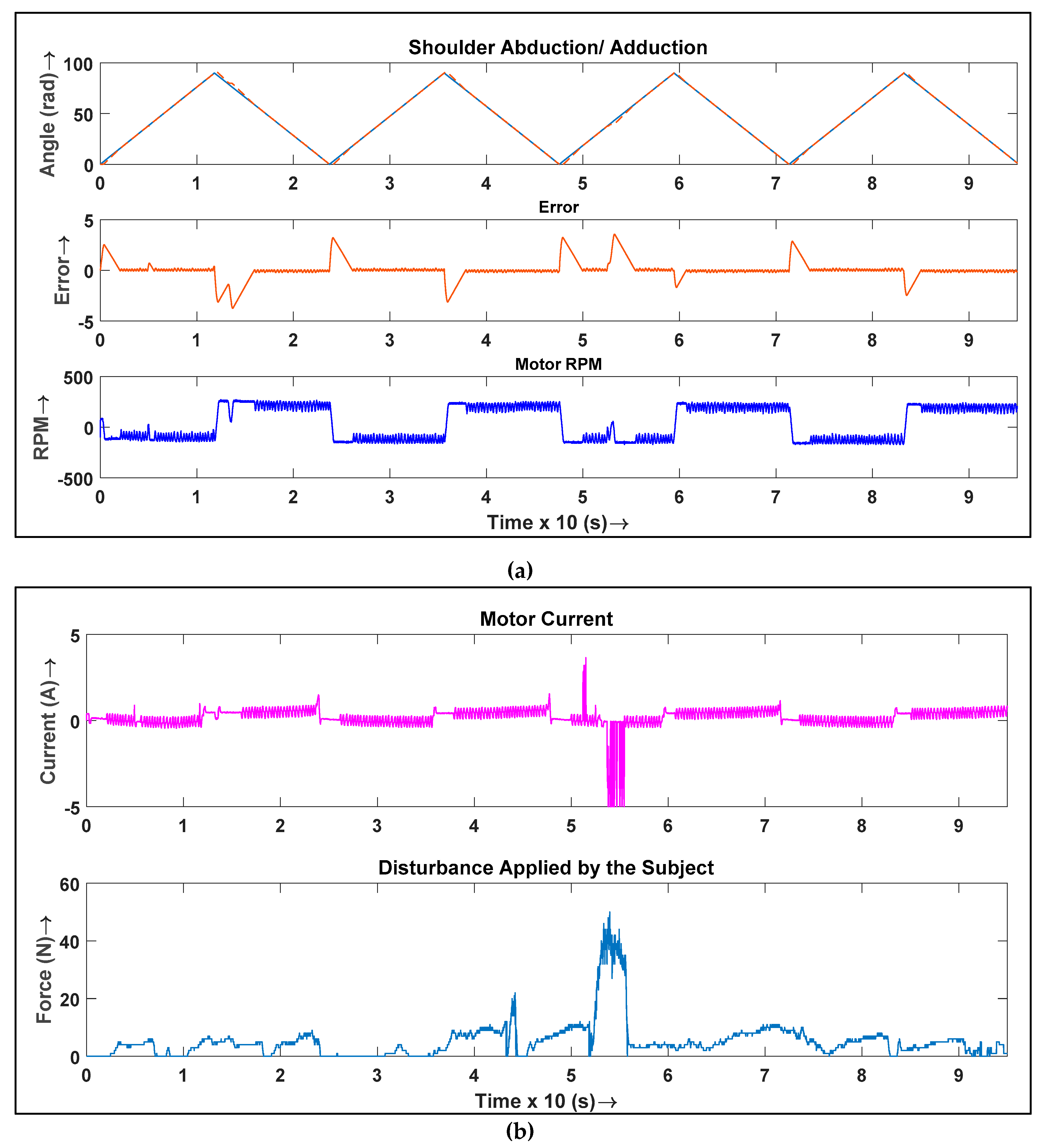
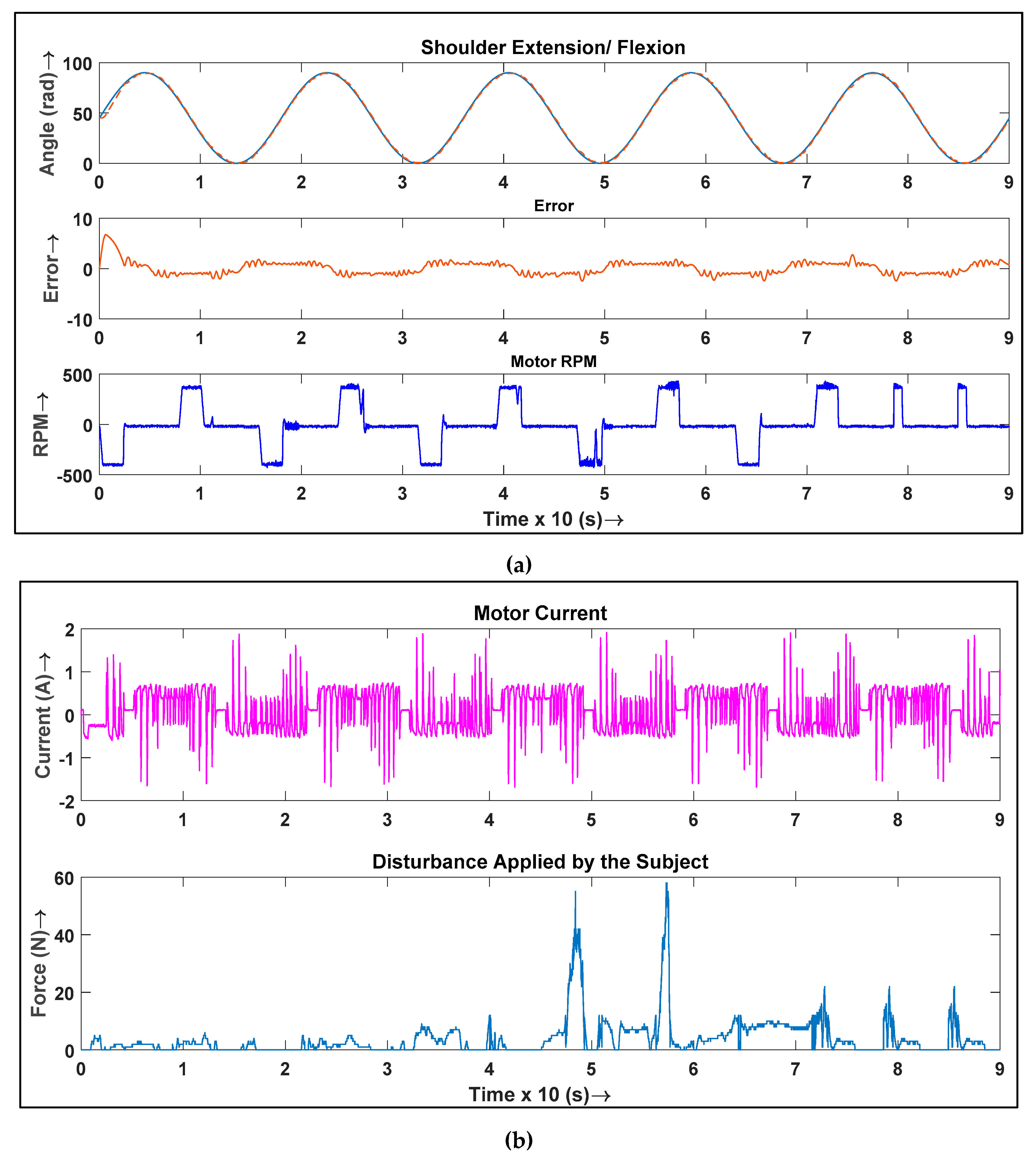
Rehabilitation robotics have been studied for decades, but few researchers have ever considered using optimization techniques for gait training. This paper presents PSO- and ABC-based tuning techniques for a 2-DOF PID controller used in the robot controlling trajectories of different exercise movements performed by the shoulder joints, namely internal/external rotation, abduction/adduction, and extension/flexion. RAX-1 was used as a mechanical experimental platform. The control parameters of the PID controller were tuned using the ABC and PSO algorithms as well as the Zeigler-Nichols method. The simulation results demonstrated better feasibility of the proposed controller in terms of robustness. An ABC-optimized PID controller was also implemented into the hardware for three subjects, with each performing different exercises. It was necessary for the robot to perform steady motion with no steady state error during the process of rehabilitation, as any abrupt movement could dislocate the shoulder joint. The hardware results showed that the controller could trace the desired trajectory with a very minute overshoot in the response and significantly low response times, which are desirable in rehabilitation. Finally, this study compared the performance of PID controllers optimized with ABC and the Zeigler-Nichols method, respectively. The controller tuned using the Zeigler-Nichols method demonstrated a decent rise time but large overshoot in the response, which is dangerous for rehabilitation applications. However, the hardware response of the system had less overshoot and no steady-state error when the ABC optimizer was used to tune the PID parameters. In summary, this study focused on finding optimal parameters of the PID controller used in an upper limb rehabilitation robotic system. In the future, we plan to broaden the spectrum of this study by incorporating various protocols related to the elbow and wrist rehabilitation with an updated mechanical structure. Analysis with other notable optimization techniques such as firefly and ant colony algorithms will be further investigated to compare their parameters and validate their capabilities in rehabilitation applications.

References

1. Page, S.J.; Levine, P.; Leonard, A.C. Modified constraint-induced therapy in acute stroke: A randomized controlled pilot study. Neurorehabilit. Neural Repair 2005, 19, 27–32. [Google Scholar] [CrossRef] [PubMed]
2. Williams, G.R. Incidence and characteristics of total stroke in the United States. BMC Neurol. 2001, 1, 2. [Google Scholar] [CrossRef]
3. Members, W.G.; Go, A.S.; Mozaffarian, D.; Roger, V.L.; Benjamin, E.J.; Berry, J.D.; Blaha, M.J.; Dai, S.; Ford, E.S.; Fox, C.S. Heart disease and stroke statistics—2014 update: A report from the American Heart Association. Circulation 2014, 129, e28. [Google Scholar]
4. Bingül, Z.; Karahan, O. A Fuzzy Logic Controller tuned with PSO for 2 DOF robot trajectory control. Expert Syst. Appl. 2011, 38, 1017–1031. [Google Scholar] [CrossRef]
5. Bharat, S.; Ganguly, A.; Chatterjee, R.; Basak, B.; Sheet, D.K.; Ganguly, A. A Review on Tuning Methods for PID Controller. Asian J. Converg. Technol. 2019, 3, 17–22. [Google Scholar]
6. Ali, A.; Ahmed, S.F.; Kadir, K.A.; Joyo, M.K.; Yarooq, R.S. Fuzzy PID controller for upper limb rehabilitation robotic system. In Proceedings of the 2018 IEEE International Conference on Innovative Research and Development (ICIRD), Bangkok, Thailand, 11–12 May 2018; pp. 1–5. [Google Scholar]
7. Kudinov, Y.; Kolesnikov, V.; Pashchenko, F.; Pashchenko, A.; Papic, L. Optimization of Fuzzy PID Controller’s Parameters. Procedia Comput. Sci. 2017, 103, 618–622. [Google Scholar] [CrossRef]
8. Leng, G.; McGinnity, T.M.; Prasad, G. Design for self-organizing fuzzy neural networks based on genetic algorithms. IEEE Trans. Fuzzy Syst. 2006, 14, 755–766. [Google Scholar] [CrossRef]
9. Juang, C.-F.; Lu, C.-M.; Lo, C.; Wang, C.-Y. Ant colony optimization algorithm for fuzzy controller design and its FPGA implementation. IEEE Trans. Ind. Electron. 2008, 55, 1453–1462. [Google Scholar] [CrossRef]
10. Das, M.T.; Dulger, L.C.; Das, G.S. Robotic applications with particle swarm optimization (pso). In Proceedings of the 2013 International Conference on Control, Decision and Information Technologies (CoDIT), Hammamet, Tunisia, 6–8 May 2013; pp. 160–165. [Google Scholar]
11. Karaboga, D. An Idea Based on Honey Bee Swarm for Numerical Optimization; Technical Report-tr06; Erciyes University, Engineering Faculty, Computer Engineering Department: Kayseri, Turkey, 2005. [Google Scholar]
12. Iruthayarajan, M.W.; Baskar, S. Optimization of PID Parameters Using Genetic Algorithm and Particle Swarm Optimization; Curran Associates: New York, NY, USA, 2007. [Google Scholar]
13. Elbeltagi, E.; Hegazy, T.; Grierson, D. Comparison among five evolutionary-based optimization algorithms. Adv. Eng. Inform. 2005, 19, 43–53. [Google Scholar] [CrossRef]
14. Shen, Z.; Zhou, J.; Gao, J.; Song, R. Fuzzy Logic Based PID Control of a 3 DOF Lower Limb Rehabilitation Robot. In Proceedings of the 2018 IEEE 8th Annual International Conference on CYBER Technology in Automation, Control, and Intelligent Systems (CYBER), Tianjin, China, 9–13 July 2018; pp. 818–821. [Google Scholar]
15. Wu, J.; Huang, J.; Wang, Y.; Xing, K.; Xu, Q. Fuzzy PID control of a wearable rehabilitation robotic hand driven by pneumatic muscles. In Proceedings of the 2009 International Symposium on Micro-NanoMechatronics and Human Science, Nagoya, Japan, 8–11 November 2009; pp. 408–413. [Google Scholar]
16. Wu, J.; Wang, Y.; Huang, J.; Xing, K. Artificial Bee Colony algorithm based Auto-Disturbance Rejection Control for rehabilitation robotic arm driven by PM-TS actuator. In Proceedings of the 2012 International Conference on Modelling, Identification & Control (ICMIC), Hubei, China, 24–26 June 2012; pp. 802–807. [Google Scholar]
17. Tarmizi, W.F.W.; Elamvazuthi, I.; Perumal, N.; Nurhanim, K.; Khan, M.A.; Parasuraman, S.; Nandedkar, A. A Particle Swarm Optimization-PID controller of a DC Servomotor for Multi-Fingered Robot Hand. In Proceedings of the 2016 2nd IEEE International Symposium on Robotics and Manufacturing Automation (ROMA), Ipoh, Malaysia, 25–27 September 2016; pp. 1–6. [Google Scholar]
18. Annisa, J.; Darus, I.M.; Tokhi, M.; Mohamaddan, S. Implementation of PID Based Controller Tuned by Evolutionary Algorithm for Double Link Flexible Robotic Manipulator. In Proceedings of the 2018 International Conference on Computational Approach in Smart Systems Design and Applications (ICASSDA), Kuching, Malaysia, 15–17 August 2018; pp. 1–5. [Google Scholar]
19. Yan, F.; Wang, Y.; Xu, W.; Chen, B. Time delay control of cable-driven manipulators with artificial bee colony algorithm. Trans. Can. Soc. Mech. Eng. 2018, 42, 177–186. [Google Scholar] [CrossRef]
20. Bingul, Z.; Karahan, O. Comparison of PID and FOPID controllers tuned by PSO and ABC algorithms for unstable and integrating systems with time delay. Optim. Control Appl. Methods 2018, 39, 1431–1450. [Google Scholar] [CrossRef]
21. Begum, K.G.; Rao, A.S.; Radhakrishnan, T. Maximum sensitivity based analytical tuning rules for PID controllers for unstable dead time processes. Chem. Eng. Res. Des. 2016, 109, 593–606. [Google Scholar] [CrossRef]
22. Biodex, Manual, System 3 and 4 Upper Extremity Hemiparetic Attachments—Operation. Available online: https://www.biodex.com/physical-medicine/products/dynamometers/system-4-accessories/ue-hemiparetic-attachments (accessed on 3 December 2018).
23. Shah, J.A.; Rattan, S.; Nakra, B. End-effector position analysis using forward kinematics for 5 DOF pravak robot arm. IAES Int. J. Robot. Autom. 2013, 2, 112. [Google Scholar] [CrossRef]
24. Lai, L.-C.; Chang, Y.-C.; Jeng, J.-T.; Huang, G.-M.; Li, W.-N.; Zhang, Y.-S. A PSO method for optimal design of PID controller in motion planning of a mobile robot. In Proceedings of the 2013 International Conference on Fuzzy Theory and Its Applications (iFUZZY), Taipei, Taiwan, 6–8 December 2013; pp. 134–139. [Google Scholar]
25. Yousof, Z.M.; Billah, M.M.; Joyo, K.M.; Kadir, K.; Qisti, M. Milestone 5 Report: Robotic System Development, Integration and Testing Product Testing; Under the Project of Building Our Robotic Competitiveness in Medical Healthcare: Development of Robot for Assisted Recovery and Rehabilitation; Technology Park Malaysia Engineering Sdn Bhd: Kuala Lumpur, Malaysia, 2018. [Google Scholar]
26. Czarkowski, D.; O’Mahony, T. Intelligent controller design based on gain and phase margin specifications. In Proceedings of the Irish Signals and Systems Conference 2004, Belfast, Ireland, 30 June–2 July 2004. [Google Scholar]
27. Aouf, A.; Boussaid, L.; Sakly, A. A PSO algorithm applied to a PID controller for motion mobile robot in a complex dynamic environment. In Proceedings of the 2017 International Conference on Engineering & MIS (ICEMIS), Monastir, Tunisia, 8–10 May 2017; pp. 1–7. [Google Scholar]
28. Karaboga, D.; Basturk, B. On the performance of artificial bee colony (ABC) algorithm. Appl. Soft Comput. 2008, 8, 687–697. [Google Scholar] [CrossRef]
29. Kumar, A.; Kumar, D.; Jarial, S. A Review on Artificial Bee Colony Algorithms and Their Applications to Data Clustering. Cybern. Inf. Technol. 2017, 17, 3–28. [Google Scholar] [CrossRef] [Green Version]
30. Mustafa, A.M.; Al-Saif, A. Modeling, simulation and control of 2-R robot. Glob. J. Res. Eng. 2014, 14, 49–54. [Google Scholar]
31. Naidu, K.; Mokhlis, H.; Bakar, A.A. Multiobjective optimization using weighted sum artificial bee colony algorithm for load frequency control. Int. J. Electr. Power Energy Syst. 2014, 55, 657–667. [Google Scholar] [CrossRef]
Figure 1. (a) Shoulder abduction and adduction, (b) Shoulder Extension/Flexion, (c) Shoulder External and Internal rotation [22].
Electronics 08 00826 g001aElectronics 08 00826 g001b
Figure 2. 3D CAD Model of Robot.
Electronics 08 00826 g002
Figure 3. (a) DH convention for frame assignment, (b) Kinematics of the Robotic Arm.
Electronics 08 00826 g003
Figure 4. Internal model of DC motor.
Electronics 08 00826 g004
Figure 5. RAX-1 Mechanical design.
Electronics 08 00826 g005
Figure 6. (a) HMI displaying rehabilitation training modes, (b) HMI displaying selection for shoulder exercise, (c) System Block Diagram.
Electronics 08 00826 g006aElectronics 08 00826 g006b
Figure 7. Controller Board.
Electronics 08 00826 g007
Figure 8. 2-DOF PID block diagram.
Electronics 08 00826 g008
Figure 9. PSO Optimization Flow.
Electronics 08 00826 g009
Figure 10. ABC Optimization Flow.
Electronics 08 00826 g010
Figure 11. General Structure of the proposed control System Diagram.
Electronics 08 00826 g011
Figure 12. Step response of Joint 1 using ISE, IAE, ITSE and ITAE.
Electronics 08 00826 g012
Figure 13. Step response of Joint 2 using ISE, IAE, ITSE and ITAE.
Electronics 08 00826 g013
Figure 14. Nyquist plot for closed loop system of joint 1 and joint 2.
Electronics 08 00826 g014
Figure 15. A subject performing exercise with assistance of exoskeleton device.
Electronics 08 00826 g015
Figure 16. (a) Shoulder Internal/External Rotation, (b) Current driven from the motor and Disturbance applied by first subject.
Electronics 08 00826 g016
Figure 17. (a) Shoulder Abduction/ Adduction, (b) Current driven from the motor and Disturbance applied by second subject.
Electronics 08 00826 g017
Figure 18. (a) Shoulder Extension/Flexion, (b) Current driven from the motor and Disturbance applied by third subject.
Electronics 08 00826 g018
Figure 19. (a) Response of the system with ABC optimized PID and tuned using Zeigler-Nichols, (b) Error of the system with ABC optimized PID and tuned using Zeigler-Nichols.
Electronics 08 00826 g019