Multisensor RFS Filters for Unknown and Changing Detection Probability


Abstract
1. Introduction
2. Background
2.1. Multisensor Measurement Partitioning
2.2. The MS-CPHD Filter
2.3. The MS-MeMBer Filter
2.4. The IGGM Model
3. Multisensor Filters Based on IGGM Model
3.1. The IGGM-MS-CPHD Filter
3.1.1. Prediction
3.1.2. Update
3.2. The IGGM-MS-MeMBer Filter
3.2.1. Prediction
3.2.2. Update
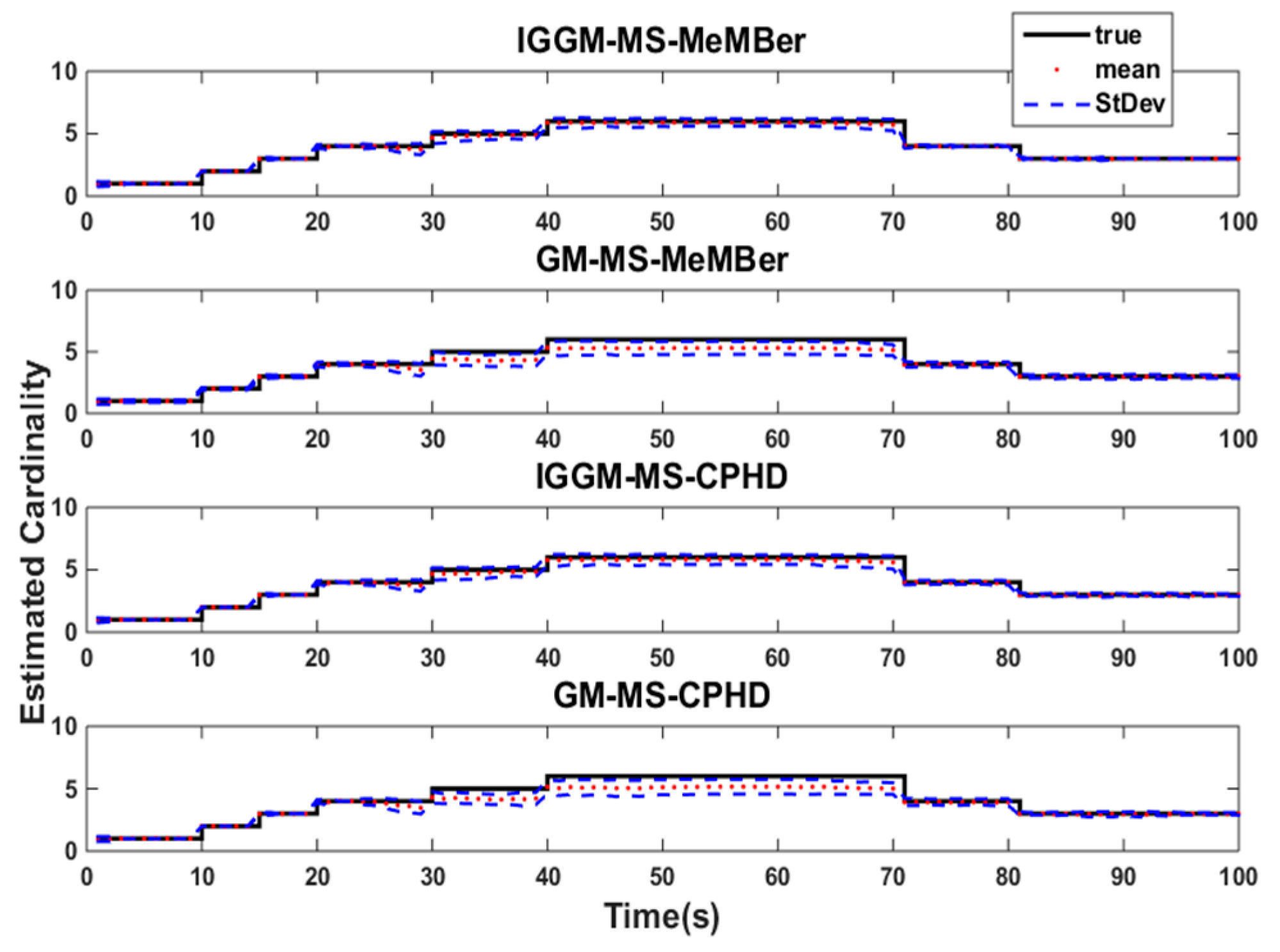
4. Simulation Results and Analysis
4.1. System Model
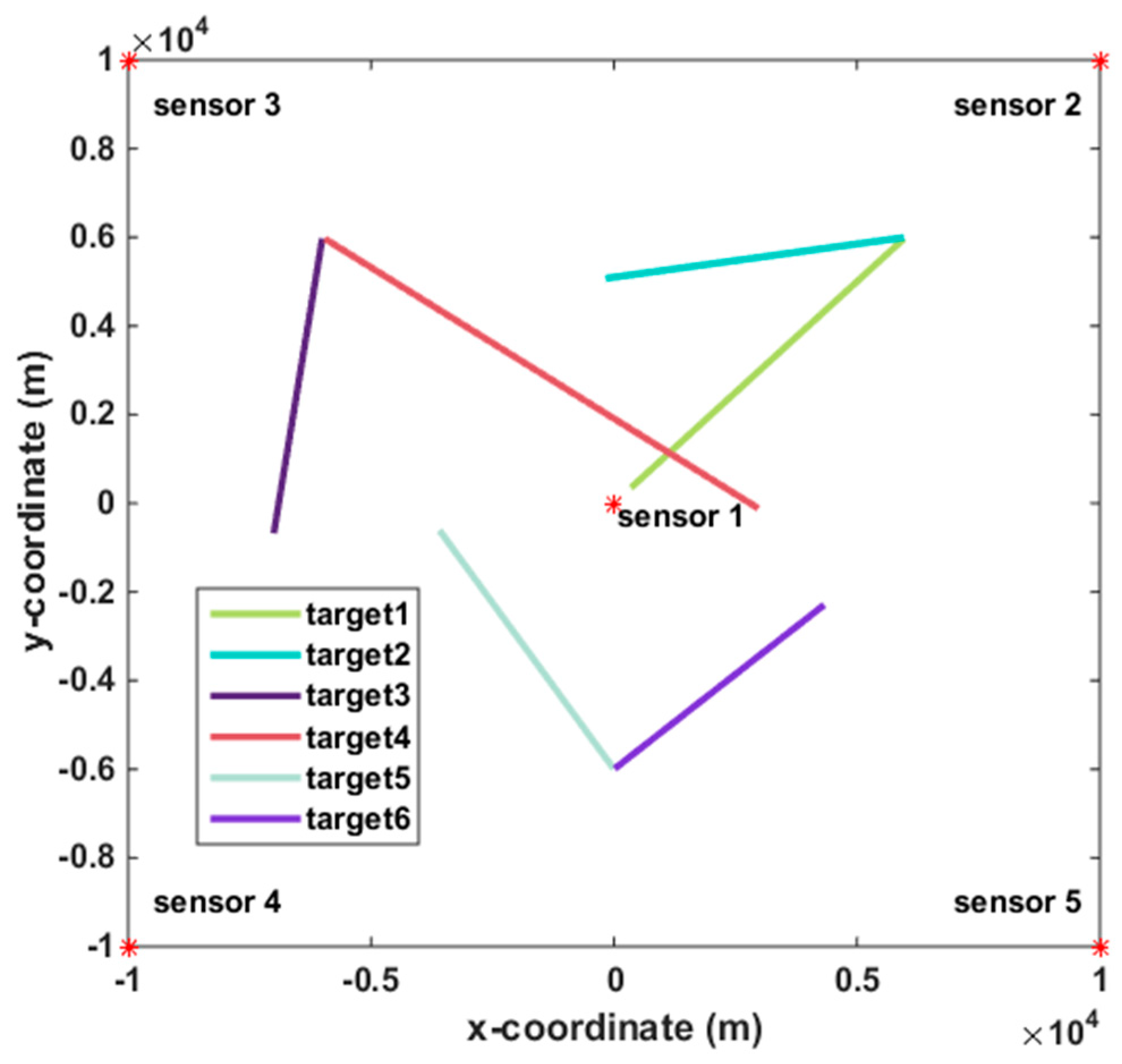
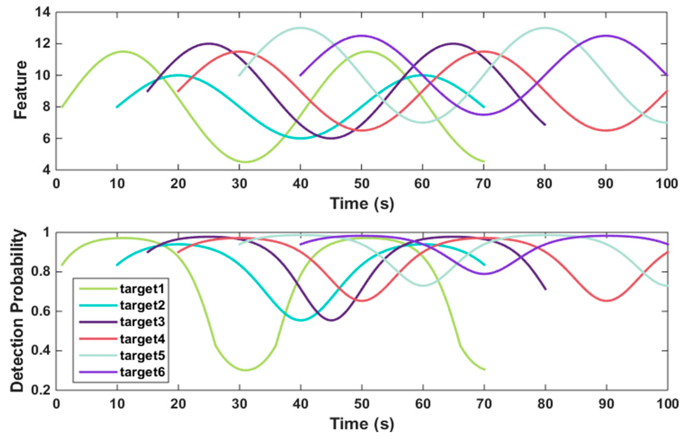
4.2. Simulation 1
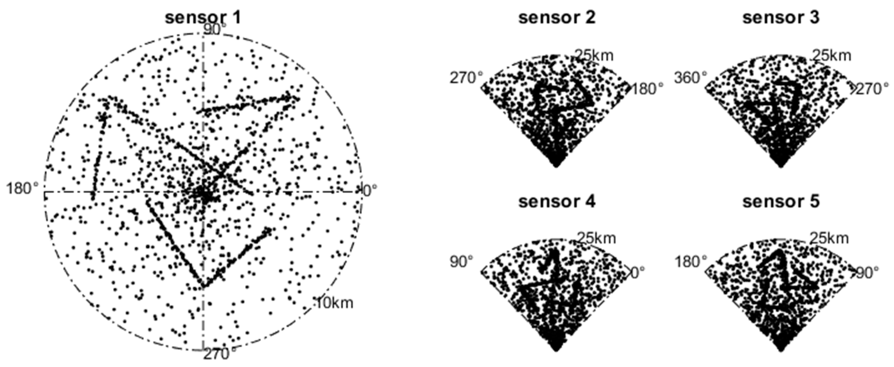
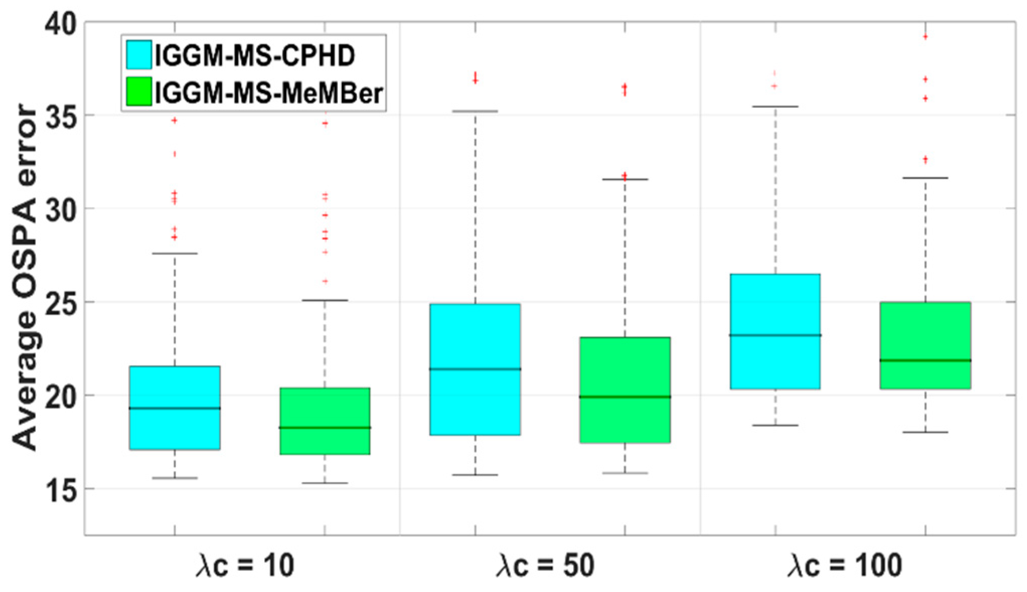
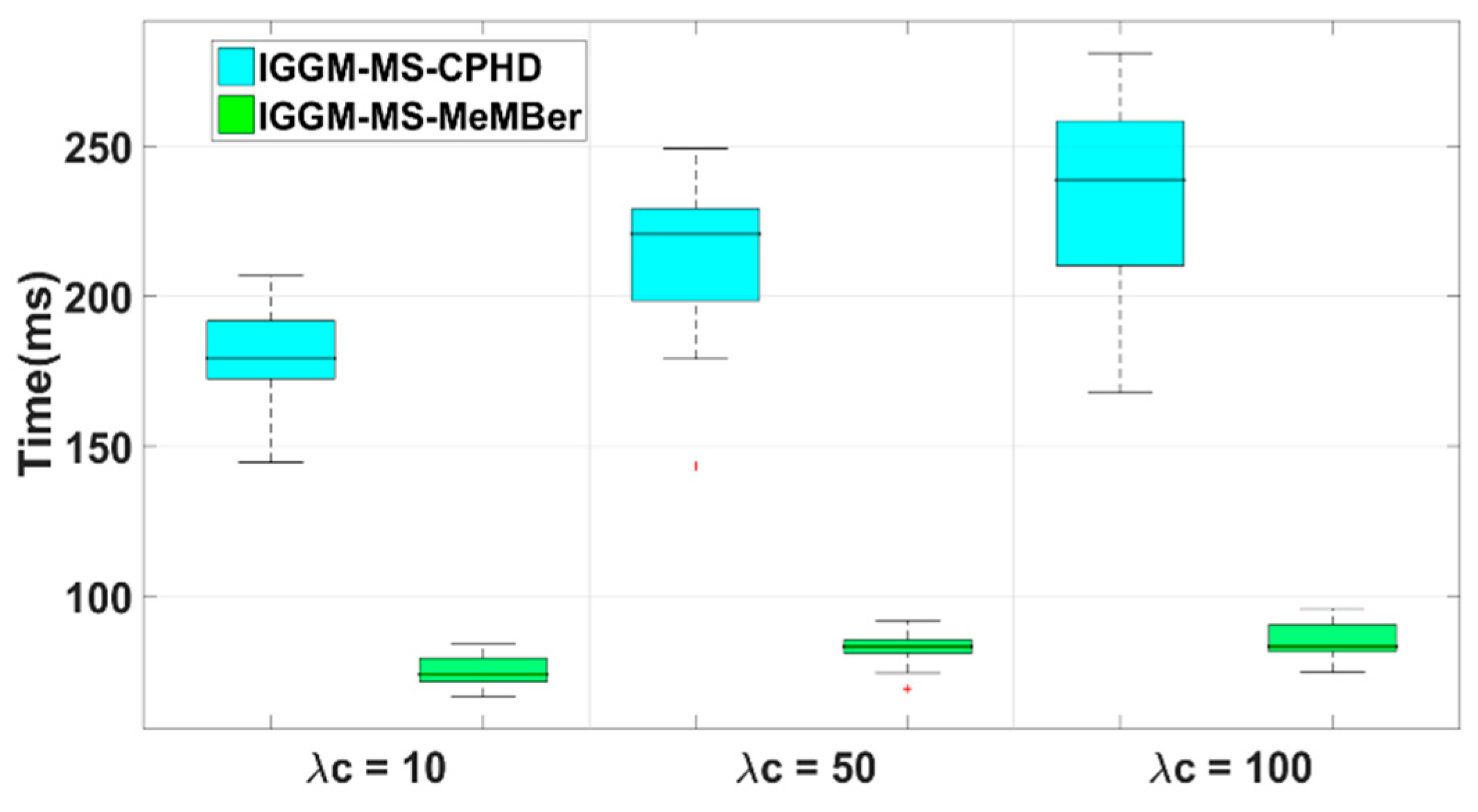
4.3. Simulation 2
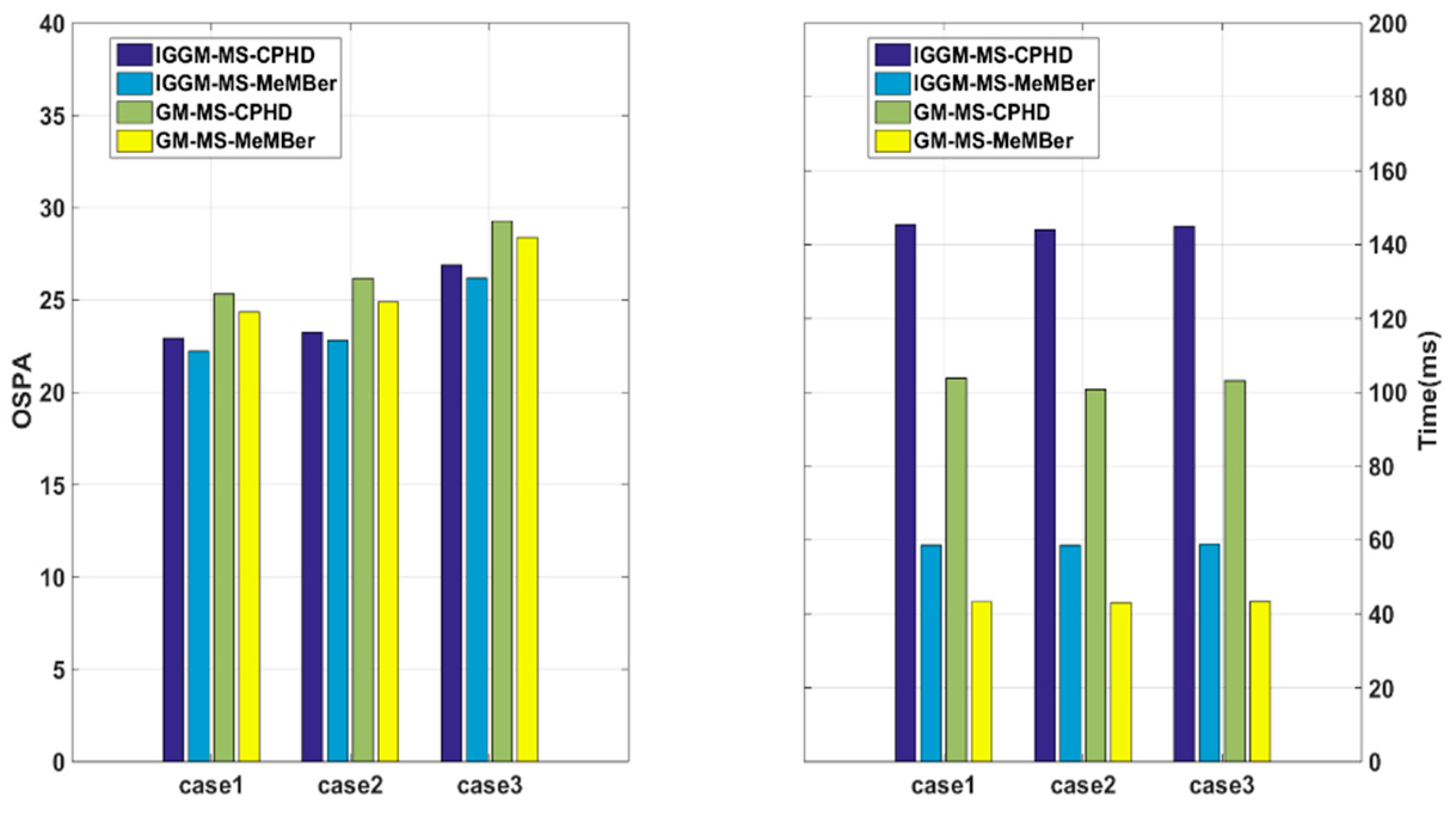
- Case 1: assume that the four sensors are located at [−10 km, 10 km], [−10 km, −10 km], [10 km, −10 km], and [10 km, 10 km], respectively;
- Case 2: assume that the four sensors are located at [−10 km, 0 km], [0 km, −10 km], [10 km, 0 km], and [0 km, 10 km], respectively;
- Case 3: assume that the four sensors are located at [−9 km, −10 km], [−3 km, −10 km], [3 km, −10 km], and [9 km, −10 km], respectively.
5. Conclusions
Author Contributions
Funding
Conflicts of Interest
References
- Mahler, R.P.S. Advances in Statistical Multisource-Multitarget Information Fusion; Artech House: Norwood, MA, USA, 2014. [Google Scholar]
- Quan, H.W.; Li, J.H.; Peng, D.L. Multi-target Tracking Based on Random Set Theory. Fire Control Command Control 2015, 40, 49–56. [Google Scholar]
- Shen, T.H.; Xue, A.K.; Zhou, Z.L. Multi-sensor Gaussian Mixture PHD Fusion for Multi-target Tracking. Acta Autom. Sin. 2017, 43, 1028–1037. [Google Scholar]
- Reid, D. An algorithm for tracking multiple targets. IEEE Trans. Autom. Control 1979, 24, 843–854. [Google Scholar] [CrossRef]
- Kirubarajan, T.; Bar-Shalom, Y. Probabilistic data association techniques for target tracking in clutter. Proc. IEEE 2004, 92, 536–557. [Google Scholar] [CrossRef]
- Mahler, R.P.S. Statistical Multisource-Multitarget Information Fusion; Artech House: Norwood, MA, USA, 2007. [Google Scholar]
- Vo, B.N.; Ma, W.K. The Gaussian Mixture Probability Hypothesis Density Filter. IEEE Trans. Signal Process. 2006, 54, 4091–4104. [Google Scholar] [CrossRef]
- Vo, B.T.; Vo, B.N.; Cantoni, A. Analytic Implementations of the Cardinalized Probability Hypothesis Density Filter. IEEE Trans. Signal Process. 2007, 55, 3553–3567. [Google Scholar] [CrossRef]
- Vo, B.T.; Vo, B.N.; Cantoni, A. On multi-Bernoulli approximations to the Bayes multi-target filter. In Proceedings of the International Colloquium on Information Fusion, Xi’an, China, 22–25 August 2007. [Google Scholar]
- Vo, B.T.; Vo, B.N.; Cantoni, A. The Cardinality Balanced Multi-Target Multi-Bernoulli Filter and Its Implementations. IEEE Trans. Signal Process. 2009, 57, 409–423. [Google Scholar]
- Vo, B.T.; Vo, B.N. Labeled random finite sets and multi-object conjugate priors. IEEE Trans. Signal Process. 2013, 61, 3460–3475. [Google Scholar] [CrossRef]
- Reuter, S.; Vo, B.T.; Vo, B.N.; Dietmayer, K. The labeled multi-Bernoulli filter. IEEE Trans. Signal Process. 2014, 62, 3246–3260. [Google Scholar]
- Fantacci, C.; Vo, B.T.; Papi, F.; Vo, B.N. The Marginalized delta-GLMB Filter. arXiv 2015, arXiv:1501.00926. [Google Scholar]
- Mertens, M.; Ulmke, M. Ground moving target tracking using signal strength measurements with the GM-CPHD filter. In Proceedings of the 2012 Workshop on Sensor Data Fusion: Trends, Solutions, Applications (SDF), Bonn, Germany, 4–6 September 2012. [Google Scholar]
- Maggio, E.; Taj, M.; Cavallaro, A. Efficient Multitarget Visual Tracking Using Random Finite Sets. IEEE Trans. Circuits Syst. Video Technol. 2008, 18, 1016–1027. [Google Scholar] [CrossRef]
- Kim, D.Y.; Jeon, M. Robust multi-Bernoulli filtering for visual tracking. In Proceedings of the International Conference on Control, Automation and Information Sciences (ICCAIS 2014), Gwangju, Korea, 2–5 December 2014; pp. 47–51. [Google Scholar]
- Mahler, R.P.S. The multisensor PHD filter: I. General solution via multitarget calculus. Proc. Spie Int. Soc. Opt. Eng. 2009, 7336. [Google Scholar]
- Delande, E.; Duflos, E.; Heurguier, D.; Vanheeghe, P. Multi-Target PHD Filtering: Proposition of Extensions to the Multi-Sensor Case; Research Report RR-7337; HAL-INRIA: Le Chesnay, French, 2010; p. 64. [Google Scholar]
- Mahler, R.P.S. The multisensor PHD filter: II. Erroneous solution via Poisson magic. In Proceedings of the SPIE International Conference on Signal Processing, Sensor Fusion, Target Recognition, Orlando, FL, USA, 13–17 April 2009. [Google Scholar]
- Mahler, R.P.S. Approximate multisensor CPHD and PHD filters. In Proceedings of the International Conference on Information Fusion, Edinburgh, UK, 26–29 July 2010. [Google Scholar]
- Nannuru, S.; Blouin, S.; Coates, M.; Rabbat, M. Multisensor CPHD filter. IEEE Trans. Aerosp. Electron. Syst. 2016, 52, 1834–1854. [Google Scholar] [CrossRef]
- Saucan, A.A.; Coates, M.J.; Rabbat, M. A Multisensor Multi-Bernoulli Filter. IEEE Trans. Signal Process. 2017, 65, 5495–5509. [Google Scholar] [CrossRef]
- Wei, B.; Nener, B.; Liu, W.; Ma, L. Centralized multi-sensor multi-target tracking with labeled random finite sets. In Proceedings of the International Conference on Control, Automation and Information Sciences (ICCAIS), Ansan, Korea, 27–29 October 2016. [Google Scholar]
- Ren, X.Y. A Novel Multiple Target Tracking Algorithm and Its Evaluation; Graduate University of Chinese Academy of Sciences: Beijing, China, May 2012. [Google Scholar]
- Mahler, R.P.S.; Vo, B.T.; Vo, B.N. CPHD filtering with unknown clutter rate and detection profile. IEEE Trans. Signal Process. 2011, 59, 3497–3513. [Google Scholar] [CrossRef]
- Vo, B.T.; Vo, B.N.; Hoseinnezhad, R.; Mahler, R.P.S. Multi-Bernoulli filtering with unknown clutter intensity and sensor field-of-view. In Proceedings of the 45th Annual Conference on Information Sciences and Systems (CISS), Baltimore, MD, USA, 23–25 March 2011. [Google Scholar]
- Vo, B.T.; Vo, B.N.; Hoseinnezhad, R.; Mahler, R.P.S. Robust Multi-Bernoulli filtering. IEEE J. Sel. Top. Signal Process. 2013, 7, 399–409. [Google Scholar] [CrossRef]
- Punchihewa, Y.; Vo, B.T.; Vo, B.N.; Kim, D.Y. Multiple Object Tracking in Unknown Backgrounds with Labeled Random Finite Sets. IEEE Trans. Signal Process. 2017, 66, 3040–3055. [Google Scholar] [CrossRef]
- Li, C.; Wang, W.; Kirubarajan, T.; Sun, J.; Lei, P. PHD and CPHD Filtering with Unknown Detection Probability. IEEE Trans. Signal Process. 2018, 66, 3784–3798. [Google Scholar] [CrossRef]
- Qian, K.; Zhou, H.; Qin, H.; Rong, S.; Zhao, D.; Du, J. Guided filter and convolutional network based tracking for infrared dim moving target. Infrared Phys. Technol. 2017, 85, 431–442. [Google Scholar] [CrossRef]
- Lerro, D.; Bar-Shalom, Y. Automated Tracking with Target Amplitude Information. In Proceedings of the American Control Conference, San Diego, CA, USA, 23–25 May 1990; pp. 2875–2880. [Google Scholar]
- Clark, D.; Ristic, B.; Vo, B.N.; Vo, B.T. Bayesian Multi-Object Filtering With Amplitude Feature Likelihood for Unknown Object SNR. IEEE Trans. Signal Process. 2010, 58, 26–37. [Google Scholar] [CrossRef]
- Skolnik, M. Radar Handbook, 3rd ed.; McGraw-Hill: New York, NY, USA, 2008. [Google Scholar]
- Schuhmacher, D.; Vo, B.T.; Vo, B.N. A consistent metric for performance evaluation of multi-object filters. IEEE Trans. Signal Process. 2008, 56, 3447–3457. [Google Scholar] [CrossRef]
- Grewal, M.S.; Andrews, A.P. Kalman Filtering: Theory and Practice Using MATLAB, 3rd ed.; Wiley: Hoboken, NJ, USA, 2008. [Google Scholar]


| Target | u | v | Survival Time (s) | |
|---|---|---|---|---|
| 1 | [6000, −80, 6000, −80]T | 51 | 400 | [1 70] |
| 2 | [6000, −100, 6000, −15]T | 51 | 400 | [10 70] |
| 3 | [−6000, −15, 6000, −100]T | 41 | 360 | [15 80] |
| 4 | [−6000, 110, 6000, −75]T | 41 | 360 | [20 100] |
| 5 | [0, −50, −6000, 75]T | 51 | 500 | [30 100] |
| 6 | [0, 70, −6000, 60]T | 51 | 500 | [40 100] |
| Sensor | Range r | Bearing θ |
|---|---|---|
| 1 | 0–10 km | 0–360° |
| 2 | 0–25 km | 180–270° |
| 3 | 0–25 km | 270–360° |
| 4 | 0–25 km | 0–90° |
| 5 | 0–25 km | 90–180° |
| IGGM-MS-CPHD | IGGM-MS-MeMBer | GM-MS-CPHD | GM-MS-MeMBer |
|---|---|---|---|
| 180 ms | 75 ms | 127 ms | 58 ms |
© 2019 by the authors. Licensee MDPI, Basel, Switzerland. This article is an open access article distributed under the terms and conditions of the Creative Commons Attribution (CC BY) license (http://creativecommons.org/licenses/by/4.0/).
Share and Cite
Zhang, Z.; Li, Q.; Sun, J. Multisensor RFS Filters for Unknown and Changing Detection Probability. Electronics 2019, 8, 741. https://doi.org/10.3390/electronics8070741
Zhang Z, Li Q, Sun J. Multisensor RFS Filters for Unknown and Changing Detection Probability. Electronics. 2019; 8(7):741. https://doi.org/10.3390/electronics8070741
Chicago/Turabian StyleZhang, Zhiguo, Qing Li, and Jinping Sun. 2019. "Multisensor RFS Filters for Unknown and Changing Detection Probability" Electronics 8, no. 7: 741. https://doi.org/10.3390/electronics8070741
APA StyleZhang, Z., Li, Q., & Sun, J. (2019). Multisensor RFS Filters for Unknown and Changing Detection Probability. Electronics, 8(7), 741. https://doi.org/10.3390/electronics8070741