Risk-Based Decision Methods for Vehicular Networks

Abstract

Vehicular networks play a key role in building intelligent transport systems for smart cities. For the purpose of achieving traffic efficiency, road safety, and traveler comfort, vehicles communicate and collaborate with each other as well as with the fixed infrastructure. In practice, not all vehicles are trustworthy. A faulty or malicious vehicle may forward or share inaccurate or bogus information, which may cause adverse things, such as, road accidents and traffic congestion. Therefore, it is very important to evaluate risk before a vehicle takes any decision. Various risk-based decision systems have already been proposed in the literature. The fuzzy risk-based decision model of vehicular networks is one of them. In this paper, we have proposed various extensions in the fuzzy risk-based decision model to achieve higher robustness, reliability, and completeness. We have presented the theoretical and simulation-based analysis and evaluation of the proposed scheme in a comprehensive manner. In addition, we have analytically cross verified the theoretical and simulation-based results. Qualitative comparison of the proposed scheme has also been presented in this work.

1. Introduction

Vehicular networks play a key role in building intelligent transport systems for smart cities. For the purpose of achieving traffic efficiency, road safety, and traveler comfort, vehicles communicate and collaborate with each other as well as with the fixed infrastructure. In practice, not all vehicles are trustworthy [1,2]. A faulty, malicious, or compromised (hacked) [3] vehicle may forward or share fake and inaccurate information, which may cause undesirable things, such as, automobile fatalities and traffic congestion. Therefore, it is highly recommended to evaluate risk before a vehicle takes any decision based on the received information from the surrounding vehicles.

According to the American Association of State Highway and Transportation Officials (AASHTO) report [4], by the end of the year 2020, most of the newly manufactured light vehicles will be able to create vehicular networks. Many automobile companies like Ford, BMW, and Toyota are prototyping VANET enabled automobiles [2,5]. The applications running on those VANET enabled vehicles will share road and traffic information with each other for the purpose of achieving traffic management efficiency. Any faulty vehicle or malicious user can jeopardize the traffic by sending fake, bogus or inaccurate information. According to the report published in 2018, “Every year, roughly 1.3 million people die in car accidents worldwide—an average of 3287 deaths per day” [6]. Therefore, it is very vital to think about risk-based decision methods that are needed for achieving high road safety.

Various risk-based decision systems [7,8,9,10,11] have already been proposed in the literature. The fuzzy risk-based decision model of vehicular networks is one of them. In this work, we present the extended version of the fuzzy-based risk decision method for vehicular networks. The initial version of this model was proposed in [12] and is briefly described in Section 2. In this model, the risk is estimated based on the three factors: (i) Vehicle contextual parameters, (ii) driver’s attitude, and (iii) application sensitivity level. The first two factors are used for threat likelihood determination, and the last parameter is used for impact derivation. In order to make this model more robust and realistic, our contribution is the following.

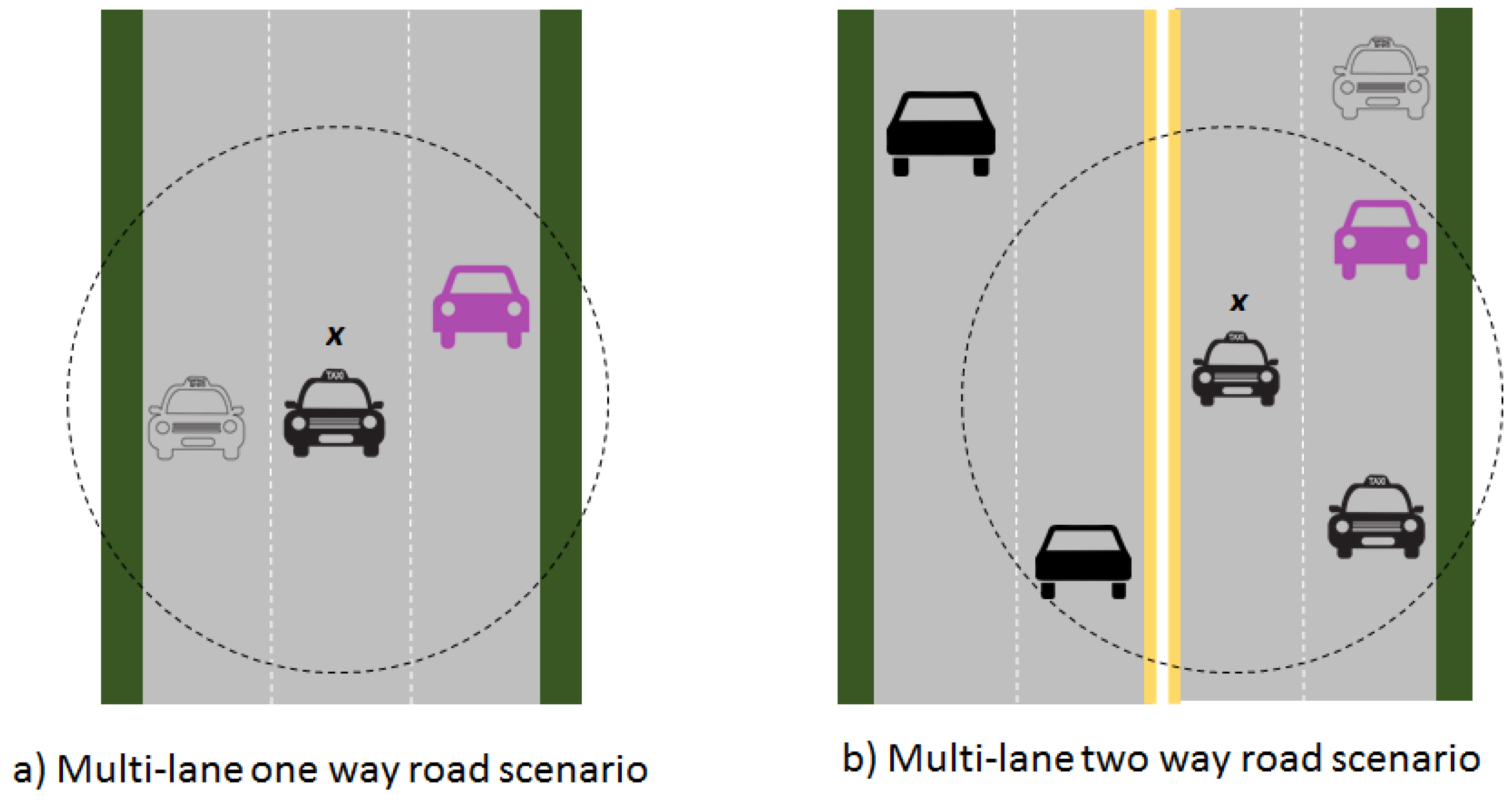
• In the earlier version, only four cases (car in front, car in rear, car on left and car on right) were considered for determining the risk from the perspective of traffic or congestion. In that model, only one case can be true at one time. This is a very simple approach. In reality, the vehicle is generally surrounded by multiple vehicles. In the extended version, we incorporated a mechanism which deals with the number of various vehicles in the surroundings (see Section 3.1).
• In the earlier version, only two cases (accelerating and decelerating) were considered for determining the risk from the perspective of speed. In many situations, the vehicle moves at a constant speed. For example, on highways, many drivers switch on the cruise control feature. In the extended version, we incorporated the case of constant speed (see Section 3.2).
• For the consistency and ease of implementation, the mapping functions of all six parameters of vehicle context is presented in the extended version (see Section 3.3).
• Vehicle context is determined based on six parameters: Lane, road, traffic, weather, speed and time. One weight value is associated with each parameter. However, the mechanism for determining the values of these weights was not presented in the earlier version. In this paper, we proposed a mechanism to calculate the weight values of the aforementioned six parameters of vehicle context (see Section 3.4).
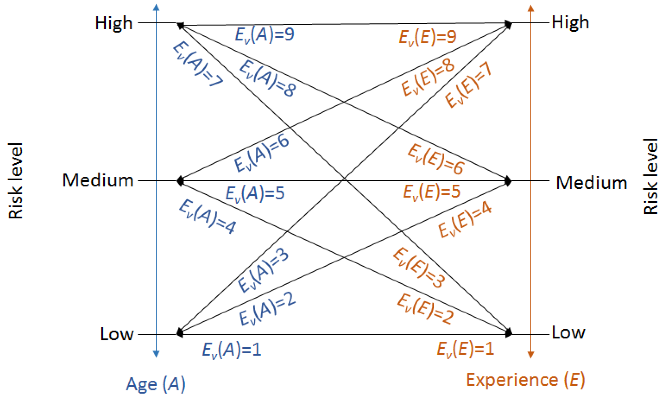
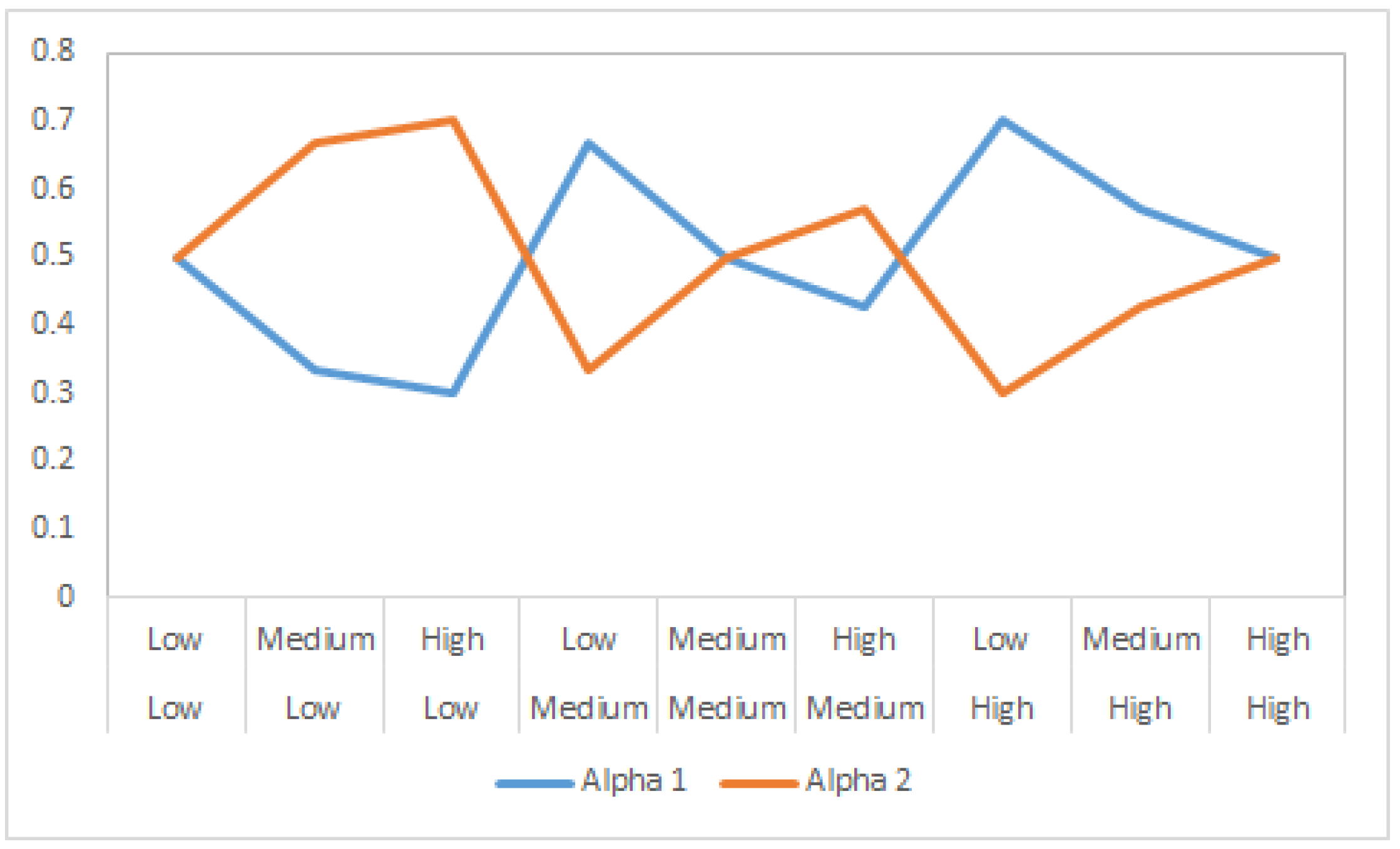
• Driver’s attitude is determined based on two factors: Age and experience. One weight value is associated with both the parameters. However, the mechanism for determining the values of these weights was also not present in the earlier version. In this paper, we proposed a mechanism to calculate the weight values of both the parameters of the driver’s attitude (see Section 3.6).
• As mentioned earlier, threat likelihood is determined based on two factors: Vehicle context and driver’s attitude. The weight values are also associated with both the factors. In this paper, we also proposed a mechanism to calculate the weight values of both the factors (see Section 3.5).
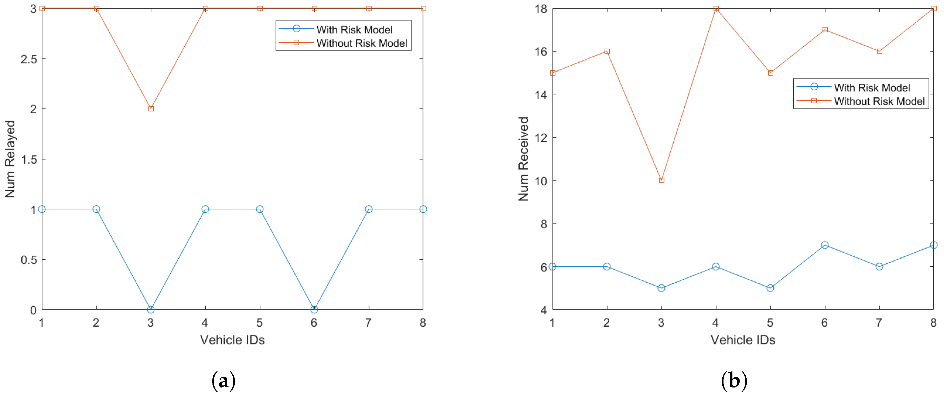
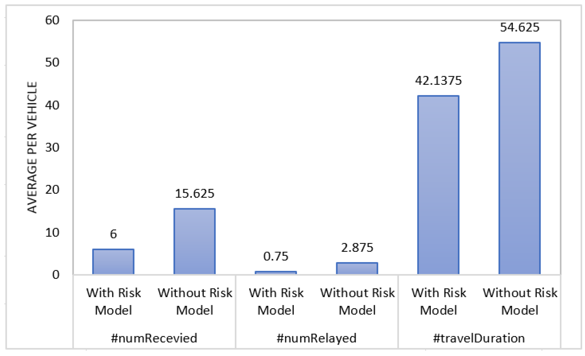
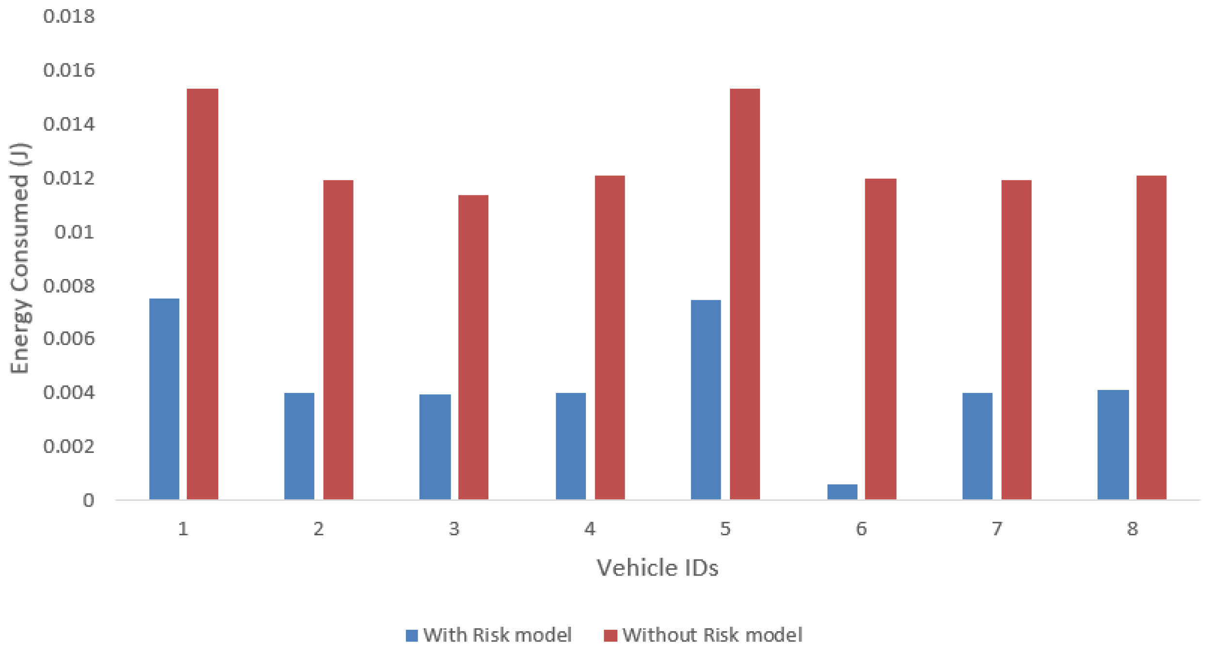
• We have provided simulation-based analysis and evaluation of proposed risk model. The results show that the proposed risk model reduces communication overhead and travel duration. As a result, fuel consumption and electricity consumption will also be reduced, which will create a positive impact on the environment and makes the vehicles eco-friendly (see Section 5).
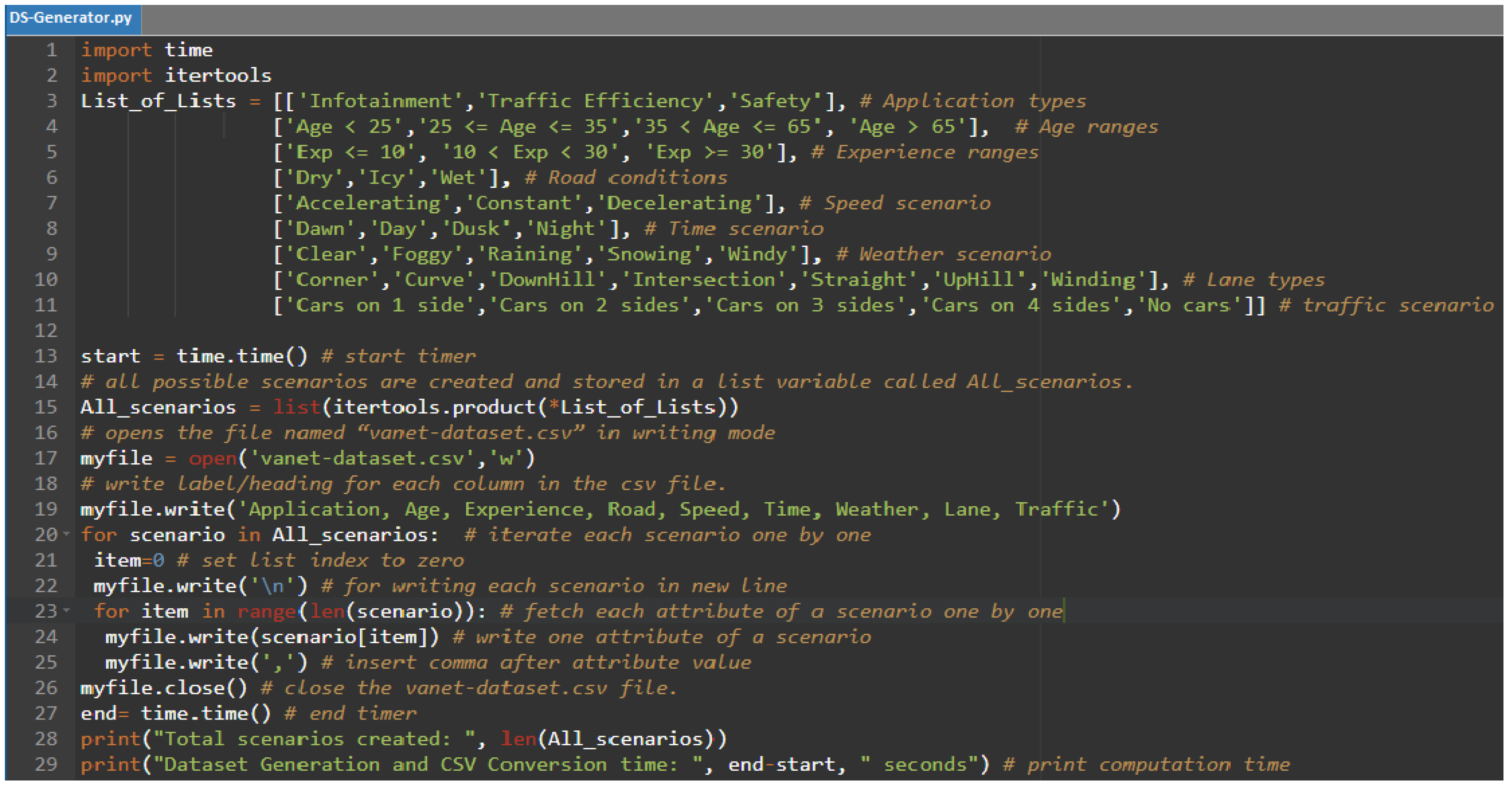
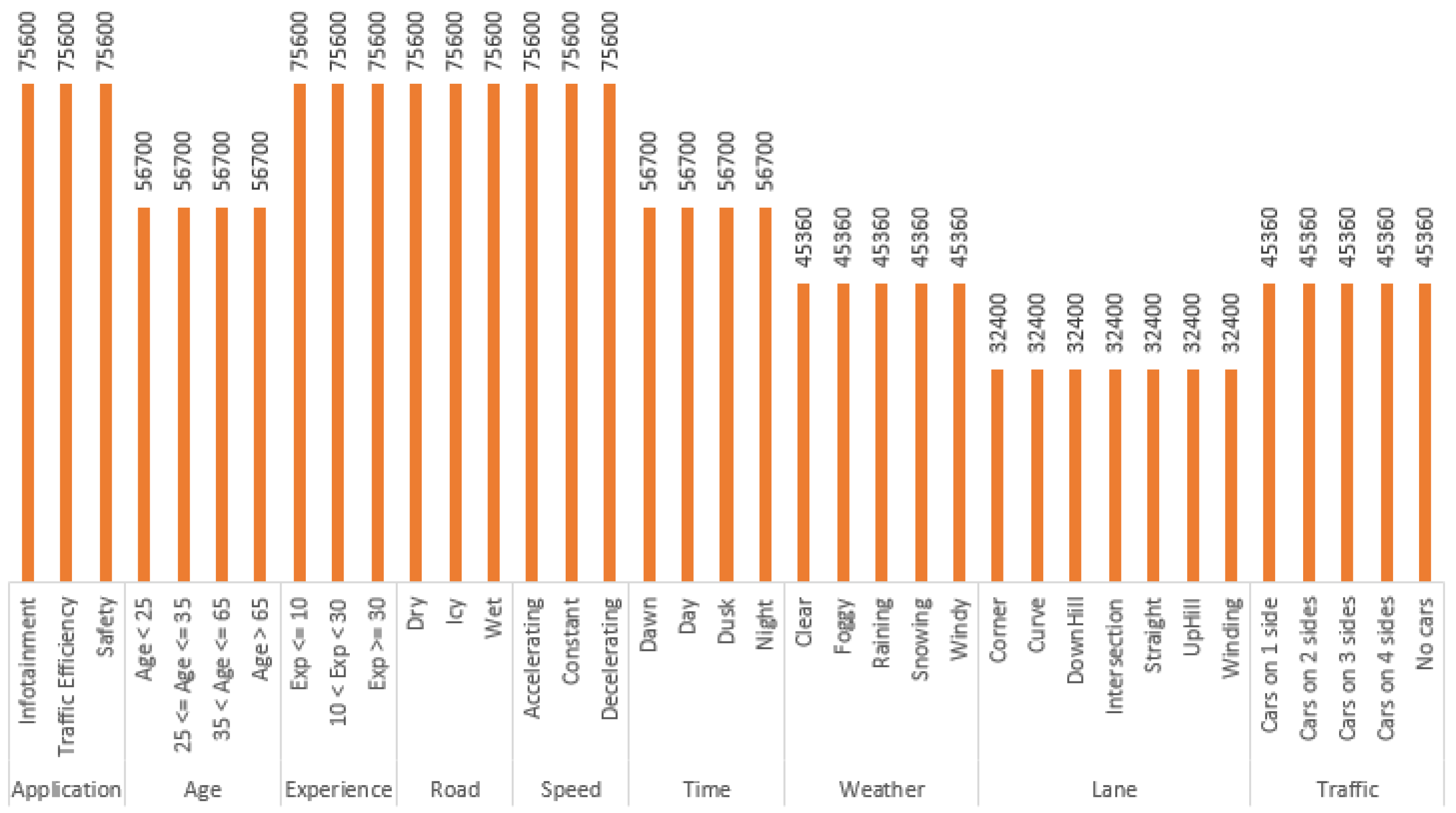
• Since simulation-based analysis and evaluation is limited in scope and does not cover all possible scenarios. Therefore, we have also conducted theoretical analysis and evaluation of the proposed method. The main problem that we faced during analysis and evaluation is the unavailability of the complete testing dataset. While some VANET datasets are available on public repositories such as TRCLC [13] provided by the Western Michigan University, those datasets do not contain various factors that we are using in our proposed model like road condition, lane type experience, etc. In order to overcome this problem, we created our own dataset generator program in python language. With the help of this program, we have created a large dataset, which contains 226,800 different scenarios.
• We have implemented the proposed model in the Python language. The program will analyze each scenario presented in the dataset and calculate risk based on the proposed method (see Section 6).
• For analytical cross-validation of the results, we have also presented mathematical proofs (see Section 4).
• Qualitative comparison of the proposed scheme is also presented in this work (see Section 7).

The rest of this paper is organized as follows. Section 2 provides a brief overview of the fuzzy risk-based decision model. Section 3 presents proposed extensions. Section 4 contains theorem and proofs. Section 5 presents simulation-based analysis and evaluation of the proposed scheme. Section 6 provides theoretical analysis and evaluation of the proposed model. Section 7 contains related work and qualitative comparison of the proposed scheme with others. Section 8 discusses future research issues and challenges. Finally, Section 9 concludes the paper.

2. Fuzzy Risk-Based Decision Method

The initial version of the fuzzy risk-based decision method was proposed in [12]. It is defined here in succinct manner.

The USA National Institute of Standards and Technology (NIST) [14] has defined risk as follows:

$$\mathrm{Risk}=\mathrm{Threat}\mathrm{likelihood}\times \mathrm{Impact}$$

In [12], the authors have adopted the same definition at high level and proposed their own mechanisms to determine the values of Threat likelihood and Impact. The threat likelihood is determine based on vehicle context and driver’s attitude. Whereas impact is determine based on the VANET application.

The value of vehicle context is derived from the six parameters: Lane, road, traffic, weather, speed and time. The possible values of each parameter and fuzzy risk levels associated with each value is shown in

Table 1. Vehicle context parameters and risk values [12].

Lane	Weather	Time	Traffic	Road	Speed
(${\mathit{L}}_{\mathit{e}}$)	(${\mathit{W}}_{\mathit{r}}$)	(${\mathit{T}}_{\mathit{e}}$)	(${\mathit{T}}_{\mathit{c}}$)	(${\mathit{R}}_{\mathit{d}}$)	(${\mathit{S}}_{\mathit{d}}$)
Straight	Clear	Day	Car in	Dry	Accelerating
(L)	(L)	(L)	front (H)	(L)	(H)
Curve	Raining	Night	Car on	Wet	Decelerating
(H)	(M)	(H)	left (M)	(M)	(L)
Winding	Snowing	Dusk	Car on	Icy
(M)	(H)	(M)	right (M)	(H)
Uphill	Foggy	Dawn	Car in
(M)	(H)	(M)	rear (H)
Downhill	Windy
(M)	(M)
Intersection
(H)			L = Low risk = 0
Corner			M= Medium risk = 1
(H)			H = High risk = 2

.

As shown in

Table 2. Driver’s attitude parameters and risk values.

Age (A)	Experience (E)
35 < Age ≤ 65	Experience ≥ 30
(Low risk = 0)	(Low risk = 0)
25 ≤ Age ≤ 35	10 < Experience < 30
(Medium risk = 1)	(Medium risk = 1)
Age < 25 or Age > 65	Experience ≤ 10
(High risk = 2)	(High risk = 2)

The value of driver’s attitude context is derived from the two parameters: Age and experience.

The impact can be determined in two ways. One way is that, it can be determine from the application type as shown in Equation (1). For example, infotainment, traffic efficiency and safety applications introduce low (0), medium (1) and high (2) impact, respectively. Here, we assumed that all three applications work independently at the same time and have no correlation among them.

$$\mathrm{Impact}\left(appType\right)=\left\{\begin{array}{cc}0\hfill & \mathrm{if}\mathrm{appType}=\mathrm{infotainment}\hfill \\ 1\hfill & \mathrm{if}\mathrm{appType}=\mathrm{traffic}\mathrm{efficiency}\hfill \\ 2\hfill & \mathrm{if}\mathrm{appType}=\mathrm{safety}\hfill \end{array}\right.$$

(1)

The other way is that, if the sensitivity value [0, 10] of the application is known, then impact is determined by applying the Trapezoidal-shaped membership function as shown in Equation (2).

$$\mathrm{Impact}\left(S_v\right)=\left\{\begin{array}{cc}0\hfill & \max \left(\min \left(S_v+1,1,3-S_v\right),0\right)=1\hfill \\ 1\hfill & \max \left(\min \left(S_v-2,1,7-S_v\right),0\right)=1\hfill \\ 2\hfill & \max \left(\min \left(S_v-6,1,11-S_v\right),0\right)=1\hfill \\ 2\hfill & \mathrm{else}\hfill \end{array}\right.$$

(2)

After determining the values for vehicle context, driver’s attitude and sensitivity level of the application, risk is measured according to Equation (3). In this equation, $w_1$ to $w_6$ are the weight values of the six factors used in vehicle context determination. ${\alpha }_1$ and ${\alpha }_2$ are the weight values for the factors used in driver’s attitude determination. ${\beta }_1$ and ${\beta }_2$ are the weight values for the parameters used in threat likelihood determination.

$$\mathrm{Risk}=\stackrel{\text{Threat likelihood}}{\overbrace{\left[{\beta }_1\left\{\stackrel{\text{Vehicle Context}}{\overbrace{\max (w_1{L}_e,w_2{R}_d,w_3{T}_c,w_4{W}_r,w_5{S}_d,w_6{T}_e)}}\right\}+{\beta }_2\left\{\stackrel{\text{Driver Attitude}}{\overbrace{\max ({\alpha }_{1}A,{\alpha }_{2}E)}}\right\}\right]}}\times \mathrm{Impact}$$

(3)

$$\sum _{i=1}^6{w}_i=1;{\alpha }_1+{\alpha }_2=1;{\beta }_1+{\beta }_2=1$$

This risk model calculates risk on the reception of the application layer packet, which is carrying some contextual information. Based on the contextual information of the sender node and receiver node, the risk is calculated and a decision will be taken accordingly. This model focuses on application layer communication among vehicles.

3. Proposed Extension

3.1. Improvement 1: Traffic ($T_c$)

In the existing fuzzy risk model [12], only four cases (car in front, car in rear, car on left, and car on right) are considered for determining the risk from the perspective of traffic. Furthermore, only one case can be true at one time. This is very naive approach. In reality, vehicles are generally surrounded by multiple vehicles not just one. So, risk should be determine by considering the number of vehicles in the surroundings.

Table 3. Fuzzy rule based for Traffic.

Cars in	Cars on	Cars on	Cars in	Risk
Front	Left	Eight	Rear
				Low
			✓	Low
		✓		Low
		✓	✓	Medium
	✓		✓	Medium
	✓	✓		Medium
	✓	✓	✓	High
✓				Low
✓			✓	Medium
✓		✓		Medium
✓		✓	✓	High
✓	✓			Medium
✓	✓		✓	High
✓	✓	✓		High
✓	✓	✓	✓	High

shows the 16 possible combinations for multi-lane one-way road. For each case, one risk value is associated, which is assigned based on the following function.

$$\begin{array}{c}{T}_c=\left\{\begin{array}{cc}0\left(\mathrm{Low}\mathrm{risk}\right)\hfill & \mathrm{if}\mathrm{no}\mathrm{cars}\mathrm{or}\mathrm{only}\mathrm{on}\mathrm{one}\mathrm{side}\hfill \\ 1\left(\mathrm{Medium}\mathrm{risk}\right)\hfill & \mathrm{if}\mathrm{cars}\mathrm{are}\mathrm{on}\mathrm{two}\mathrm{sides}\hfill \\ 2\left(\mathrm{High}\mathrm{risk}\right)\hfill & \mathrm{if}\mathrm{cars}\mathrm{are}\mathrm{on}3\mathrm{or}\mathrm{all}4\mathrm{sides}\hfill \end{array}\right.\end{array}$$

(4)

The above function can also be applied for multi-lane two way road scenarios. Figure 1a shows the multilane scenario for one way road, in which the middle lane car is surrounded from two sides by other cars. So, according to above function (Equation (4)), this scenario imposes medium risk. Figure 1b shows the multilane scenario for two way road, in which the car x is surrounded from three sides by other cars. So, according to above function (Equation (4)), this scenario imposes high risk.

In practice, the presence of multiple vehicles can be easily determined either by hardware sensors like ultrasonic sensors, cameras, etc., which are generally present in smart cars, or by unique beacon messages received by the vehicle from the surrounding vehicles.

3.2. Improvement 2: Speed ($S_d$)

In the existing fuzzy risk model [12], only two cases (accelerating and decelerating) are considered for determining the risk from the perspective of speed. In many situations, vehicle move at constant speed. For example, on highways, many drivers switch on the cruise control feature. In this paper, we are proposing to incorporate the case of “constant” speed. For all three cases, one risk value is associated, which is assigned based on the following function.

$$\begin{array}{c}{S}_d=\left\{\begin{array}{cc}0\left(\mathrm{Low}\mathrm{risk}\right)\hfill & \mathrm{if}\mathrm{speed}\mathrm{is}\mathrm{decelerating}\hfill \\ 1\left(\mathrm{Medium}\mathrm{risk}\right)\hfill & \mathrm{if}\mathrm{speed}\mathrm{is}\mathrm{constant}\hfill \\ 2\left(\mathrm{High}\mathrm{risk}\right)\hfill & \mathrm{if}\mathrm{speed}\mathrm{is}\mathrm{accelerating}\hfill \end{array}\right.\end{array}$$

(5)

In practice, the information about speed (accelerating, decelerating, constant) can easily determine by On-board Unit (OBU) equipment like a speedometer.

3.3. Improvement 3: Mapping Functions Formation

For the consistency and ease of implementation, we are providing here the mapping functions of remaining four parameters ($L_e$, $W_r$, $T_e$, $R_d$) of vehicle context. These are derived from the information presented in Table 1.

$$\begin{array}{c}{L}_e=\left\{\begin{array}{cc}0\left(\mathrm{Low}\mathrm{risk}\right)\hfill & \mathrm{if}\mathrm{lane}\mathrm{is}\mathrm{straight}\hfill \\ 1\left(\mathrm{Medium}\mathrm{risk}\right)\hfill & \mathrm{if}\mathrm{lane}\mathrm{is}\mathrm{winding},\mathrm{uphill},\mathrm{or}\mathrm{downhill}\hfill \\ 2\left(\mathrm{High}\mathrm{risk}\right)\hfill & \mathrm{if}\mathrm{lane}\mathrm{is}\mathrm{curve},\mathrm{intersection},\mathrm{or}\mathrm{corner}\hfill \end{array}\right.\end{array}$$

(6)

$$\begin{array}{c}{W}_r=\left\{\begin{array}{cc}0\left(\mathrm{Low}\mathrm{risk}\right)\hfill & \mathrm{if}\mathrm{weather}\mathrm{is}\mathrm{clear}\hfill \\ 1\left(\mathrm{Medium}\mathrm{risk}\right)\hfill & \mathrm{if}\mathrm{weather}\mathrm{is}\mathrm{raining},\mathrm{or}\mathrm{windy}\hfill \\ 2\left(\mathrm{High}\mathrm{risk}\right)\hfill & \mathrm{if}\mathrm{weather}\mathrm{is}\mathrm{snowing}\mathrm{or}\mathrm{foggy}\hfill \end{array}\right.\end{array}$$

(7)

$$\begin{array}{c}{T}_e=\left\{\begin{array}{cc}0\left(\mathrm{Low}\mathrm{risk}\right)\hfill & \mathrm{if}\mathrm{time}\mathrm{is}\mathrm{day}\hfill \\ 1\left(\mathrm{Medium}\mathrm{risk}\right)\hfill & \mathrm{if}\mathrm{time}\mathrm{is}\mathrm{dawn},\mathrm{or}\mathrm{dusk}\hfill \\ 2\left(\mathrm{High}\mathrm{risk}\right)\hfill & \mathrm{if}\mathrm{time}\mathrm{is}\mathrm{night}\hfill \end{array}\right.\end{array}$$

(8)

$$\begin{array}{c}{R}_d=\left\{\begin{array}{cc}0\left(\mathrm{Low}\mathrm{risk}\right)\hfill & \mathrm{if}\mathrm{road}\mathrm{is}\mathrm{dry}\hfill \\ 1\left(\mathrm{Medium}\mathrm{risk}\right)\hfill & \mathrm{if}\mathrm{road}\mathrm{is}\mathrm{wet}\hfill \\ 2\left(\mathrm{High}\mathrm{risk}\right)\hfill & \mathrm{if}\mathrm{road}\mathrm{is}\mathrm{icy}\hfill \end{array}\right.\end{array}$$

(9)

Table 4. Vehicle context parameters statistics.

Parameter	Total Values	Number of Values Mapped to
		Low Risk	Medium Risk	High Risk
Lane ($L_e$)	7	1	3	3
Weather ($W_r$)	5	1	2	2
Time ($T_e$)	4	1	2	1
Traffic ($T_c$)	16	5	6	5
Road ($R_d$)	3	1	1	1
Speed ($S_d$)	3	1	1	1

summarize the statistical information about the various contextual parameters used the proposed model. For example, according to mapping function shown in Equation (6), there are seven possible values of parameter $L_e$. Among those, three values are mapped to the high risk, three values are mapped to the medium risk and one value is mapped to the high risk. Similarly, statistics are collected for other parameters from mapping functions (Equations (5) and (7)–(9)) and Table 3.

3.4. Improvement 4: Weight Value Determination for Vehicle Contextual Parameters

As shown in Equation (3), $w_1$ to $w_6$ are the weight values of the six factors used in vehicle context determination. The mechanism for determining the values of these weights is not defined in [12]. In this paper, we are proposing the following methods for weight measurements.

Let us assume that $|L_e|$ represents the total number of possible values factor lane contains and $v_h\left(L_e\right)$ represents the total number of values that leads towards high risk. We will calculate the $w_1$ by dividing $v_h\left(L_e\right)$ with $|L_e|$. According to Equation (6), factor lane has seven possible values. So $|L_e|=7$. Among seven, three are mapped with high risk, so $v_h\left(L_e\right)=3$. So, the weight value will be $3/7$, since we have six factors in total. Therefore, we need to normalize this ratio by dividing it with the sum of all six ratios $({\sum }_{i=1}^6{v}_h\left(facto{r}_i\right)/|facto{r}_i|=v_h\left(L_e\right)/|L_e|+v_h\left(R_d\right)/|R_d|+v_h\left(T_c\right)/|T_c|+v_h\left(W_r\right)/|W_r|+v_h\left(S_d\right)/|S_d|+v_h\left(T_e\right)/|T_e\left|\right)$. It ensures that the sum of all weight values is equal to 1. The normalized $w_1$ is calculated as follows.

$$w_1=\frac{v_h\left(L_e\right)/\left|L_e\right|}{{\sum }_{i=1}^6{v}_h\left(facto{r}_i\right)/\left|facto{r}_i\right|}$$

(10)

where $|R_d|$, $|T_c|$, $|W_r|$, $|S_d|$, $|T_e|$ represent the total number of possible values that each parameter can hold. And $v_h\left(R_d\right)$, $v_h\left(T_c\right)$, $v_h\left(W_r\right)$, $v_h\left(S_d\right)$ represents the total number of values that leads towards high risk of each parameter.

Similar to $w_1$, we will calculate the $w_2$ by dividing $v_h\left(R_d\right)$ with $|R_d|$. According to Equation (9), factor road has three possible values. So $|R_d|=3$. Among three, one is mapped with high risk. So $v_h\left(R_d\right)=1$. The normalized $w_2$ is calculated as follows.

$$w_2=\frac{v_h\left(R_d\right)/\left|R_d\right|}{{\sum }_{i=1}^6{v}_h\left(facto{r}_i\right)/\left|facto{r}_i\right|}$$

(11)

Similar to $w_1$, we will calculate the $w_3$ by dividing $v_h\left(T_c\right)$ with $|T_c|$. According to Table 3, factor road has 16 possible values. So $|R_d|=16$. Among 16, five are mapped with high risk. So $v_h\left(R_d\right)=5$. The normalized $w_3$ is calculated as follows.

$$w_3=\frac{v_h\left(T_c\right)/\left|T_c\right|}{{\sum }_{i=1}^6{v}_h\left(facto{r}_i\right)/\left|facto{r}_i\right|}$$

(12)

Similar to $w_1$, we will calculate the $w_4$ by dividing $v_h\left(W_r\right)$ with $|W_r|$. According to Equation (7), factor weather has five possible values. So $|W_r|=5$. Among five, two are mapped with high risk. So $v_h\left(W_r\right)=2$. The normalized $w_4$ is calculated as follows.

$$w_4=\frac{v_h\left(W_r\right)/\left|W_r\right|}{{\sum }_{i=1}^6{v}_h\left(facto{r}_i\right)/\left|facto{r}_i\right|}$$

(13)

Similar to $w_1$, we will calculate the $w_5$ by dividing $v_h\left(S_d\right)$ with $|S_d|$. According to Equation (5), factor speed has three possible values. So $|S_d|=3$. Among three, one value is mapped with high risk. So $v_h\left(S_d\right)=1$. The normalized $w_5$ is calculated as follows.

$$w_5=\frac{v_h\left(S_d\right)/\left|S_d\right|}{{\sum }_{i=1}^6{v}_h\left(facto{r}_i\right)/\left|facto{r}_i\right|}$$

(14)

Similar to $w_1$, we will calculate the $w_6$ by dividing $v_h\left(T_e\right)$ with $|T_e|$. According to Equation (8), factor time has four possible values. So $|T_e|=4$. Among four, one value is mapped with high risk. So $v_h\left(T_e\right)=1$. The normalized $w_6$ is calculated as follows.

$$w_6=\frac{v_h\left(T_e\right)/\left|T_e\right|}{{\sum }_{i=1}^6{v}_h\left(facto{r}_i\right)/\left|facto{r}_i\right|}$$

(15)

3.5. Improvement 5: Weight Value Determination for Threat Likelihood Parameters

As described earlier, threat likelihood is determined based on vehicle context ($V_{context}$) and driver’s attitude ($D_{attitude}$). As shown in Equation (3), threat likelihood is determined in the following manner.

$$\mathrm{Threat}\mathrm{likelihood}={\beta }_1{V}_{context}+{\beta }_2{D}_{attitude}$$

(16)

${\beta }_1$ and ${\beta }_2$ are the weight values for the vehicle context and driver’s attitude parameters, respectively. The mechanism for determining the values of these weights is not defined in [12]. In this paper, we are proposing the following method for weight measurements.

Let us assume that $|V_{context}|$ represents the total number parameters used in the calculation of the vehicle context, and $|D_{attitude}|$ represents the total number parameters used in the calculation of the driver’s attitude. Since the number of parameters used in vehicle context calculation is higher than the number of parameters used in driver’s attitude, the weight value of the vehicle context should be higher. This can be achieved by adopting the following formula.

$${\beta }_1=\frac{|V_{context}|}{|V_{context}|+|D_{attitude}|}$$

(17)

The weight value (${\beta }_2$) of the driver’s attitude is calculated by subtracting ${\beta }_1$ from 1.

$${\beta }_2=\frac{|D_{attitude}|}{|V_{context}|+|D_{attitude}|}=1-{\beta }_1$$

(18)

3.6. Improvement 6: Weight Value Determination for Driver’s Attitude Parameters

As shown in the Equation (3), driver’s attitude is calculated in the following manner.

$$D_{attitude}=\max ({\alpha }_{1}A,{\alpha }_{2}E)$$

It depends on two parameters: Age and experience. With each parameter, three risk values are associated: Low, Medium, and High. As shown in Figure 2, there are nine possible cases. Depending on the case, the weight values (${\alpha }_1$ and ${\alpha }_2$) are adjusted at runtime. The generic formulas for calculating these values are given below.

$${\alpha }_1=\frac{E_v\left(A\right)}{E_v\left(A\right)+E_v\left(E\right)}$$

(19)

where, $E_v\left(A\right)$ and $E_v\left(E\right)$ represent the edge value of the parameters age and experience, respectively. ${\alpha }_2$ is calculated by simply subtracting ${\alpha }_1$ from 1.

$${\alpha }_2=\frac{E_v\left(E\right)}{E_v\left(A\right)+E_v\left(E\right)}=1-{\alpha }_1$$

(20)

For all nine cases, the values of these parameters are shown in Figure 2. For example, when the risk value for the parameters age and experience were found to be low and high, respectively, then the values of $E_v\left(A\right)$ and $E_v\left(E\right)$ will be 3 and 7, respectively. If we substitute these values into Equations (19) and (20), then ${\alpha }_1=0.3$ and ${\alpha }_2=0.7$. For all nine possible cases, the values of ${\alpha }_1$ and ${\alpha }_2$ are given in

Table 5. Weight values for driver’s attitude.

Age	Experience	${\mathit{E}}_{\mathit{v}}\left(\mathit{A}\right)$	${\mathit{E}}_{\mathit{v}}\left(\mathit{E}\right)$	${\mathit{\alpha }}_1$	${\mathit{\alpha }}_2$
Low	Low	1	1	0.5	0.5
Low	Medium	2	4	0.333333	0.666667
Low	High	3	7	0.3	0.7
Medium	Low	4	2	0.666667	0.333333
Medium	Medium	5	5	0.5	0.5
Medium	High	6	8	0.428571	0.571429
High	Low	7	3	0.7	0.3
High	Medium	8	6	0.571429	0.428571
High	High	9	9	0.5	0.5

. Graphical representation of these weight values for each case is shown in Figure 3.

4. Theorems and Proofs

The objective of this section is to identify the minimum and maximum values of the proposed risk formulation, which will later help us to identify the scenarios in which the system will produce minimum (best case) and maximum (worst case) risk values.

Proposition 1.

The sum of all weight values that are used in the vehicle context calculation is one.

Proof. 

See Appendix A1. □

Proposition 2.

The sum of all weight values that are used in the threat likelihood calculation is one.

Proof. 

See Appendix A2. □

Proposition 3.

The sum of all weight values that are used in the driver’s attitude calculation is one.

Proof. 

See Appendix A3. □

Proposition 4.

The range of vehicle context parameter is always between [0, 0.4158].

Proof. 

See Appendix A4. □

Proposition 5.

The range of driver’s attitude value is always between [0, 1.4].

Proof. 

See Appendix A5. □

Theorem 1.

The range of risk value is always between [0, 1.3237].

Proof. 

As defined in Equation (3), the risk is determined in the following manner.

$$\mathrm{Risk}=({\beta }_1{V}_{\mathrm{context}}+{\beta }_2{D}_{\mathrm{attitude}})\times \mathrm{Impact};$$

Let us assume the best case scenario, in which the application sensitivity level shows lowest risk level. So, Impact = 0. From Propositions A4 and A5, we know that the lowest value for $V_{\mathrm{context}}$ and $D_{\mathrm{attitude}}$ is zero. In this case, we will substitute zero for all three parameters in the above equation.

$$\mathrm{Risk}=({\beta }_{1}0+{\beta }_{2}0)\times 0=0;$$

So, in the best case, the minimum risk value will be zero.

Now, let us assume the worst case scenario, in which the vehicle context, driver’s attitude, and application sensitivity level (correspond to impact) show the highest risk level. From Propositions A4 and A5, the maximum value for vehicle context is 0.4158 and driver attitude is 1.4. Substituting these value in risk equation will gives us the following result.

$$\mathrm{Risk}=({\beta }_{1}0.4158+{\beta }_{2}1.4)\times 2;$$

As shown in Proposition A2, the values of ${\beta }_1$ and ${\beta }_1$ are 0.75 and 0.25 respectively. Substituting these values in above equation will give the following.

$$\mathrm{Risk}=(0.75\times 0.4158+0.25\times 1.4)\times 2=1.3237;$$

So, the maximum risk value will be 1.3237. □

This theorem formulation is limited to the conditions of the current assumptions (e.g., 6 vehicle context and 2 driver attitude parameters etc). If we want to add or remove more factors in risk calculation, then definitely the range of risk value will also change. The following theorem provides a range for more generalize setup.

Theorem 2.

In general, the range of risk value is always between $\left[0,\frac{4}{p+q}\left(p{w}_m+q{\alpha }_m\right)\right]$.

Proof. 

As defined in Equation (3), the risk is determined in the following manner.

$$\mathrm{Risk}=({\beta }_1{V}_{\mathrm{context}}+{\beta }_2{D}_{\mathrm{attitude}})\times \mathrm{Impact};$$

Let us assume the best case scenario, in which the application sensitivity level shows the lowest risk level. So, Impact = 0. Substituting zero in the above equation will return the following.

$$\mathrm{Risk}=({\beta }_1{V}_{\mathrm{context}}+{\beta }_2{D}_{\mathrm{attitude}})\times 0=0;$$

So, in the best case, the minimum risk value will be zero.

In order to determine the risk value for the worst case scenario, first, we need to determine the maximum values of $V_{\mathrm{context}}$ and $D_{\mathrm{attitude}}$.

Let us assume that, p number of factors (f) are involved in vehicle context calculation. Then it can be determined in the following manner.

$$V_{\mathrm{context}}=\max (w_1{f}_1,w_2{f}_2,\dots ,w_p{f}_p)$$

Assume a worst case scenario, in which all factors return high risk value (2). Substituting 2 for all factors in the above equation will give us the following.

$$V_{\mathrm{context}}=\max (w_{1}2,w_{2}2,\dots ,w_{p}2)$$

Assume that factor ($f_m$) has the highest weight value ($w_m$) among p factors. In that case, the maximum value for the vehicle context will be:

$$V_{\mathrm{context}}=2w_m$$

Let us assume that, q number of factors (f) are involved in the driver attitude calculation. Then it can be determined in the following manner.

$$D_{\mathrm{attitude}}=\max ({\alpha }_1{f}_1,{\alpha }_2{f}_2,\dots ,{\alpha }_q{f}_q)$$

Assume a worst case scenario, in which all factors return high risk value (2). Substituting 2 for all factors in the above equation will give us the following.

$$D_{\mathrm{attitude}}=\max ({\alpha }_{1}2,{\alpha }_{2}2,\dots ,{\alpha }_{q}2)$$

Assume that factor ($f_m$) has the highest weight value (${\alpha }_m$) among q factors. In that case, the maximum value for the driver attitude will be:

$$D_{\mathrm{attitude}}=2{\alpha }_m$$

Substituting maximum risk values of vehicle context, driver attitude and impact in risk equation will give us the following result.

$$\begin{array}{cc}\hfill \mathrm{Risk}& =({\beta }_{1}2w_m+{\beta }_{2}2{\alpha }_m)\times 2\hfill \\ & =4({\beta }_1{w}_m+{\beta }_2{\alpha }_m);\hfill \end{array}$$

As discussed above, p number of factors are considered for vehicle context determination, so $|V_{context}|=p$ and q factors are used for driver’s attitude determination, so $|D_{attitude}|=q$. If we substitute these values in Equations (17) and (18), we will get the following.

$${\beta }_1=\frac{|V_{context}|}{|V_{context}|+|D_{attitude}|}=\frac{p}{p+q}$$

$${\beta }_2=\frac{|D_{attitude}|}{|V_{context}|+|D_{attitude}|}=\frac{q}{p+q}$$

Substituting the values of ${\beta }_1$ and ${\beta }_2$ in the above-mentioned risk equation will us the following result.

$$\begin{array}{cc}\hfill \mathrm{Risk}& =4({\beta }_1{w}_m+{\beta }_2{\alpha }_m)\hfill \\ & =4\left(\frac{p}{p+q}{w}_m+\frac{q}{p+q}{\alpha }_m\right)\hfill \\ & =\frac{4}{p+q}\left(p{w}_m+q{\alpha }_m\right)\hfill \end{array}$$

So, for general setup, the maximum risk value will be $\frac{4}{p+q}\left(p{w}_m+q{\alpha }_m\right)$. □

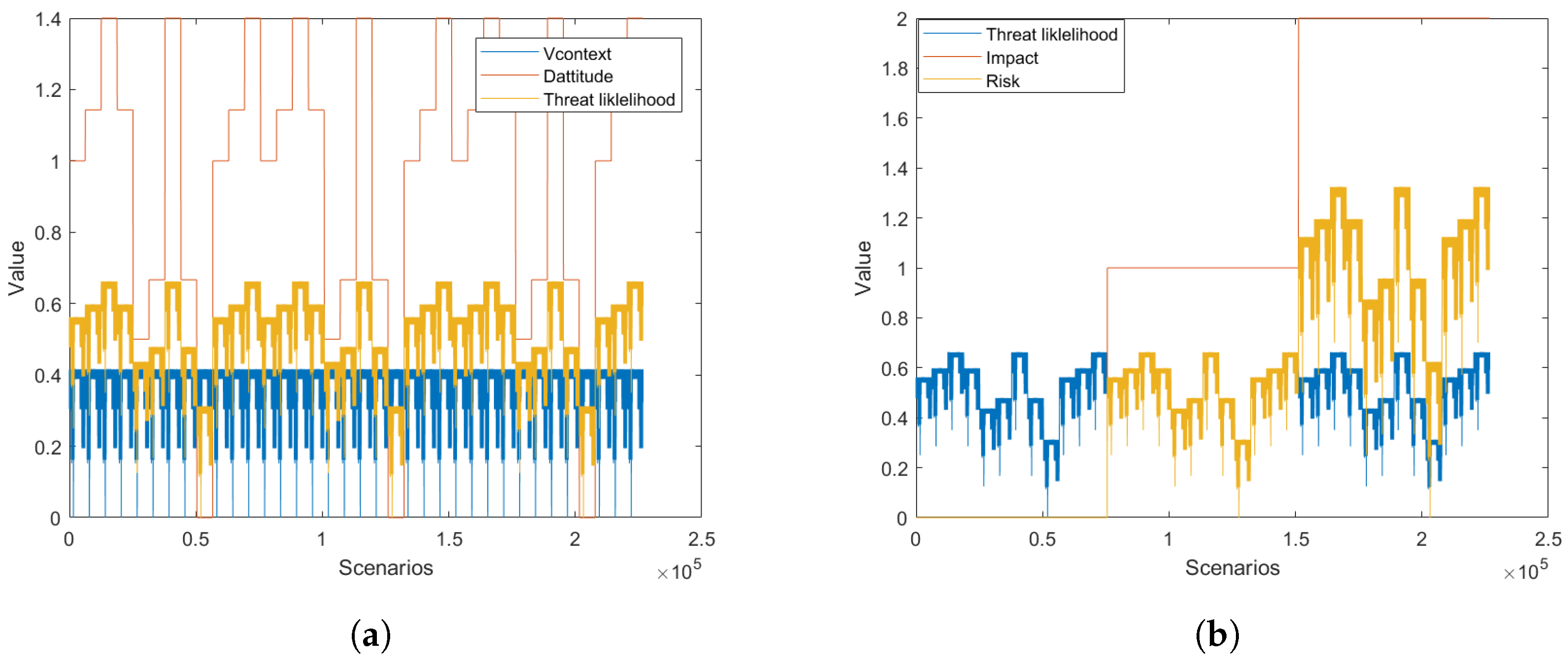
5. Simulation-Based Analysis and Evaluation

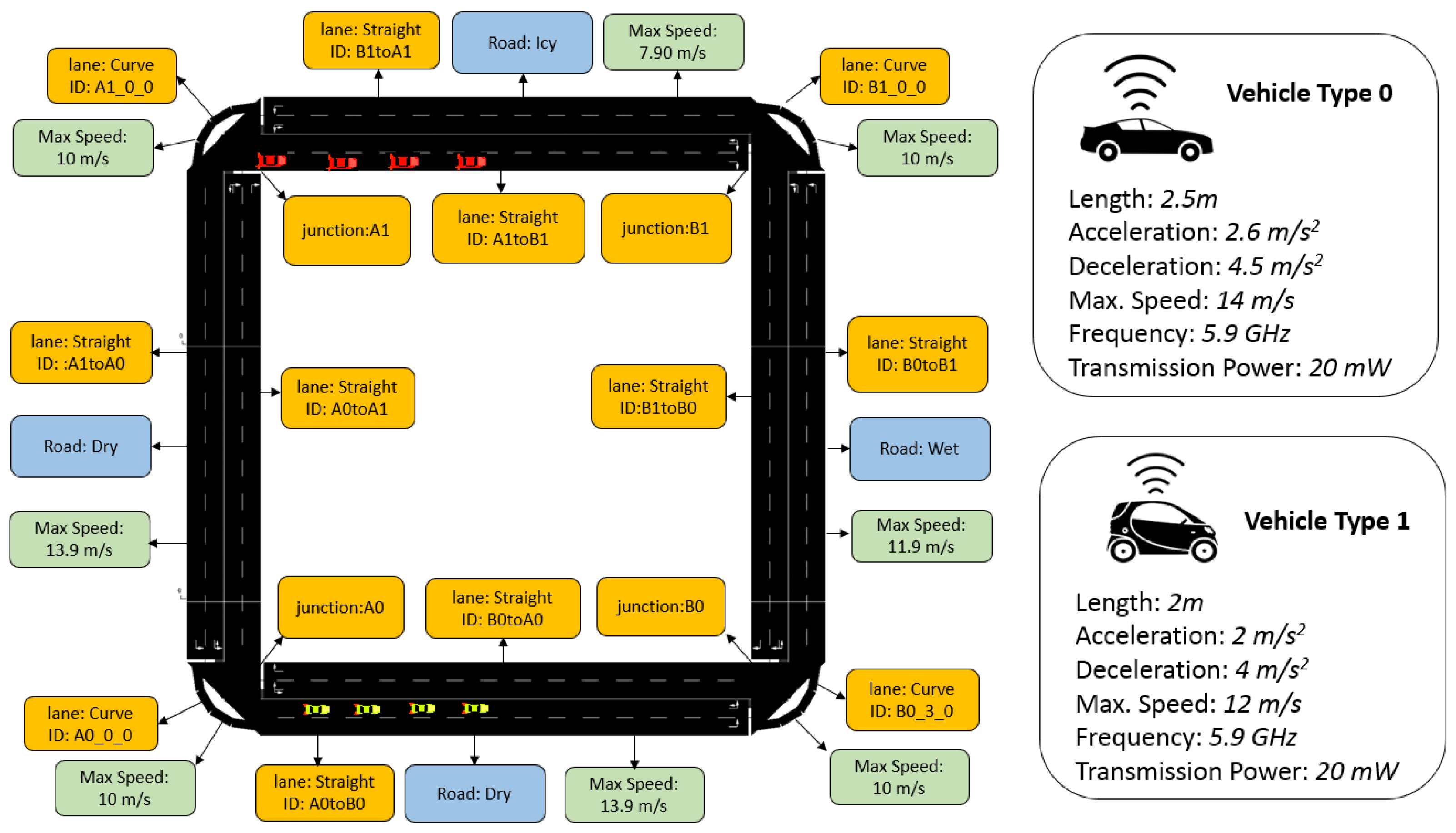
5.1. Simulation Setup and Assumptions

For the proof of concept, we have implemented our proposed extended fuzzy-based risk module in OMNET++ network simulator [15]. For traffic modeling, we used SUMO (simulation of urban mobility) simulator [16]. In order to provide integration between OMNET++ and SUMO network, we used an open source framework called VEINS (vehicles in network simulation) [17]. The basic configurations about roads, lanes, and vehicles are shown in Figure 4.

For the simulation, we have implemented the following three VANET application scenarios.

• Safety-related application scenario: For this scenario, we have implemented an accident notification application. The accident scenario is implemented by setting the speed of the vehicle to zero at a particular time. At the time of the accident, the vehicle will flood the “accident message”. The neighboring vehicles that received this message will change their route and relay this message to other vehicles. The message related to the same event will only be relayed once.
• Traffic efficiency related application scenario: For this scenario, we have implemented the traffic jam notification application. At the time of congestion, the vehicle will flood the “congestion message”. The neighboring vehicles that received this message will slow down and relay this message to other vehicles. Similar to the accident notification application, the message related to the same event will only be relayed once.
• Infotainment related application scenario: This is a simple scenario, in which vehicles share any random infotainment message to other vehicles. On the reception of infotainment message, the behavior of the vehicle and traffic will not be changed.

All above-mentioned three applications are attached to each vehicle in the simulation. Other assumptions and specifications are given below.

• In order to determine the time of the day, we have divided the simulation time into four portions: (1) 0–5 simulation time range is considered as “dawn”, (2) 5 to 25 time range is considered as “day”, (3) 25 to 30 time range is considered as “dusk”, and (4) 30 onwards is considered as “night”.
• Throughout the simulation, we have assumed clear weather.
• Driver Age and Experience are randomly assigned to each vehicle by keeping the following condition intact: Experience should always be less than Age.
• Two types of vehicles are created in the simulation: (1) type 0 and (2) type 1. The length of type 0 vehicles is larger than the type 1 vehicles. Also, the speed of the type 0 is also higher than the type 1 vehicles.
• The following two traffic flows are generated:
  • $A0toB0\to B0toB1\to B1toA1\to A1toA0$,
  • $A1toB1\to B1toB0\to B0toA0\to A0toA1$.
  The first flow comprises of four type 0 vehicles and second flow comprises of four type 1 vehicles.

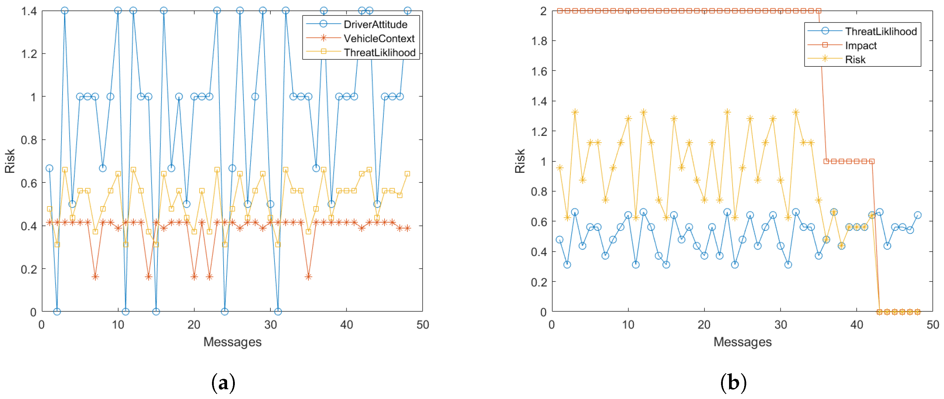
As discussed earlier, each vehicle calculates the risk value on the reception of the message based on the information available locally. For the risk calculation, no interactions (e.g., peer recommendation) with other vehicles will be carried out and there will be no dependency on other vehicles for decision making. Therefore, the proposed scheme is scalable for a large number of vehicles like city scenarios and congested highways. However, for the simplicity and proof-of-concept, we implemented a square-shaped multilane two-way road structure with eight cars as shown in Figure 4. The remaining OMNET++ simulation configuration information is given in

Table 6. OMNET++ configuration.

Parameter	Value
Simulation time	80 s
Number of cars	8
frequency	5.9 GHz
Transmission power	20 mW
Bandwidth	10 MHz
Channel number	3

. At the physical layer, vehicles communicate with each other using IEEE 802.11 protocol. For the application layer communication, we developed a customized application layer packet using VEINS-INET framework, which contains the fields shown in

Table 7. Customized application layer packet format.

$\mathit{Fields}:$	Road Id	Lane Id	Lane Position	App Type	Payload
Datatype:	string	string	double	integer	string
length:	6 bytes	6 bytes	4 bytes	2 bytes	200 bytes

.

5.2. Results

The objective of this simulation was to determine the effect of risk model on travel duration, and communication overhead. For this purpose, we have run the simulation in two setups: (1) Without risk model, and (2) extended fuzzy risk model.

In the first setup, on the reception of the message (accident/congestion/infotainment), the vehicle will take appropriate application-specific action (as discussed earlier in preceding subsection) and then it will be relayed to other vehicles.

In the second setup, on the reception of the message (accident/congestion/infotainment), vehicle first determines the risk value based on the vehicle context, driver attitude and application type. If the risk value is less than the predefined threshold (we assumed 50% of maximum risk value) then application specific action will be taken and relayed to other vehicles. In other case, the message will be discarded.

Figure 5 shows the risk calculation of all the messages received by various vehicles. At four instances the risk value was 1.3237, which is maximum. At six instances, the risk value was zero, which is minimum. At 38 instances, the risk value was between zero and 1.3237. According to Theorem 1, risk value should be between 0 and 1.3237 (inclusively). This figure clearly indicates that for all the messages, the risk value is within the range defined in Theorem 1. It shows that the risk model is implemented correctly in the simulation.

Figure 6 shows the effect of the risk model on communication overhead. It shows that the with risk-based setup, vehicles receives less number of packets and less number of packets were relayed as compared to normal setup. Consequently, less energy will be consumed.

Figure 7 shows the effect of the risk model on travel duration. From travel duration, we mean, how much time a vehicle will take to reach the final destination. Results show that with a risk model, travel duration of vehicles reduces. Consequently, fuel consumption and electricity consumption will also be reduced, which will create a positive impact on the environment and makes the vehicles eco-friendly. In a simple model, fuel consumption and electricity consumption are proportional to the travel duration. If the travel time increase, the fuel consumption and electricity consumption will also increase. With this model, the proposed risk model consumed approximately 23% less fuel or electricity.

Figure 8 shows the average results per vehicle. It shows that incorporating the risk model in VANET applications will help to increase the performance of the network. According to this figure, with risk model, on average vehicles receive 61.6% less packets and 73.91% less packets relayed. Due to these benefits, less energy consumption will be consumed.

For transmitting and receiving packets, a certain level of energy is consumed. In order to determine the energy consumption of the proposed model, we have adopted first order radio model [18], which is widely used for energy consumption analysis in wireless networks. Let us assume that vehicle i has transmitted $n_{tx}$ number of messages and received $n_{rx}$ number of messages. In this case, energy consumption ($Ec$) of vehicle i will be calculated in the following manner.

$$E{c}^i=n_{tx}^i{E}_{tx}(k,d)+n_{rx}^i{E}_{rx}\left(k\right)$$

where $E_{tx}(k,d)$ represents the energy that is required to transmit k bits of packet at distance d, $E_{rx}\left(k\right)$ represents the energy that is required to receive data length of k bits. In our simulation model the length of the packet was 218 bytes ( k = 1744 bits), and d was set as 140 m. Figure 9 shows the energy consumption analysis of the proposed risk model on per vehicle basis. It indicates the risk model can help to reduce energy consumption. On average, the proposed risk model consumes approximately 65% less energy as compared to “without risk” model scenario.

Figure 10 shows the statistical information about the minimum, maximum risk scenarios with respect to the application types that system encountered during the simulation. According to this figure, 12.5% messages leads towards minimum risk, 8.33% messages leads towards maximum risk, and 79.16% messages lead towards risk between minimum and maximum. As shown in Figure 10b, all 12.5% messages which lead towards minimum risk belongs to infotainment application; all 8.33% messages which lead towards maximum risk belongs to safety application; among 79.16% messages which lead towards risk between minimum and maximum, 81.57% belongs to safety application, and remaining 18.42% belongs to traffic efficiency application.

6. Theoretical Analysis and Evaluation

Simulation-based analysis and evaluation is always a constraint with a lot of assumptions and does not cover all possible scenarios. Therefore, we have also conducted theoretical-based analysis and evaluation of the proposed method.

6.1. Dataset Generation

The main problem that we faced during analysis and evaluation is the unavailability of the comprehensive testing dataset which contains all the parameters that are used in the proposed model. In order to overcome this problem, we created our own dataset generator program in the Python language. The code for this program is shown in Figure 11. This program creates a dataset in CSV format. Consequently, it can be easily used with any other tools (e.g., MATLAB, MS Excel, data mining tools, etc.) for further analysis.

With the help of the VANET dataset generator program, we have created a dataset that contains all possible 226,800 different scenarios as shown in

Table 8. VANET dataset.

No.	Application	Age	Experience	Road	Speed	Time	Weather	Lane	Traffic
1	Infotainment	Age <25	Exp <= 10	Dry	Accelerating	Dawn	Clear	Corner	Cars on 1 side
2	Infotainment	Age <25	Exp <= 10	Dry	Accelerating	Dawn	Clear	Corner	Cars on 2 sides
3	Infotainment	Age <25	Exp <= 10	Dry	Accelerating	Dawn	Clear	Corner	Cars on 3 sides
4	Infotainment	Age <25	Exp <= 10	Dry	Accelerating	Dawn	Clear	Corner	Cars on 4 sides
5	Infotainment	Age <25	Exp <= 10	Dry	Accelerating	Dawn	Clear	Corner	No cars
- - snip - -
226,796	Safety	Age >65	Exp >= 30	Wet	Decelerating	Night	Windy	Winding	Cars on 1 side
226,797	Safety	Age >65	Exp >= 30	Wet	Decelerating	Night	Windy	Winding	Cars on 2 sides
226,798	Safety	Age >65	Exp >= 30	Wet	Decelerating	Night	Windy	Winding	Cars on 3 sides
226,799	Safety	Age >65	Exp >= 30	Wet	Decelerating	Night	Windy	Winding	Cars on 4 sides
226,800	Safety	Age >65	Exp >= 30	Wet	Decelerating	Night	Windy	Winding	No cars

. The frequency of each attribute value in a dataset is shown in Figure 12.

6.2. Analysis and Evaluation

For the purpose of analysis and evaluation, we have implemented the proposed fuzzy risk model in the Python language. The source code of this model is also available for the research community along with the dataset. On this dataset, when we applied the proposed model, we get the results shown in Figure 13a,b.

Based on the vehicle context and driver’s attitude, Figure 13a presents the threat likelihood of all 226,800 scenarios. In Section 4, we identified the minimum and maximum values for vehicle context (Proposition A4) and driver’s attitude (Proposition A5). The result shown in this figure proves the correct implementation of the threat likelihood determination.

Figure 13b presents the risk estimation of all the scenarios. It shows that the risk value fluctuates between 0 and 1.3237, which is correct according to the Theorem 1. From further analysis (as depicted in Figure 14), we found that among 226,800 scenarios:

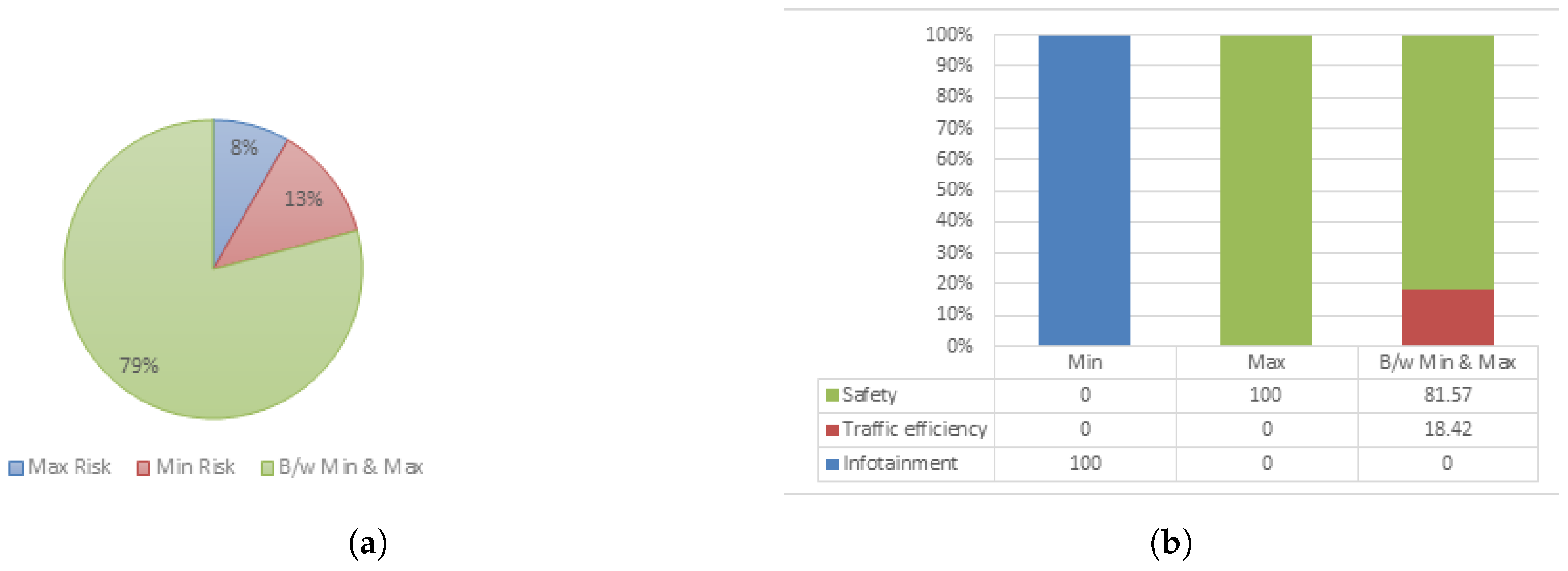
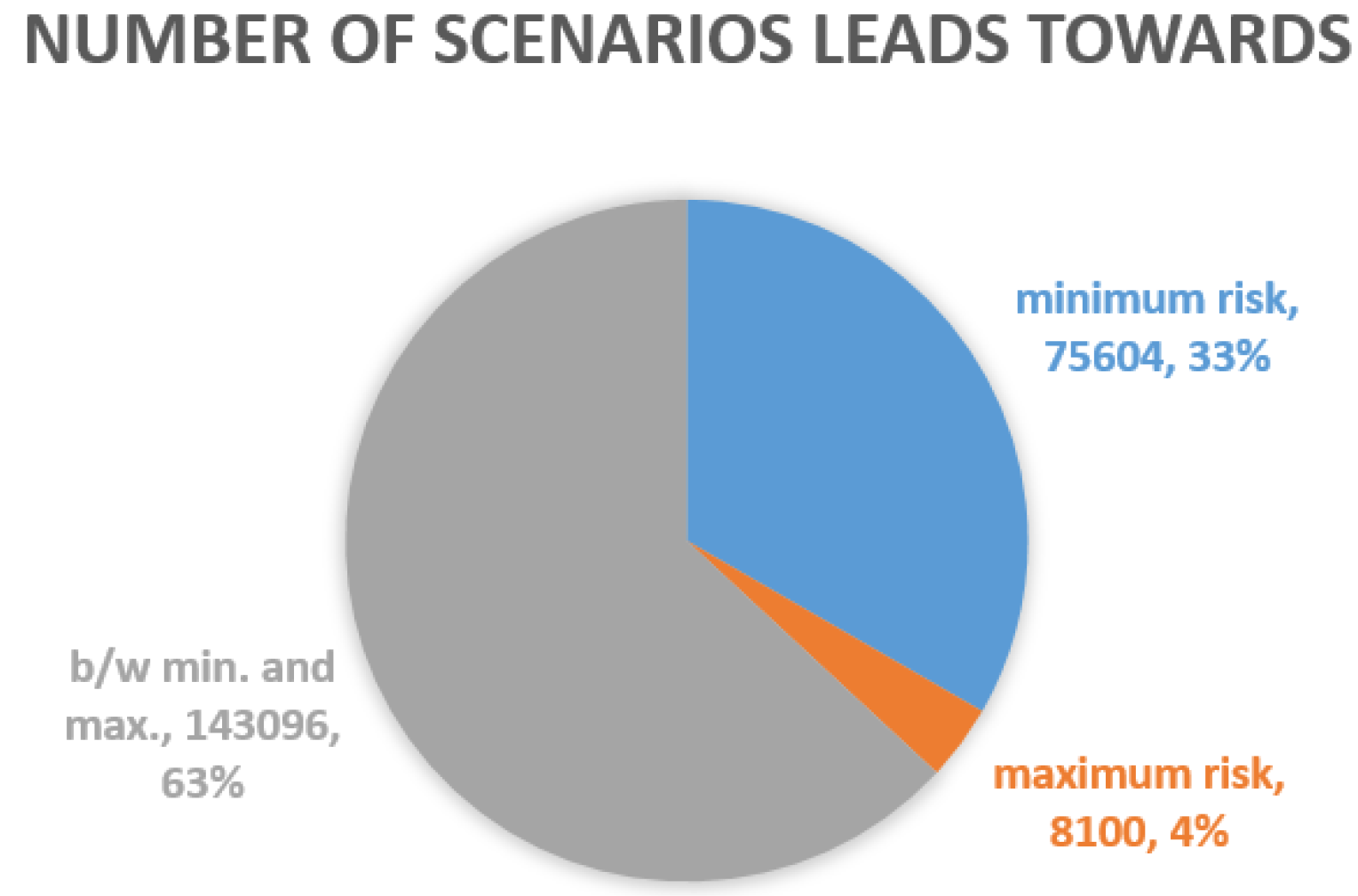
• 75,604 scenarios (33.33%) lead towards minimum risk (zero). This looks high at first glance. However, this is due to the fact that most of those scenarios are assuming infotainment application, which we have categorized as low impact application as discussed in Section 2. As shown in Figure 12, 75,600 scenarios assumed infotainment application. So, all those scenarios lead towards minimum risk. For other scenarios (which are either assuming traffic efficiency related applications or safety-related applications), only four cases exist which lead towards minimum risk.
• 8100 scenarios (3.57%) lead towards maximum risk.
• 143,096 scenarios (63.09%) lead towards risk between minimum and maximum.

6.3. Time and Space Complexity Analysis

Space complexity deals with memory, which holds the data for calculating the risk values and other related operations during the calculations. In this proposed model, character, integer and floating point considered as 1 byte, 2 bytes and 4 bytes, respectively, are used for analyzing the space complexity.

Table 9. Space requirement of existing scheme.

and

Table 10. Space requirement of the proposed scheme.

provide the details of the input data and storage for existing fuzzy risk scheme [12] and the proposed scheme. As shown in Table 9, the space requirement for the existing fuzzy scheme is 266 bytes, whereas the space requirement for the proposed extended fuzzy scheme is 461 bytes (see Table 10), which is just 195 bytes higher than the existing one.

In order to determine the time complexity of the existing fuzzy scheme and proposed scheme, first, we need to determine the number and types (e.g., addition, subtraction, etc.) of arithmetic operations that are needed to calculate risk value. In general, the complexity of addition, and subtraction operation of n digit number is $O\left(n\right)$. Whereas, the complexity of multiplication and division operation is $O\left(n^2\right)$. In the existing and proposed model, finding the minimum and maximum number in an array is also used. For those operations, the complexity in the worst-case scenario is $O\left(n\right)$.

Table 11. Arithmetic operations of existing scheme.

	Addition	Subtraction	Multiplication	Min	Max	Equation No.
Impact	1	5		3	3	2
Risk	1		11		2	3
Total	2	5	11	3	5

2 Addition + 5 subtraction + 3 min + 5 max = $15n$; 11 Multiplication = $11n^2$; Arithmetic Complexity = $11n^2+15n$.

and

Table 12. Arithmetic operations of proposed scheme.

	Addition	Subtraction	Division	Multiplication	Min	Max	Equation No.
Impact	1	5			3	3	2
Risk				11		2	3
Common denominator for $w_1$ to $w_6$	5		6				10–15
$w_1$			2				10
$w_2$			2				11
$w_3$			2				12
$w_4$			2				13
$w_5$			2				14
$w_6$			2				15
${\beta }_1$	1		1				17
${\beta }_2$		1					18
${\alpha }_1$	1		1				19
${\alpha }_2$		1					20
Total	8	7	20	11	3	5

8 Addition + 7 subtraction + 3 min + 5 max = $23n$; 11 Multiplication + 20 Division = $31n^2$; Arithmetic Complexity = $31n^2+23n$.

present the number and types of arithmetic operation for existing fuzzy-based risk scheme and proposed scheme, respectively. According to Table 11, the existing fuzzy risk-based scheme [12] requires 2 addition, 5 subtraction, 11 multiplication, 3 find-minimum, and 5 find-maximum operations. Therefore, the arithmetic complexity for the existing scheme [12] is $11n^2+15n$. Whereas, the proposed extended fuzzy requires 8 addition, 7 subtraction, 20 division, 11 multiplication, 3 find-minimum, and 5 find-maximum operations. Therefore, the arithmetic complexity of the proposed scheme is $31n^2+23n$ (See Table 12). The time complexity for both the schemes is $O\left(n^2\right)$.

7. Related Work and Qualitative Comparison

7.1. Related Work

Chen et al. [8] have proposed probabilistic decision-making framework for rear-end collision avoidance system. Based on a prior probabilistic knowledge and Bayesian network approach, this framework estimates collision risk. This framework classifies risk into two levels: High and low. In case of low risk, the framework will generate audio/video alert. Whereas, in other case, “an automatic braking or steering action will be carried out to force the vehicle to brake or make a lane change”. This framework is limited to single safety application scenario.

Sun et al. [9] have proposed truth-aware decision framework suitable for V2V communications. In their framework, authors have incorporated Bayes rule and Dempster Shafer Theory (DST) for estimating and updating the belief/truthfulness of the message. They also incorporated driver’s preferences (e.g., safety is more important than efficiency or vice versa) in the decision making process. This framework is limited to single hop forwarding and belief combination.

Vijey and Shaikh [10] have proposed a probability distribution based risk estimation model for VANETs. In this model, risk is based on threat likelihood and impact. The threat likelihood is derived based on six different vehicle contextual parameters and impact is derived based on the gap between two vehicles. If the derived risk is above the pre-defined threshold then vehicles will take risk-mitigating decisions. If it is below the threshold then vehicles can increase the speed or move into the fast lane.This framework is limited to single safety application scenario.

Fitzgerald and Landfeldt [11] have proposed risk mitigation techniques for the purpose of maximizing road network throughput and lowered accident rate. The proposed risk model incorporates various driver, environmental and vehicle factors. The individual value of each factor is averaged together to estimate risk value. However, the mechanism for risk value derivation for each factor individually is not discussed in the paper.

McCall and Trivedi [19] addressed issues related to common braking behavior and predicted driver behavioral information through the proposed framework. Datasets of natural driving behaviors are used as a methodology for analyzing all behavioral information. The proposed framework depends on the Bayesian network used for assessing the criticality of driving situations and uses sparse Bayesian learning for estimating probability on different datasets. While it is used for safety applications, it could also be used to improve traffic efficiency.

Glaser et al. [20] proposed an approach which allows drivers to determine an optimal trajectory during the driving. In this approach, the trajectory planning algorithm is employed with two steps which are maneuver and trajectory modules. While maneuver keeps the optimal trajectory every 10 ms, this approach supports to improve the several performances such as risk, speed, etc. This approach supports traffic safety and efficiency applications.

Noh and An [21] conducted research on risk assessment for automatic lane change maneuvers using a risk assessment algorithm. In this algorithm, Bayesian networks are considered with two complementary risk metrics which are time-to-collision and minimum safety margin. To evaluate the risk level, probabilistic reasoning based on Bayesian networks is used in the experiment. This research supports to improve the traffic safety application.

Chen et al. [22] focused on improving V2V communication, fast response and decision making without sacrificing quality and preventing fake information. To improve these problems, authors have proposed a partially observable markov decision process (POMDP) based approach. When malicious vehicles change their behavior, the Bayesian reinforcement learning algorithm is used with POMDP to observe the behavior. While the authors focused on securing V2V communication, infotainment application is indirectly considered.

Schneider et al. [23] have introduced a generic method for probabilistic identification of driving situations and maneuvers considered with Bayesian network and fuzzy features. A measure of the probabilistic situation and maneuver detection provides the quality for interpreting information by a reliable detection. The inaccuracies of the sensor measurements also affect quality. In this research, traffic safety issues are considered an application.

According to Fitzgerald and Landfeldt [24], a modification to the risk mitigation system is introduced as a proposed method. In this modification, the algorithm (weighted average of risk estimation) allows vehicles to exchange risk information and modify their estimated risk from the inputs received from the vehicles. Jacobi with local Gauss-Seidel method supports to converge for finding risk. This mitigation system supports traffic efficiency application through the risk calculation.

Fitzgerald and Landfeldt [25] have extended the model from risk mitigation and management system described in [15]. In this extended model, authors developed a risk-aware link choice algorithm to estimate the risk in each link. This algorithm not only deals with congestion problems but also calculates the varied risk differences. This extended model supports the traffic efficiency application.

Gindele et al. [26] addressed issues related to decision making and motion planning when a proposed probabilistic model uses a filter. It allows vehicles to estimate the current position, behavior and predictable trajectory. In this model, dynamic Bayesian network plays an important role in calculating the inference efficiently with the rao-blackwellized method which reduces the complexity. The further machine learning method is considered to improve tracking. This proposed method provides traffic safety in the application.

According to Niehaus and Stengel [27], rule-based systems are investigated for autonomous vehicles to plan a safe trajectory. Here, the authors proposed a probabilistic framework for automated decision making and improving the traffic safety through intelligent guidance for headway and lane control (IGHLC) systems. Framework and IGHLC can be used in a traffic safety application.

As Noh et al. [28] mentioned, the high-level data fusion based probabilistic situation assessment method is considered as a proposed approach to eliminate the threat level of the lanes. This method consists of two parts which provide the current traffic situation and recommendation to take the precautions with driving behaviors. This assessment method supports a traffic safety application.

Naranjo et al. [29] proposed an approach which is for autonomous vehicles equipped with path-tracking and lane-change capabilities. In this approach, fuzzy controllers and high-precision global positioning system allow autonomous vehicles to overtake the other vehicle. While this approach supports autonomous vehicles, traffic safety application is focused on more.

Table 13. Summary of related work.

Reference	Methodology	Application Domain
[8]	Probabilistic model + Bayesian network	Supports single safety application scenario
[9]	Bayes rules + Dempster Shafer theory	Supports multiple application scenarios
[10]	Probabilistic model	Supports single safety application scenario
[11]	Simple average	Supports multiple application scenarios
[19]	Bayesian framework +probabilistic model	Supports multiple application scenarios
[20]	Trajectory-planning algorithm	Supports single traffic safety application
[21]	Probabilistic reasoning based on Bayesian networks	Supports single traffic safety application
[22]	Partially observable markov decision process (POMDP) with Bayesian theory	Supports multiple application scenarios
[23]	Bayesian network and fuzzy features	Support for multiple application scenarios
[24]	Risk mitigation with an algorithm using a weighted average of risk estimates	Supports single traffic efficiency application
[25]	Risk-aware link choice algorithm	Supports single traffic efficiency application
[26]	Probabilistic model and Bayesian network	Supports single traffic safety application
[27]	Probabilistic framework with stochastic function	Supports single traffic safety application
[28]	Probabilistic situation assessment method	Supports single traffic safety application
[29]	Fuzzy controllers and high-precision global positioning system	Supports single safety application scenario

summarized the above mentioned schemes.

7.2. Qualitative Comparison

The parameters used in risk estimation can broadly be classified into the following four factors.

• Environmental factors: Road, lane, weather, time, traffic, etc.
• Vehicle factors: Speed, model, length, etc.
• Driver factors: Age, experience, gender, emotions, etc.
• Application specific factors: Type, sensitivity level, event messages, etc.

Based on these factors, the classification of existing schemes is shown in

Table 14. Classification of existing schemes.

	Factors
	Environmental	Vehicle	Driver	Application
Proposed Model	×	×	×	×
[8]	×	×
[9]	×	×
[10]	×	×
[11]	×	×	×
[19]	×	×
[20]	×	×
[21]	×	×
[22]	×			×
[23]	×
[24]	×	×	×
[25]	×	×	×
[26]		×
[27]	×	×
[28]	×	×
[29]	×

. From this table, we noticed that most of the existing schemes evaluated risk based on environmental and vehicle related factors. Only a few works incorporated driver and application specific factors. This table also shows that only our proposed model covers all four factors, which increases its reliability and completeness.

As shown in Table 14, most of the schemes considered environmental factors. However, not all schemes considered the same environmental factors as shown in

Table 15. Environmental factors comparison.

	Road	Lane	Weather	Time	Traffic
Proposed Model	×	×	×	×	×
[8]	×		×	×	×
[9]	×		×
[10]	×	×	×	×	×
[11]		×			×
[19]					×
[20]		×			×
[21]		×			×
[22]					×
[23]		×
[24]	×
[25]	×	×
[26]
[27]		×			×
[28]		×			×
[29]		×			×

. The majority of the schemes incorporated traffic and lane related conditions. Very few schemes incorporated road (dry, wet, icy, etc.), time (night, day, etc.) and weather (rainy, snowy, etc.) conditions. This table also indicates that the proposed scheme incorporated most of the environmental factors.

Table 16. Vehicle and driver factors comparison.

	Vehicle Factors			Driver Factors
	Speed	Type	Length	Age	Experience	Gender
Proposed Model	×			×	×
[8]	×
[9]	×
[10]	×	×	×
[11]	×	×		×		×
[19]	×
[20]	×
[21]	×
[22]
[23]
[24]	×	×		Not clearly specified
[25]	×			Not clearly specified
[26]	×
[27]	×
[28]	×
[29]

presents the comparison from the perspective of three vehicle factors (speed, type and length) and three driver factors (age, experience and gender). This table shows that most of the schemes incorporate speed of the vehicle in measuring risk. Very few schemes incorporate driver factors.

8. Future Research Issues and Challenges

After we use all parameters mentioned in the paper, we have proved that the risk-based decision method allows transport service providers to minimize the risks in the vehicular networks. Despite these parameters, when we use the lane spaces with an intelligent approach, we can minimize not only the risks but also the accidents. Here, intelligent approach means that using intelligent decision making [30] according to the situation will be better to improve the future autonomous vehicles (driverless vehicles). Lane spaces and gaps between the vehicles should be maintained with the time which is one of the key elements for making an intelligent decision.

When we use intelligent approaches, we can reduce the risk values which will improve the transportation facilities such as better communication services. Deciding speed of vehicles depends on many factors such as time management between the vehicles, size of the vehicles, lane spaces, etc. When we increase the speed of the vehicles intelligently, expected risk values may be better because the number of vehicles per km is less.

9. Conclusions and Future Work

Incorporating risk in a decision-making processes increases the reliability of the system. In vehicular networks, intelligent decision making is very critical for achieving traffic efficiency and road safety. In practice, the vehicular network may contain faulty or malicious vehicles, who may forward or share fake and inaccurate information. Consequently, this may cause undesirable things, such as automobile fatalities and traffic congestion. Therefore, it is highly desirable to evaluate risk before a vehicle takes any decision based on the received information.

For VANETs, various risk-based decision systems exist in the literature. Our proposed fuzzy risk-based decision model is one of them. In order to make this model more robust, and reliable, we have proposed many improvements in this paper. A dataset has also been presented for theoretical analysis and evaluation. For cross-validation of theoretical results, we have also presented theorems and proofs. Additionally, we have also presented a simulation-based analysis and evaluation of the proposed scheme. In general, results show that the proposed methodologies will play an important role in increasing traffic efficiency and traveler comfort to a certain degree.

In the future, we would like to perform more realistic simulations by incorporating RSU, V2I communications, and real world road networks.

References

1. Ahmad, F.; Franqueira, V.N.; Adnane, A. TEAM: A trust evaluation and management framework in context-enabled vehicular ad-hoc networks. IEEE Access 2018, 6, 28643–28660. [Google Scholar] [CrossRef]
2. Shaikh, R.A.; Alzahrani, A.S. Intrusion-aware trust model for vehicular ad hoc networks. Secur. Commun. Netw. 2014, 7, 1652–1669. [Google Scholar] [CrossRef]
3. Kong, H.; Kim, T.; Hong, M. A Security Risk Assessment Framework for Smart Car. In Proceedings of the 10th International Conference on Innovative Mobile and Internet Services in Ubiquitous Computing (IMIS), Fukoaka, Japan, 6–8 July 2016; pp. 102–108. [Google Scholar] [CrossRef]
4. Hill, C.J.; Garrett, J.K. AASHTO Connected Vehicle Infrastructure Deployment Analysis, FHWA-JPO-11-090; Technical Report; American Association of State Highway and Transportation Officials AASHTO: Washington, DC, USA, 2011. [Google Scholar]
5. Shaikh, R.A.; Alzahrani, A.S. Trust Management Method for Vehicular Ad Hoc Networks. In Quality, Reliability, Security and Robustness in Heterogeneous Networks; Singh, K., Awasthi, A.K., Eds.; Springer: Berlin/Heidelberg, Germany, 2013; pp. 801–815. [Google Scholar]
6. Beltz, B. Car Accidents Statistics. Available online: https://safer-america.com/car-accident-statistics/ (accessed on 6 March 2019).
7. Zhao, H.; Mao, T.; Yu, H.; Zhang, M.K.; Zhu, H. A Driving Risk Prediction Algorithm Based on PCA -BP Neural Network in Vehicular Communication. In Proceedings of the 10th International Conference on Intelligent Human-Machine Systems and Cybernetics (IHMSC), Hangzhou, China, 25–26 August 2018; pp. 164–169. [Google Scholar] [CrossRef]
8. Chen, C.; Liu, X.; Chen, H.; Li, M.; Zhao, L. A Rear-End Collision Risk Evaluation and Control Scheme Using a Bayesian Network Model. IEEE Trans. Intell. Transp. Syst. 2019, 20, 264–284. [Google Scholar] [CrossRef]
9. Sun, M.; Li, M.; Gerdes, R. Truth-aware Optimal Decision-making Framework with Driver Preferences for V2V Communications. In Proceedings of the IEEE Conference on Communications and Network Security (CNS), Beijing, China, 30 May–1 June 2018; pp. 1–9. [Google Scholar] [CrossRef]
10. Thayananthan, V.; Shaikh, R.A. Contextual Risk-based Decision Modeling for Vehicular Networks. Int. J. Adv. Comput. Sci. Appl. 2016, 8, 1–9. [Google Scholar] [CrossRef]
11. Fitzgerald, E.; Landfeldt, B. Increasing road traffic throughput through dynamic traffic accident risk mitigation. J. Transp. Technol. 2015, 5, 223–239. [Google Scholar] [CrossRef]
12. Shaikh, R.A. Fuzzy Risk-based Decision Method for Vehicular Ad Hoc Networks. Int. J. Adv. Comput. Sci. Appl. 2016, 7, 54–62. [Google Scholar] [CrossRef]
13. Transportation Research Center for Livable Communities. Available online: https://wmich.edu/transportationcenter/trclc-14-8 (accessed on 15 May 2019).
14. Stoneburner, G.; Goguen, A.Y.; Feringa, A. Risk Management Guide for Information Technology Systems, Sp 800-30; Technical Report; National Institute of Standards & Technology: Gaithersburg, MA, USA, 2002. [Google Scholar]
15. OMNET Simulator. Available online: https://www.omnetpp.org/ (accessed on 19 February 2019).
16. SUMO (Simulation of Urban Mobility) Simulator. Available online: http://sumo.sourceforge.net/ (accessed on 19 February 2019).
17. VEINS Framework. Available online: http://veins.car2x.org/ (accessed on 19 February 2019).
18. Heinzelman, W.R.; Chandrakasan, A.; Balakrishnan, H. Energy-efficient communication protocol for wireless microsensor networks. In Proceedings of the 33rd Annual Hawaii International Conference on System Sciences, Maui, HI, USA, 7 January 2000; p. 10. [Google Scholar] [CrossRef]
19. McCall, J.C.; Trivedi, M.M. Driver Behavior and Situation Aware Brake Assistance for Intelligent Vehicles. Proc. IEEE 2007, 95, 374–387. [Google Scholar] [CrossRef]
20. Glaser, S.; Vanholme, B.; Mammar, S.; Gruyer, D.; Nouvelière, L. Maneuver-based Trajectory Planning for Highly Autonomous Vehicles on Real Road with Traffic and Driver Interaction. IEEE Trans. Intell. Transp. Syst. 2010, 11, 589–606. [Google Scholar] [CrossRef]
21. Noh, S.; An, K. Risk assessment for automatic lane change maneuvers on highways. In Proceedings of the IEEE International Conference on Robotics and Automation (ICRA), Singapore, 29 May–3 June 2017; pp. 247–254. [Google Scholar] [CrossRef]
22. Chen, S.; Irissappane, A.A.; Zhang, J. POMDP-Based Decision Making for Fast Event Handling in VANETs. In Proceedings of the Thirty-Second AAAI Conference on Artificial Intelligence, New Orleans, LA, USA, 2–7 February 2018; pp. 4646–4653. [Google Scholar]
23. Schneider, J.; Wilde, A.; Naab, K. Probabilistic approach for modeling and identifying driving situations. In Proceedings of the 2008 IEEE Intelligent Vehicles Symposium, Eindhoven, The Netherlands, 4–6 June 2008; pp. 343–348. [Google Scholar] [CrossRef]
24. Fitzgerald, E.; Landfeldt, B. A system for coupled road traffic utility maximisation and risk management using VANET. In Proceedings of the 2012 15th International IEEE Conference on Intelligent Transportation Systems, Anchorage, AK, USA, 16–19 September 2012; pp. 1880–1887. [Google Scholar] [CrossRef]
25. Fitzgerald, E.; Landfeldt, B. On road network utility based on risk-aware link choice. In Proceedings of the 16th International IEEE Conference on Intelligent Transportation Systems (ITSC 2013), The Hague, The Netherlands, 6–9 October 2013; pp. 991–997. [Google Scholar] [CrossRef]
26. Gindele, T.; Brechtel, S.; Dillmann, R. A probabilistic model for estimating driver behaviors and vehicle trajectories in traffic environments. In Proceedings of the 13th International IEEE Conference on Intelligent Transportation Systems, Funchal, Portugal, 19–22 September 2010; pp. 1625–1631. [Google Scholar] [CrossRef]
27. Niehaus, A.; Stengel, R.F. Probability-based decision making for automated highway driving. IEEE Trans. Veh. Technol. 1994, 43, 626–634. [Google Scholar] [CrossRef] [Green Version]
28. Noh, S.; An, K.; Han, W. High-Level Data Fusion Based Probabilistic Situation Assessment for Highly Automated Driving. In Proceedings of the 2015 IEEE 18th International Conference on Intelligent Transportation Systems, Las Palmas, Spain, 15–18 September 2015; pp. 1587–1594. [Google Scholar] [CrossRef]
29. Naranjo, J.E.; Gonzalez, C.; Garcia, R.; de Pedro, T. Lane-Change Fuzzy Control in Autonomous Vehicles for the Overtaking Maneuver. IEEE Trans. Intell. Transp. Syst. 2008, 9, 438–450. [Google Scholar] [CrossRef] [Green Version]
30. Albeshri, A.; Thayananthan, V. Analytical Techniques for Decision Making on Information Security for Big Data Breaches. Int. J. Inf. Technol. Decis. Mak. 2018, 17, 527–545. [Google Scholar] [CrossRef] [Green Version]
Figure 1. Multilane traffic scenarios. (a) Multi-lane one way road scenario; (b) Multi-lane two way road scenario.
Electronics 08 00627 g001
Figure 2. Risk scenarios for age and experience.
Electronics 08 00627 g002
Figure 3. Adaptive weights values of α 1 and α 2 .
Electronics 08 00627 g003
Figure 4. Road map and specifications.
Electronics 08 00627 g004
Figure 5. Simulation-based Risk analysis. (a) Threat likelihood for each message; (b) Risk values for each message.
Electronics 08 00627 g005
0.450.45
(a) b(b) b
Figure 6. Simulation-based communication overhead analysis. (a) Number of packets relayed; (b) Number of packets received.
Electronics 08 00627 g006
Figure 7. Travel time of each vehicle during simulation.
Electronics 08 00627 g007
Figure 8. Average simulation-based results per vehicle.
Electronics 08 00627 g008
Figure 9. Energy analysis per vehicle.
Electronics 08 00627 g009
Figure 10. Statistical analysis of simulation-based results. (a) Overall risk level distribution; (b) Application specific risk distribution.
Electronics 08 00627 g010
Figure 11. Python code for VANET DataSet generator.
Electronics 08 00627 g011
Figure 12. Frequency of each attribute in the DataSet.
Electronics 08 00627 g012
Figure 13. Theoretical risk analysis. (a) Threat likelihood for each scenario; (b) Risk estimation for each scenario.
Electronics 08 00627 g013
Figure 14. Classification of risk scenarios in dataset.
Electronics 08 00627 g014