Wavelet-Integrated Deep Networks for Single Image Super-Resolution

Abstract

We propose a scale-invariant deep neural network model based on wavelets for single image super-resolution (SISR). The wavelet approximation images and their corresponding wavelet sub-bands across all predefined scale factors are combined to form a big training data set. Then, mappings are determined between the wavelet sub-band images and their corresponding approximation images. Finally, the gradient clipping process is used to boost the training speed of the algorithm. Furthermore, stationary wavelet transform (SWT) is used instead of a discrete wavelet transform (DWT), due to its up-scaling property. In this way, we can preserve more information about the images. In the proposed model, the high-resolution image is recovered with detailed features, due to redundancy (across the scale) property of wavelets. Experimental results show that the proposed model outperforms state-of-the algorithms in terms of peak signal-to-noise ratio (PSNR) and structural similarity index measure (SSIM).

1. Introduction

Single image super-resolution (SISR) is generally posed as an inverse problem in the image processing field. Here, the task is to recover the original high-resolution (HR) image from a single observation of the low-resolution (LR) image. This method is generally used in applications where the HR images are of importance, such as brain image enhancement [1], biometric image enhancement [2], face image enhancement [3], and standard-definition television (SDTV) and high definition television (HDTV) applications [4]. The problem of SISR is considered a highly ill-posed problem, because the number of unknown variables from an HR image is much higher compared to the known ones from an LR image.

In the literature for SISR, a number of algorithms have been proposed for the solution of this problem. They can be categorized as including an interpolation algorithm [5], edge-based algorithm [6], and example-based algorithms [7,8,9]. The interpolation and edge-based algorithms provide reasonable results. However; their performance severely degrades with the increase in an up-scale factor. Recently, the neural network-based algorithms have captured the eye of researchers for the task of SISR [10,11,12]. The main reasons can be the huge capacity of the neural network models and end-to-end learning, which helps researchers to get rid of the features used in the previous approaches.

However, the algorithms proposed so far are unable to achieve better performance for higher scale-ups. The proposed algorithm is a wavelet domain-based algorithm inspired by the category of the SISR algorithms in the wavelet domain [13,14,15,16,17]. Most of these algorithms give state-of-the-art results. However, their computational cost is quite high. With the advances in deep-learning algorithms, the task of computational cost is much reduced with acceptable quality.

Authors in [16], proposed a wavelet domain-based deep learning algorithm with three layers, inspired by the super-resolution convolution neural network (SRCNN) [8] and using a discrete wavelet transform (DWT), and achieved good results. However, the authors fail to capture the full potential of deep learning and wavelets. In this paper, we propose a wavelet domain-based algorithm for the task of SISR. We incorporate the merits of neural network-based end-to-end learning and large model capacity [18], along with the properties of the wavelet domain, such as sparsity, redundancy, and directionality [19,20]. We propose the use of stationary wavelet transform (SWT) for the wavelet domain analysis and synthesis, owing to its up-sampling property over the DWT down-sampling. By doing so, we want to preserve more contextual information about the images. Moreover, we propose the use of deep neural network architecture in the wavelet domain.

More specifically, we train our network between the wavelet approximation images and their corresponding wavelet sub-band images for the task of SISR. By experimental analysis, we show that the proposed deep-network architecture in the wavelet domain can improve performance for the task of SISR with a reasonable computational cost. The proposed algorithm is compared with recent and state-of-the-art algorithms in terms of peak signal-to-noise ratio (PSNR) and structural similarity index measure (SSIM) over the publicly available data sets of “Set5”, “Set14”, “BSD100”, and “Urban100” for different scale factors.

The rest of the paper is organized as follow. Section 2 describes the details about related work. Section 3 describes the details about the proposed method. Section 4 gives an experimental discussion about the properties of the proposed model. Section 5 given the discussion about the experiments and comparative analysis, and Section 6 concludes the paper.

2. Related Work

The proposed algorithm falls into the category of wavelet domain-based SISR algorithms. Authors in [13] proposed a dictionary learning-based algorithm in the wavelet domain. The proposed algorithm learns compact dictionaries for the task of SISR. A similar approach utilizing dictionary learning is proposed in [14], utilizing the DWT. Authors in [15] proposed coupled dictionary learning in the wavelet domain, utilizing the properties of the wavelets with the coupled dictionary learning approach. Another algorithm that utilizes the dual-tree complex wavelet transform (DT-CWT), along with the coupled dictionary and mapping learning for the task of SISR, is proposed in [17]. Authors in [16] utilize the convolution neural networks in the wavelet domain using the DWT, and propose an efficient model for the task of SISR.

In the wavelet-based SISR approaches [13,14,15,16], the main point to note is that they assume the LR image as the level-1 approximation image of the wavelet decomposition. Here, to recover the HR image, the task is to estimate the wavelet sub-band images representing this approximation image, and finally doing one-level inverse wavelet transform. By doing so, authors induce sparsity and directionality along with compactness in the algorithms, which helps boosts the performance of the algorithms as well as improve their convergence speed.

Dong et al. [8] exploited a fully convolution neural network (CNN). In this method, they proposed a three-layer network where complex non-linear mappings are learned between the HR and LR image patches. Authors in [18] propose deep network architecture for the task of SISR. Instead of using the HR and LR images for training, they utilized the residual images, and to boost the convergence of their algorithm, they utilized adjustable gradient clipping. Authors in [8] further propose the sped-up version of the super-resolution convolution neural network (SRCNN) algorithm, called a fast super-resolution convolution neural network (FSRCNN) [21] algorithm. They achieve this by learning the mappings between the HR and LR images without interpolations, along with shrinking the mappings in the feature learning step. Also, the authors decrease the size of filters and increase the number of layers. Authors in [22] propose a deep residual learning network with batch normalizations for the task of SISR, called a deep-network convolution neural network (DnCNN) algorithm. Authors in [23] propose an information distillation network (IDN) algorithm for the task of SISR. They propose a compact network that utilizes the mixing of features and compression to infer more information for the SISR problem. Authors in [24] propose a super-resolution with multiple degradations (SRMD) algorithm for the problem of SISR. They propose the deep network model for SR, utilizing the degradation maps achieved using the dimensionality reduction of principle component analysis (PCA) and then stretching. By doing so, they learned a single network model for multiple scale-ups.

There are several applications related to single image super-resolution, pattern recognition, neural networks, etc., which can be applied in our human’s daily life as well as in human biology. In [25,26], authors have applied different algorithms of neural networks that focus on magnetic resonance imaging (MRI), while in [27,28,29], authors have applied different algorithms of neural networks that focus on human motion and character control. Likewise, our proposed work can be applied in different applications: brain image enhancement, face image enhancement, and SDTV and HDTV applications. The proposed model can be effectively extended to other image processing and pattern recognition applications.

3. Proposed Method

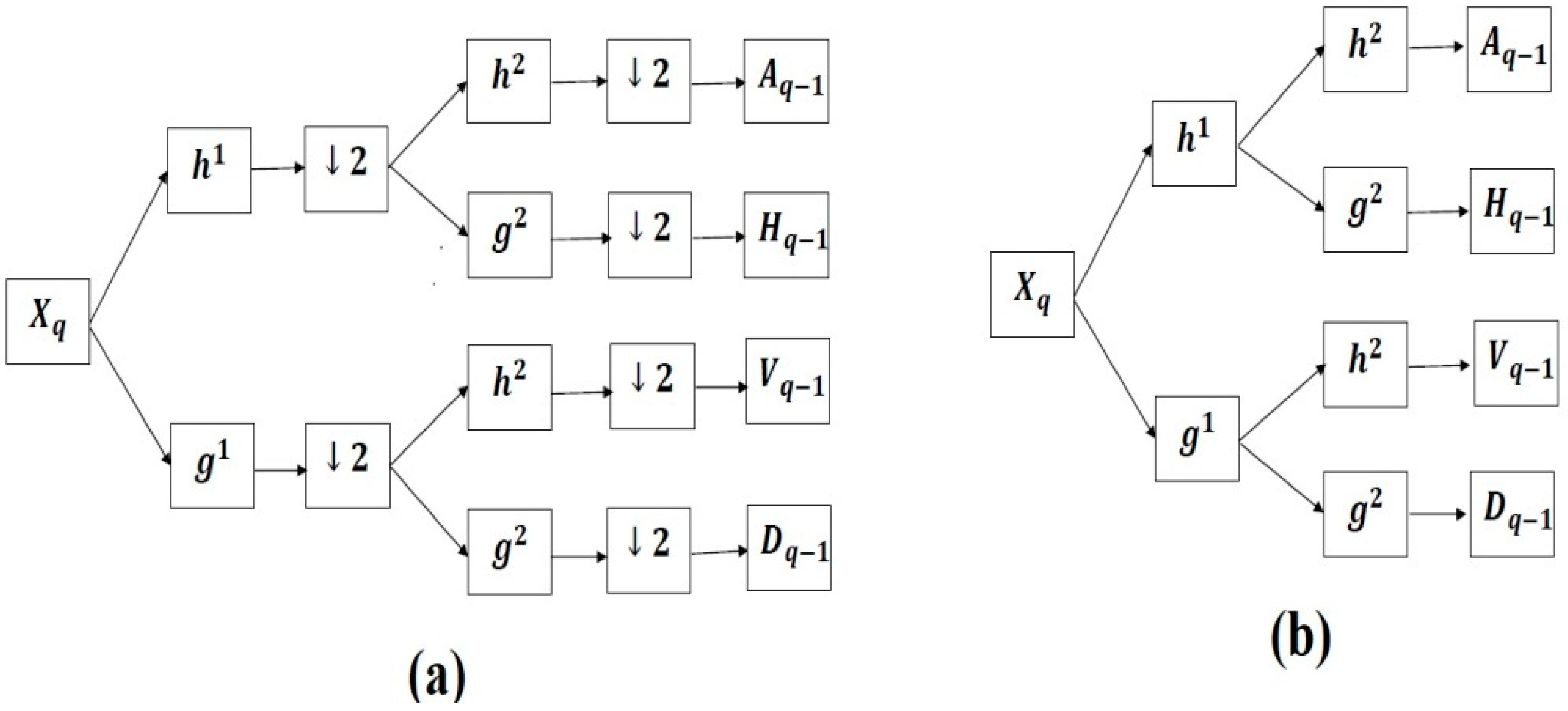
We propose a deep neural network model based on wavelets and gradient clipping for SISR. The wavelet domain-based algorithm was chosen because of the unique properties of the wavelets: they exploit multi-scale modeling, and wavelet sub-bands are significantly sparse. Moreover, instead of DWT, we propose the use of SWT. DWT is a down-sampling process and SWT is an up-sampling process, so the size of the wavelet approximation and sub-bands remains the same, while preserving all the essential properties of the wavelets.

The DWT and SWT decompositions are shown in Figure 1. Further, the wavelet domain-based algorithms consider the LR image as the wavelet approximation image of the corresponding HR image. The task is to estimate its detailed coefficients, as done in [30,31,32,33].

$${\mathrm{A}}_{\mathrm{q}}\left(\mathrm{m},\mathrm{n}\right)={\displaystyle \sum }_{\mathrm{l}=\mathrm{j}}^{\mathrm{M}}{\displaystyle \sum }_{\mathrm{j}=1}^{\mathrm{N}}{\mathrm{h}}_{\mathrm{l}=1}^1{\mathrm{h}}_{\mathrm{j}=1}^2{\mathrm{A}}_{\mathrm{q}}\left(\mathrm{l},\mathrm{j}\right),$$

(1)

$${\mathrm{H}}_{\mathrm{q}}\left(\mathrm{m},\mathrm{n}\right)={\displaystyle \sum }_{\mathrm{l}=\mathrm{j}}^{\mathrm{M}}{\displaystyle \sum }_{\mathrm{j}=1}^{\mathrm{N}}{\mathrm{h}}_{\mathrm{l}=1}^1{\mathrm{h}}_{\mathrm{j}=1}^2{\mathrm{A}}_{\mathrm{q}}\left(\mathrm{l},\mathrm{j}\right),$$

(2)

$${\mathrm{V}}_{\mathrm{q}}\left(\mathrm{m},\mathrm{n}\right)={\displaystyle \sum }_{\mathrm{l}=\mathrm{j}}^{\mathrm{M}}{\displaystyle \sum }_{\mathrm{j}=1}^{\mathrm{N}}{\mathrm{g}}_{\mathrm{l}=1}^1{\mathrm{h}}_{\mathrm{j}=1}^2{\mathrm{A}}_{\mathrm{q}}\left(\mathrm{l},\mathrm{j}\right),$$

(3)

$${\mathrm{D}}_{\mathrm{q}}\left(\mathrm{m},\mathrm{n}\right)={\displaystyle \sum }_{\mathrm{l}=\mathrm{j}}^{\mathrm{M}}{\displaystyle \sum }_{\mathrm{j}=1}^{\mathrm{N}}{\mathrm{g}}_{\mathrm{l}=1}^1{\mathrm{g}}_{\mathrm{j}=1}^2{\mathrm{A}}_{\mathrm{q}}\left(\mathrm{l},\mathrm{j}\right),$$

(4)

where ${\mathrm{h}}_{\mathrm{m}}^1,{\mathrm{h}}_{\mathrm{n}}^2,{\mathrm{g}}_{\mathrm{m}}^1,{\mathrm{and}\mathrm{g}}_{\mathrm{n}}^2$ are the wavelet analysis filters for the SWT. ${\mathrm{A}}_{\mathrm{q}-1}\left(\mathrm{m},\mathrm{n}\right),{\mathrm{H}}_{\mathrm{q}-1}\left(\mathrm{m},\mathrm{n}\right),{\mathrm{V}}_{\mathrm{q}-1}\left(\mathrm{m},\mathrm{n}\right),{\mathrm{and}\mathrm{D}}_{\mathrm{q}-1}\left(\mathrm{m},\mathrm{n}\right)$ are the wavelet approximation image, horizontal sub-band image, vertical sub-band image, and diagonal sub-band image, respectively. The practical decomposition is shown in Figure 2. In the experimental analysis, we have chosen the $\mathrm{sym}29$ wavelet filters, following the convention from [13,15,17]. The wavelet synthesis equation can be given as

$$\begin{array}{cc}\hfill {\mathrm{A}}_{\mathrm{q}+2}\left(\mathrm{m},\mathrm{n}\right)=& {\displaystyle {\displaystyle \sum }_{\mathrm{l}=\mathrm{j}}^{\mathrm{M}}}{\displaystyle {\displaystyle \sum }_{\mathrm{j}=1}^{\mathrm{N}}}{\stackrel{\sim }{\mathrm{h}}}_{\mathrm{l}-\mathrm{m}}^1{\stackrel{\sim }{\mathrm{h}}}_{\mathrm{j}-\mathrm{n}}^2{\widetilde{\stackrel{\sim }{\mathrm{A}}}}_{\mathrm{q}}\left(\mathrm{l},\mathrm{j}\right){\mathrm{A}}_{\mathrm{q}+2}\left(\mathrm{m},\mathrm{n}\right)\hfill \\ & +{\displaystyle {\displaystyle \sum }_{\mathrm{l}=\mathrm{j}}^{\mathrm{M}}}{\displaystyle {\displaystyle \sum }_{\mathrm{j}=1}^{\mathrm{N}}}{\stackrel{\sim }{\mathrm{h}}}_{\mathrm{l}-\mathrm{m}}^1{\stackrel{\sim }{\mathrm{g}}}_{\mathrm{j}-\mathrm{n}}^2{\stackrel{\sim }{\mathrm{H}}}_{\mathrm{q}}\left(\mathrm{l},\mathrm{j}\right){\displaystyle {\displaystyle \sum }_{\mathrm{l}=\mathrm{j}}^{\mathrm{M}}}{\displaystyle {\displaystyle \sum }_{\mathrm{j}=1}^{\mathrm{N}}}{\stackrel{\sim }{\mathrm{g}}}_{\mathrm{l}-\mathrm{m}}^1{\stackrel{\sim }{\mathrm{h}}}_{\mathrm{j}-\mathrm{n}}^2{\stackrel{\sim }{\mathrm{V}}}_{\mathrm{q}}\left(\mathrm{l},\mathrm{j}\right)\hfill \\ & +{\displaystyle {\displaystyle \sum }_{\mathrm{l}=1}^{\mathrm{M}}}{\displaystyle {\displaystyle \sum }_{\mathrm{J}=1}^{\mathrm{N}}}{\stackrel{\sim }{\mathrm{g}}}_{\mathrm{l}-\mathrm{m}}^1{\stackrel{\sim }{\mathrm{h}}}_{\mathrm{j}-\mathrm{n}}^2{\stackrel{\sim }{\mathrm{D}}}_{\mathrm{q}}\left(\mathrm{l},\mathrm{j}\right).\hfill \end{array}$$

(5)

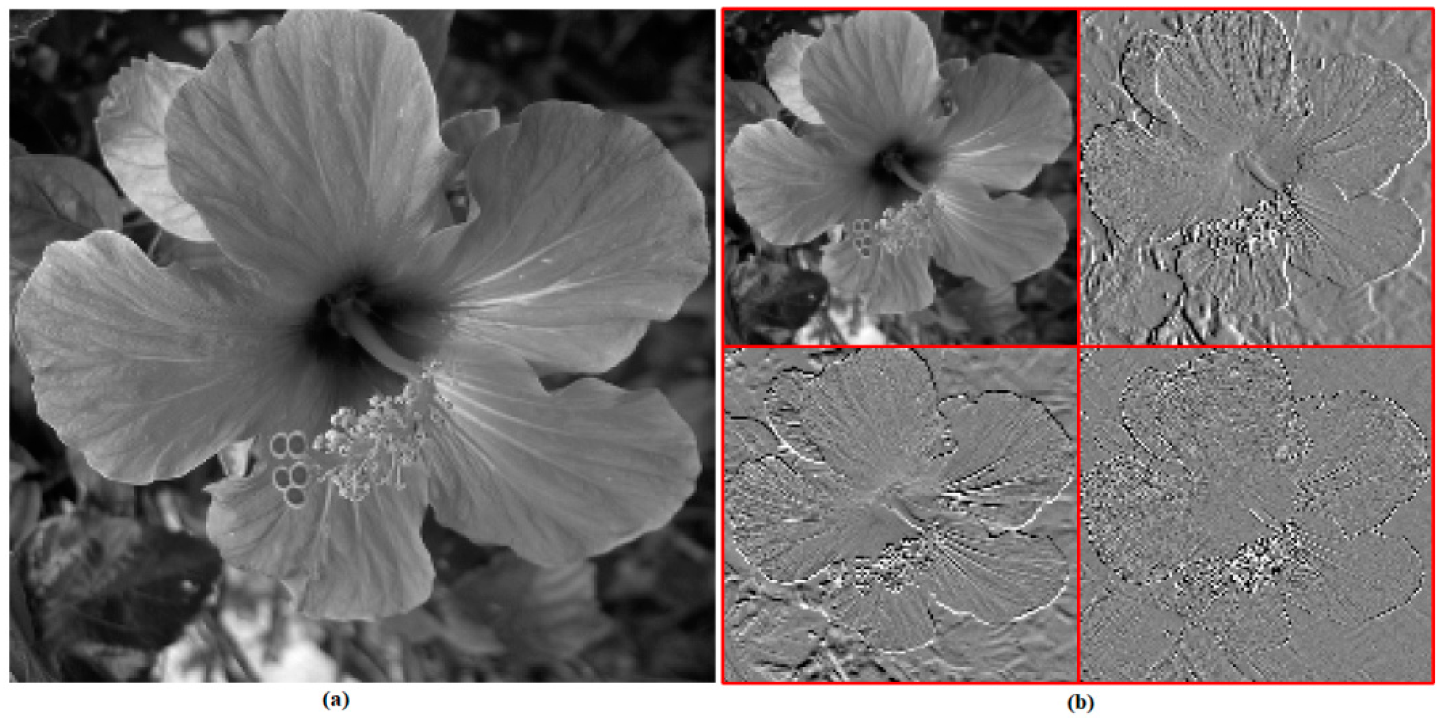
After getting the desired unknown wavelet coefficients, one-level inverse wavelet transform is required to get the desired HR output. Figure 2 shows the wavelet decomposition at level one of the hibiscus image. It can be seen from the image that a strong dependency is present between the wavelet coefficients at the given level and its sub-bands.

There have been several attempts to handle the problem of dimensionality reduction. In [34], authors propose a local linear embedded (LLE) approach that computes low-dimensional, neighborhood-preserving embeddings of high-dimensional inputs. The LLE approach maps its inputs into a single global coordinate system of lower dimensionality, and its optimizations do not involve local minima. LLE is able to learn the global structure of nonlinear manifolds, such as those generated by images of faces or documents of text. In [35], the authors describe an approach that combines the classical techniques of dimensionality reduction, such as principal component analysis (PCA) and multidimensional scaling (MDS) features. This approach is capable of discovering the nonlinear degrees of freedom that underlie complex natural observations, such as human handwriting or images of a face under different viewing conditions. In [36], authors have compared PCA, kernel principal component analysis (KPCA), and independent component analysis (ICA) to a support vector machine (SVM) for feature extraction. Furthermore, the authors described that the KPCA method is best among three for feature extraction. In [37], authors have proposed a geometrically motivated algorithm for representing the high-dimensional data, which provides a computational approach to dimensionality reduction compared to previous classical methods like PCA and MDS. The algorithm proposed learns a single network model for multiple scale-ups. However, the proposed algorithm utilizes the wavelet domain decomposition before the training of the network, and the wavelet sub-band images are used as the input the training. As can be seen from Figure 2, which shows the wavelet decomposition of a single image, the wavelet sub-band images are significantly sparse, and represent the directional fine features of the images. Further implying the dimensionality results will result in the loss of such directional fine features.

However, in spite of the sparsity property of the wavelets, the assumption of independence of wavelet coefficients at consecutive levels is somewhat limited for the task of SISR. This assumption fails to take into account the intra-scale dependency of the wavelet coefficients that capture the useful structures from the given images.

We make use of this dependency on the task of SISR. The proposed algorithm is different from the previous neural network- and wavelet domain-based methods in the following aspects.

• We use the SWT wavelet decomposition of the image and estimate the wavelet coefficients;
• We propose the deep network architecture similar to very deep super-resolution (VDSR) algorithm [18], but we train the network on the wavelet domain images instead of residual images—whereas, the authors of [16] utilize the DWT with a three-layer neural network inspired by SRCNN [8];
• We take a step further and design the deep network with 20 layers in the wavelet domain. The proposed wavelet-integrated deep-network (WIDN) model for super resolution estimates the sparse output, thus improving its reconstruction accuracy and training efficiency.

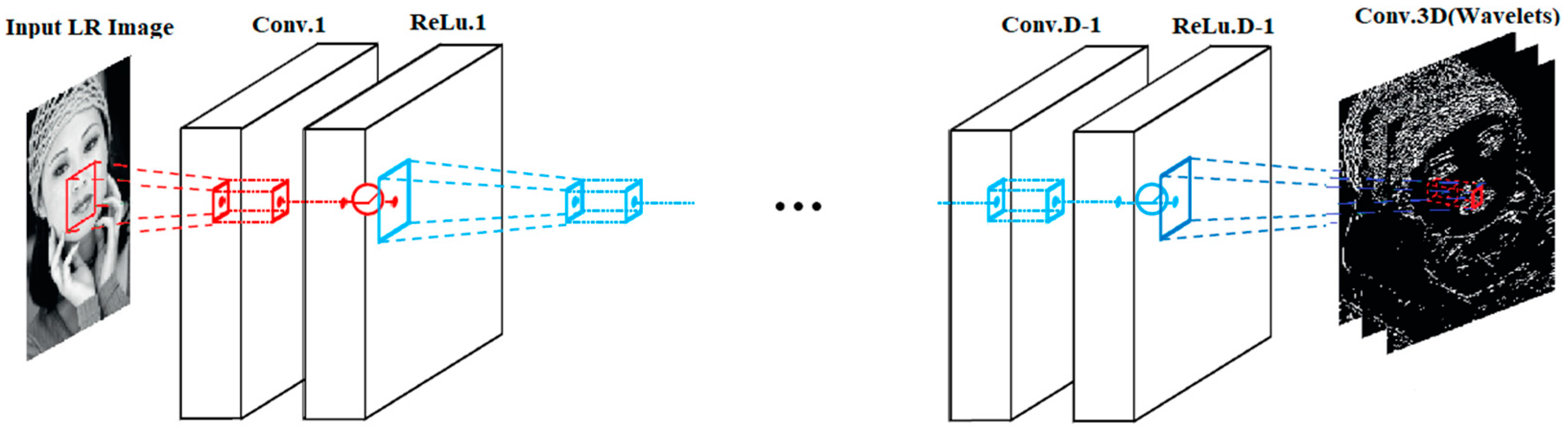
For the WIDN, the deep-network architecture is inspired by the Simonyan and Zisserman [38]. The network configuration can be found in Figure 3.

In our network model, we utilize D layers. All the layers in our network are the same except the first and the last. In our network, the first layer has a total of 64 filters. The size of each filter is 1 × 3 × 3 × 64. These filters operate at a 3 × 3 spatial size on 64 channels. These channels are also called feature maps. The first layer is used for the LR input image, and the last layer reconstructs the output image. As the last layer is used for the output image reconstruction, it has three filters, each of size 3 × 3 × 3 × 64. Our network is trained between the input LR image and its corresponding wavelet coefficients. Thus, given an input LR image, the network can predict the corresponding wavelet coefficients for HR image reconstruction. Modeling the image details in the wavelet domain has certain usefulness for the task of SISR [13,14,15]. The proposed model shows that by using wavelet details, the performance of SISR is highly improved. One of the problems pertaining to the deep convolution networks is that size of the output feature maps get reduced after each layer as the convolution operation is performed.

The problem is maintaining the same output size after each convolution operation is performed. Some authors suggest the use of surrounding pixels can give information about the center pixel [8]. This is quite handy when it comes to the problem of SISR. However, for the boundary of the image this can fail; cropping may be utilized to solve this problem. To alleviate the problem of size reduction and boundary condition, we employed zero paddings before the convolution operation. We find that by doing so, the size of the features remains constant, and the boundary condition problem is also solved. Once the three wavelet sub-bands are predicted, we add back the LR input image and do one-level wavelet reconstruction to get the HR image estimate.

Data preprocessing is a very important step to make features invariant to input scale and reduce dimensionality in the machine learning process (a restricted Boltzmann machine, or RBM), which is likely to be used for preprocess the input data. In [39], the authors note that the RBM is an undirected graphical model with hidden variables and visible variables along with a feature learning approach, which is used to train an RBM model separately for audio and video. After learning the RBM, the posteriors of the hidden variables given the visible variables can be used as a new representation of the data. This model is used for multimodal learning as well as for pre-training the deep networks. In [40], the authors present the sparse feature representation method based on unsupervised feature learning. By using the RBM graphical model, which consists of visible nodes and hidden nodes, the visible nodes represent input vectors, while hidden nodes are feature-learned by training the RBM. This method helps to pre-process the data. In [41], the authors present a method in which a number of motion features computed by a character’s hand is considered. The motion features are preprocessed using restricted Boltzmann machines (RBMs). RBM pre-processing performs a transformation of the feature space based on an unsupervised learning step. In our proposed model, we have utilized the data augmentation technique for pre-processing the data, inspired by VDSR [18] and FSRCNN [21] algorithms. However, implementing the RBMs will definitely be considered as a future task of our approach.

3.1. Training

For the training of our model, we require a set of HR images. As we train our model between the wavelet approximation image and its corresponding sub-band coefficient images, we do a one-level wavelet decomposition on the HR images from the training data set. The wavelets have a very unique property of redundancy across the scale.

Given the wavelet approximation image at a certain scale and its coefficients, one can perfectly reconstruct the preceding approximation image. Thus, the wavelet coefficient contains all the information about the preceding approximation image. We utilize this property of the wavelet and learn the mappings between the wavelet approximation image and its corresponding coefficients for the task of SISR. Let X denotes the level1 wavelet LR image and Y denote the detail sub-band images. The task is to learn the relationship between the LR approximation image and its corresponding same-level wavelet sub-band images (horizontal, vertical, and diagonal).

In the algorithm SRCNN [8], one problem is that the network has to preserve the information about input details as the output is obtained, using these learned features alone, and the input image is not utilized and discarded. If the network is deep, having many weight layers, this corresponds to an end-to-end learning problem, which requires a huge memory.

Due to this reason, the problem of the vanishing/exploding gradient [42] arises and needs to be solved. We can solve this problem by wavelet coefficient learning. As we assume the dependency between the wavelet LR approximation image and its corresponding same-level detailed coefficients, we define the loss function as

$$\mathrm{L}\left(\mathsf{\Theta }\right)=\frac{1}{\mathrm{k}}{{\displaystyle \sum }}_{\mathrm{i}=1}^{\mathrm{k}}({{\displaystyle \sum }}_{\mathrm{b}=1}^3||\mathrm{f}{({\mathrm{X}}_{\mathrm{i},}\mathsf{\Theta })}^{\mathrm{b}}-{\mathrm{y}}_{\mathrm{i}}^{\mathrm{b}}||),$$

(6)

where k is the number of training samples, X is the tensor containing the LR approximation images, and Y is the tensor containing the wavelet sub-band images (horizontal, vertical, and diagonal). T represents the network parameters, and b represents the sub-band index. For the training, we use the gradient descent-based algorithm from [43]. This algorithm works on the mini-batch of images and utilizes the back-propagation approach to optimize the objective function. In our model, we set the momentum parameter to be 0.9, with the regularizing penalty on the weight decay as 0.0001. Now, to boost the speed on training, one can use a high learning rate. However, if a high learning rate is utilized, the problem of vanishing/exploding gradients [42] becomes evident. To solve this, we utilize the adjustable gradient clipping.

Gradient Clipping

Gradient clipping is generally used for training the recurrent neural networks [38]. However, it is seldom used in the CNN training. There are many ways in which gradients can be clipped. One of them can be to clip them in a pre-defined range $\left(-\mathsf{\theta },\mathsf{\theta }\right)$. In the process of clipping, the gradient lies in a specific range. If the stochastic gradient descent (SGD) algorithm is used for training, we multiply the gradient with the learning rate for step size adjustment. If we want our network to train much faster, we need a high rate of learning; to achieve this value, the gradient $\mathsf{\theta }$ must be high.

However, high gradient values will cause the exploding gradients problem. We can avoid this problem by using a smaller learning rate. However, if the learning rate is made smaller, the effective gradient approaches zero, and the training may take a lot of time. For this purpose, we propose to clip the gradients to $\left[-\frac{\mathsf{\theta }}{\mathsf{\gamma }},\frac{\mathsf{\theta }}{\mathsf{\gamma }}\right]$, where $\mathsf{\gamma }$ is the learning rate. By doing so, we observe that the convergence of our network becomes faster. It is worth mentioning here that our network converges within 3 h, just like in [44], while the SRCNN [16] takes several days to train. Despite the fact that the deep models proposed nowadays have greater performance capability, if we want to change the scale-up the parameter, the network is trained for that scale again, and hence for each scale, we need a different training model.

Considering the fact that the scale factor is used often and is important, we need to find a way across this problem. To tackle this problem, we propose to train a multi-scale model. By doing so, we can utilize the parameters and features from all scales jointly. To do so, we combine all the approximation images and their corresponding wavelet sub-bands across all predefined scale factors, and form a big data set of training images.

4. Properties of the Proposed Model

Here we discuss the properties of the proposed model. First, we say that the large depth networks can give good performance for the task of SISR. Very deep networks make use of the contextual information of an image, and can model complex functions with many non-linear layers. We experimentally validate our claim. Second, we argue that the proposed network gives a significant boost in performance, with an approximately similar convergence speed to VDSR.

4.1. Deep Network

Convolution neural networks make use of the spatial–local correlation property. They enforce the connecting patterns between the neurons of adjacent layers in the network model. In other words, for the case of hidden units, the output from the layer m − 1 is an input to the layer m in the network model. By doing so, a receptive field is formed that is spatially contagious. In this network model, the corresponding hidden unit in the network only corresponds to the receptive field, and is invariant to the changes outside its receptive field. Due to this fact, the filters learned can efficiently represent the local spatial patterns in the vicinity of the receptive field.

However, if we stack a number of such layers to form a network model, the output ends up being global—i.e., it corresponds to bigger pixel space. The other way around, a filter having large spatial support can be broken into a number of filters with smaller spatial support. Here we use 3 × 3 size filters to learn the wavelet domain mappings. The filter size is kept the same for all corresponding layers. This means that the receptive field for the layer has the 3 × 3 filter size. For the corresponding proceeding layer, this size is increased by a factor of two. The depth of the receptive field in our model has the size of (2D + 1) × (2D + 1). For the task of SISR, if one has more contextual information about the high-frequency components, it can be used to infer and generate a high-quality image. In this paradigm of neural networks, a bigger receptive field can serve the purpose of extracting more contextual information. As the problem of super-resolution is highly ill-posed, using more contextual information is bound to give better results.

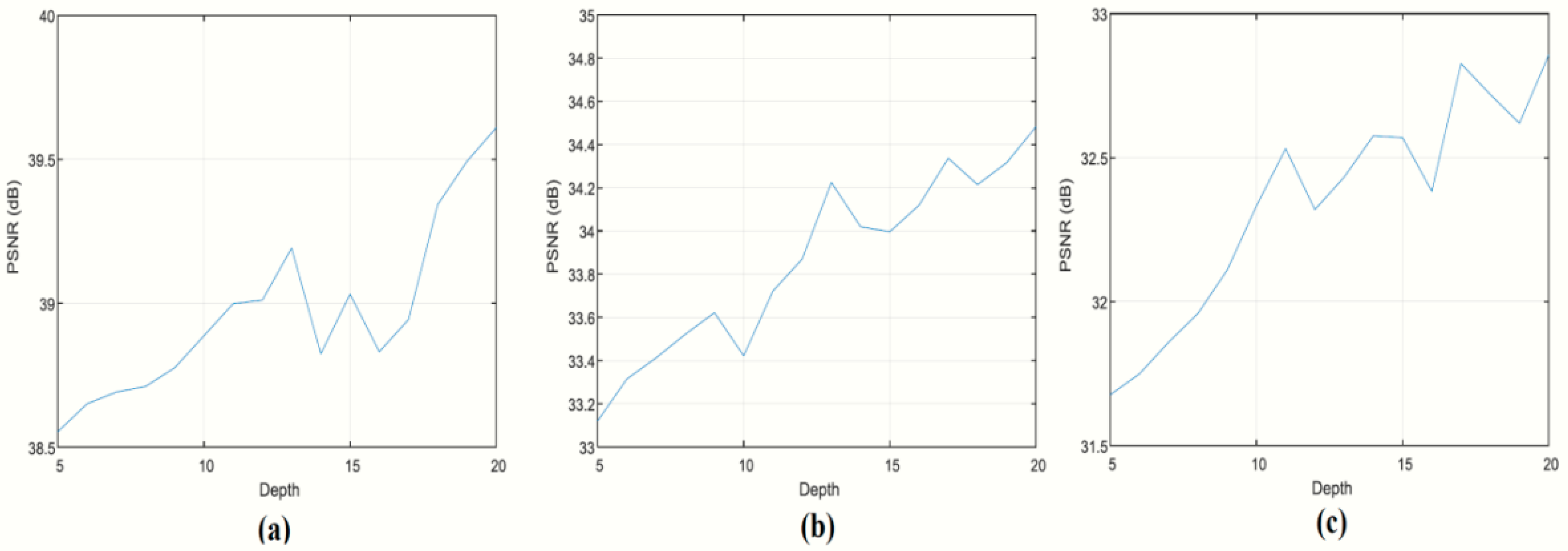
Another advantage of using deep networks is that they can model non-linearity very well. In our proposed network architecture, we utilize 19 ReLUs, which allows our network to model highly complex non-linear functions. We experimentally evaluated the performance of deep networks by calculating the network’s PSNR as depth values increased from 5 to 20, only counting the weight layers and excluding the non-linearity layers. The results are shown in Figure 4. In most cases, the performance increases as depth increases.

There are a number of different techniques in machine learning to solve computational problems. Some of them we discuss here and compare with our proposed WIDN. In [45], authors have proposed a recurrent neural network (acRNN), which synthesizes highly complex human motion variations of arbitrary styles, like dance or martial arts, without asking from the database. In [46], the authors have proposed dilated convolutional neural network for capturing temporal dependencies in the context of driver maneuver anticipation. In [47], authors have proposed CNN for speech recognition within the framework of a hybrid NNHMM model. Hidden Markov models (HMMs) are used in state-of-the-art automatic speech recognition (ASR) to model the sequential structure of speech signals, where each HMM state uses a Gaussian mixture model (GMM) to model a short-time spectral representation of the speech signal. In [48], authors have briefly explained in detail the number of graphical models that can be used to express speech recognition systems. The main idea of the proposed work is the wavelet domain-based deep-network algorithm. In our proposed model, we use the wavelet sub-band images as the input to the network, and learn a single model for multiple degradations. One can try such an implementation with other DNN-based algorithms, but the first one needs to investigate whether the DNN will be compatible with the wavelet sub-band images or itself. One also has to account for the sparsity and directionality of the wavelet sub-band images. We have proposed the DNN model of the VDSR [18] algorithms, as it utilizes the residual images obtained by subtracting the LR from HR images for the training of the network. The wavelet sub-band images possess quite similar properties as the residual images for the task of SISR. Experimental analysis validated our assumption, and comparative analysis proved the efficacy of the proposed model.

4.2. Wavelet Learning

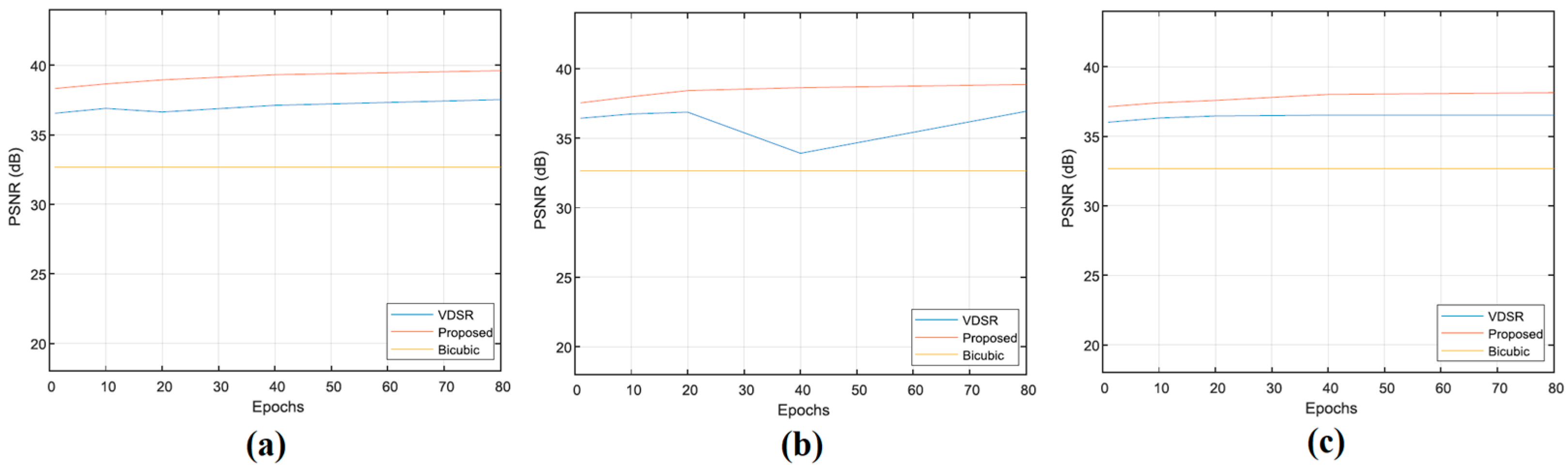
In this work, we propose a network structure that learns wavelet sub-band images. We now study this modification to the VDSR approach. First, we show that for approximately similar convergence, the network gives better performance. We use a depth of 20(weight layers) and the scale parameter is 2. Performance curves for various learning rates are shown in Figure 5. All use the same learning rate scheduling. It can be seen that the proposed algorithm gives superior performance.

5. Experiments and Results

Here we give the details about the experiments and results. Data preparation in our case is similar to SRCNN [8], with a minute difference. In our model, the patch size of the input image is made the same as the receptive field of the network. We do not utilize the overlap condition while extracting the patches to form a mini-batch. A single mini-batch in our model has a total of 64 sub-images. Also, the sub-images corresponding to the difference scales can also be combined to form a mini-batch. We implement our model using the publicly available MatConvNet package [44]. For the training data set, we used the 291 images with augmentation (rotations), as done in [21].

For the test data sets, we used the most commonly used data sets of “Set5”, “Set14”, “Urban100”, and “BSD100”, as used in previous works [18,21,23,24]. The depth of our network model is 20. The batch size used is 64. The momentum used is 0.9 with the decay rate of 0.0001. The network was trained for 80 epochs, and initially, the learning rate was set to 0.1; after every 20 iterations, we decreased it by a factor of 10. The training of our model normally takes about 3 h using the GPU Titan Z. However, if we use a small training set like that in [49], we can increase the speed of learning.

Table 1. Performance table (peak signal-to-noise ratio, or PSNR) for the proposed and VDSR [18] networks (“Set5” dataset, ×2).

(a) 0.1 rate of learning
Epoch	VDSR [18]	Proposed	Difference
10	36.90	38.66	1.76
20	36.64	38.95	2.31
40	37.12	39.32	2.20
80	37.53	39.61	2.08
(b) 0.01 rate of learning
Epoch	VDSR [18]	Proposed	Difference
10	36.82	37.98	1.16
20	36.90	38.42	1.52
40	36.98	38.63	1.65
80	37.06	38.86	1.8
(c) 0.001 rate of learning
Epoch	VDSR [18]	Proposed	Difference
10	36.42	37.41	0.99
20	36.58	37.58	1
40	36.69	38.01	1.32
80	36.79	38.13	1.34

shows the average PSNR values of the proposed algorithm with increasing numbers of epochs and on different learning rates. It can be seen from the Table 1 that the proposed algorithm provides good results by employing the deep neural network architecture in the wavelet domain.

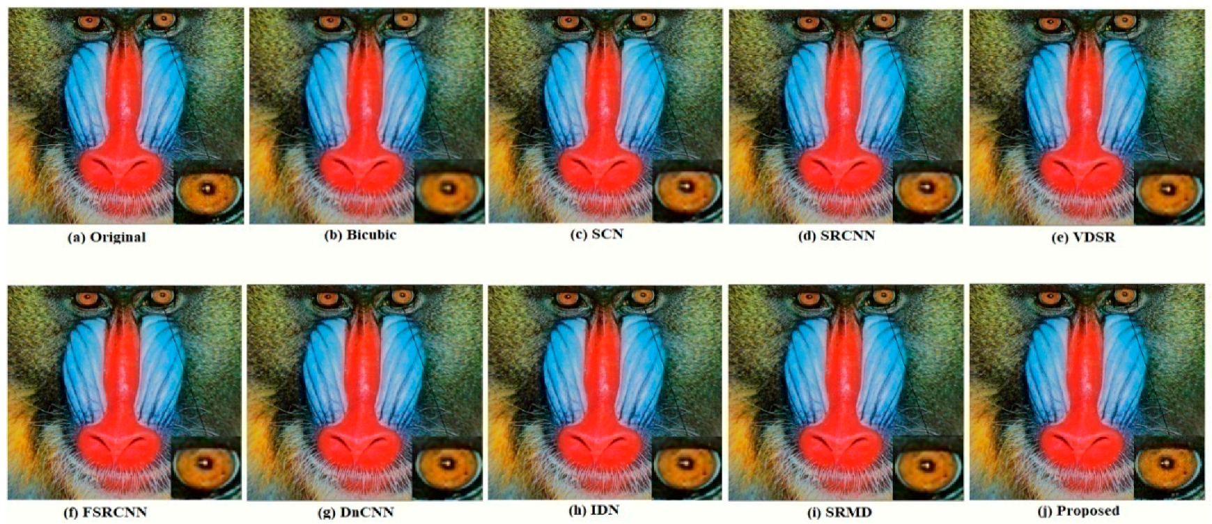
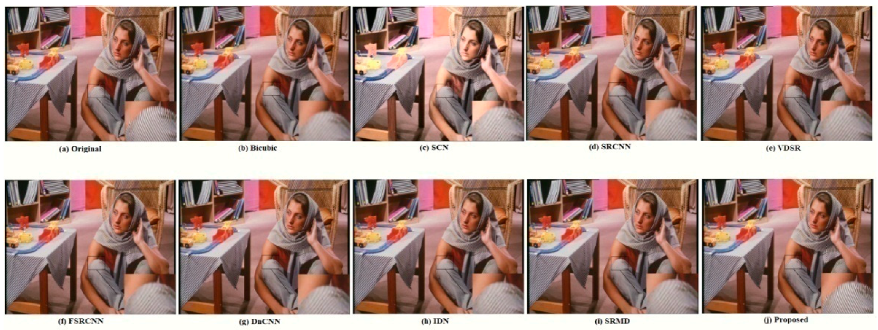
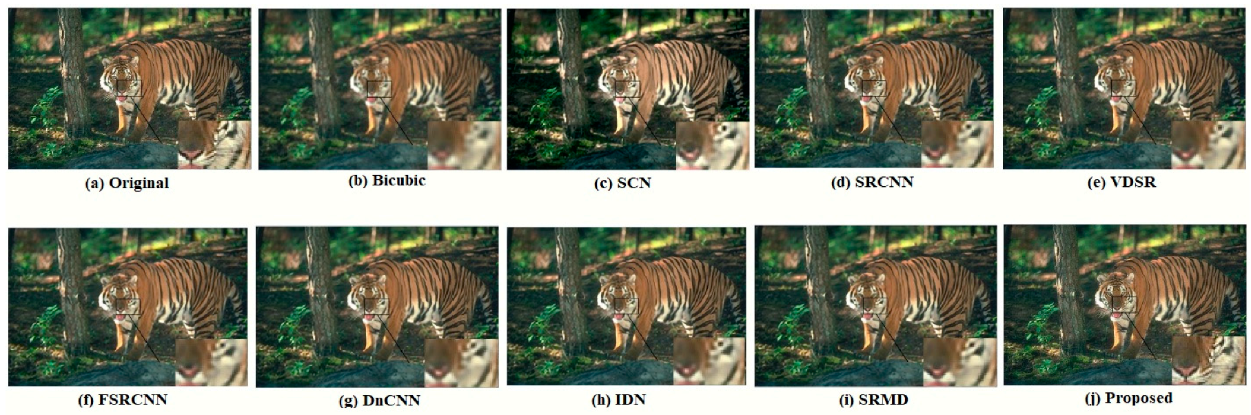
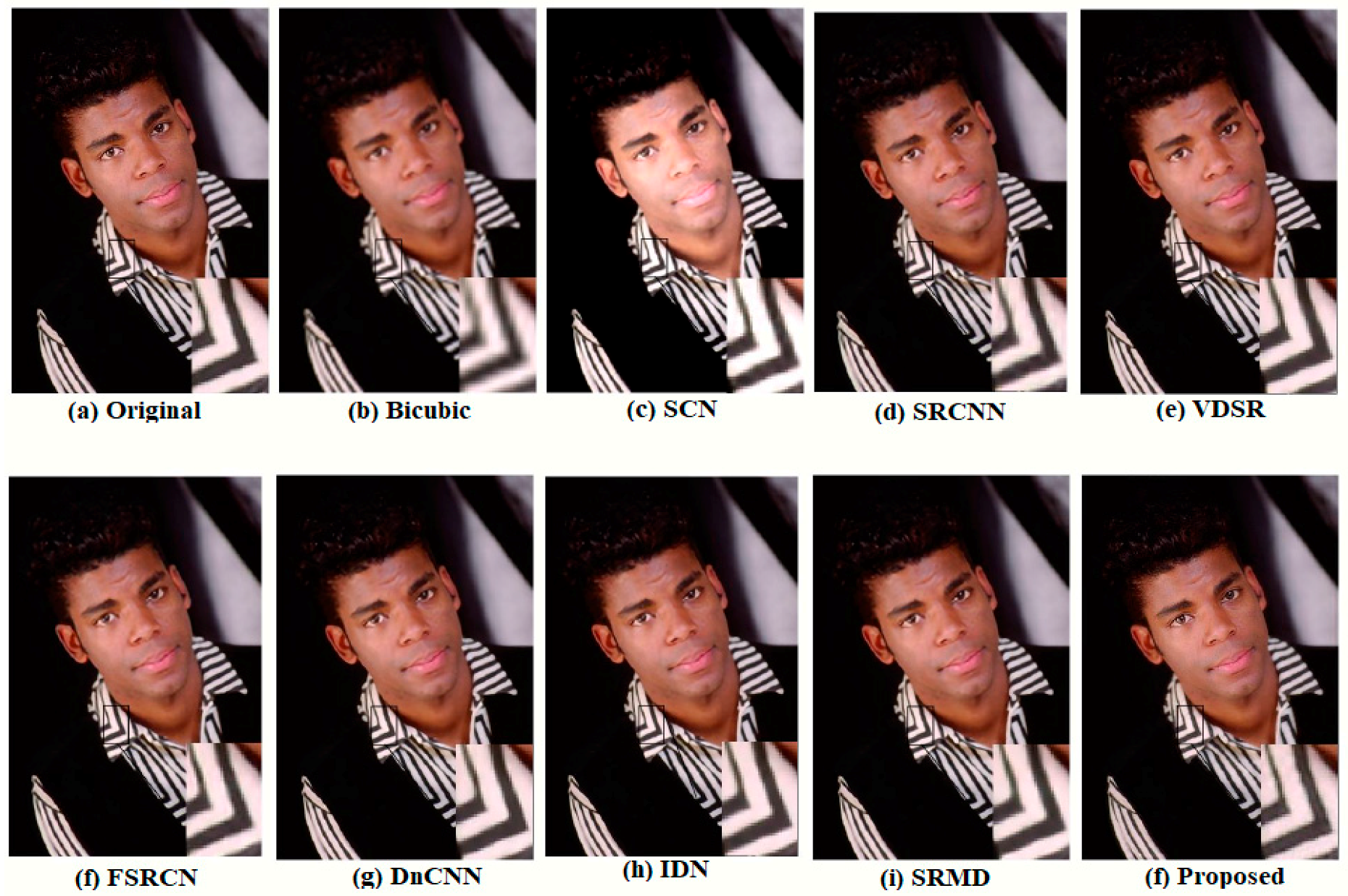
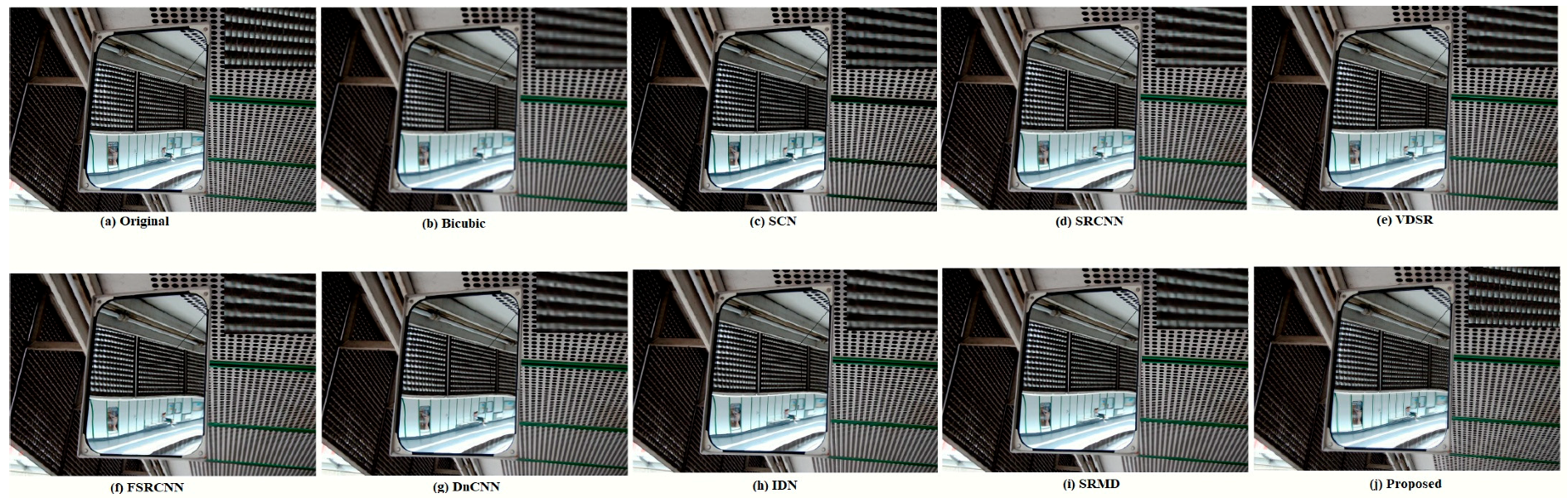
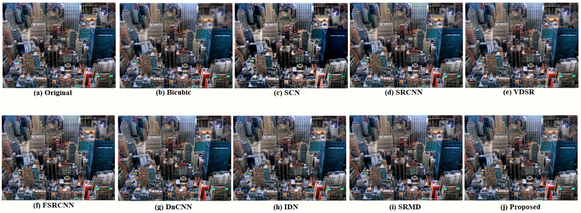
The visual results are shown in Figure 6, Figure 7, Figure 8, Figure 9, Figure 10 and Figure 11. Figure 6 and Figure 7 show the comparative results for the scale-up parameter of 2. Almost all the algorithms perform better. However, the proposed wavelet domain-based algorithm provides more sharp edges and textures. Figure 8 and Figure 9 show the comparative results from the BSD100 test set images for the scale-up parameter of 3.

Here the algorithms under comparison fail to provide good results; however, the proposed algorithm provides better results. Figure 10 and Figure 11 are taken from a more challenging image data set of Urban100. Here, the scale-up parameter used is 4. Looking at Figure 10 and Figure 11, the proposed algorithm is able to recover the sharp edges and texture where other algorithms fail.

The quantitative analysis based on PSNR and SSIM is shown in

Table 2. Comparative results based on PSNR (left) and the structural similarity index measure (SSIM) (right).

Data Set	Scale	Bicubic	SRCNN [8]	SCN [11]	VDSR [18]	DnCNN [22]	FSRCNN [21]	SRMD [24]	IDN [23]	Proposed
Set 5	2	33.64/0.929	36.35/0.953	36.52/0.953	37.56/0.959	37.58/0.959	36.99/0.955	37.53/0.959	37.83/0.960	39.60/0.983
	3	30.39/0.866	32.74/0.908	32.60/0.907	33.67/0.922	33.75/0.922	33.15/0.913	33.86/0.923	34.11/0.952	34.48/0.943
	4	28.42/0.810	30.48/0.863	30.39/0.862	31.35/0.885	31.40/0.884	30.71/0.865	31.59/0.887	31.82/0.890	32.85/0.929
Set 14	2	30.22/0.868	32.42/0.906	32.42/0.904	33.02/0.913	33.03/0.912	32.73/0.909	33.12/0.914	33.30/0.915	34.44/0.980
	3	27.53/0.774	29.27/0.821	29.24/0.819	29.77/0.832	29.81/0.832	29.53/0.826	29.84/0.833	29.99/0.835	30.95/0.931
	4	25.99/0.702	27.48/0.751	27.48/0.751	27.99/0.766	28.04/0.767	27.70/0.756	28.15/0.772	28.25/0.773	29.75/0.909
BSD100	2	29.55/0.843	31.34/0.887	31.24/0.884	31.89/0.896	31.90/0.896	31.51/0.891	31.90/0.896	32.08/0.898	33.52/0.979
	3	27.20/0.738	28.40/0.784	29.32/0.782	28.82/0.798	28.85/0.798	28.52/0.790	28.87/0.799	28.95/0.801	29.99/0.928
	4	25.96/0.667	26.90/0.710	26.87/0.710	27.28/0.726	27.29/0.725	26.97/0.714	27.34/0.728	27.41/0.730	28.10/0.910
Urban 100	2	26.66/0.841	29.53/0.897	29.50/0.896	30.76/0.914	30.74/0.913	29.87/0.901	30.89/0.916	31.29/0.920	32.48/0.952
	3	24.46/0.737	26.25/0.801	26.21/0.801	27.13/0.828	27.15/0.827	26.42/0.807	27.27/0.833	27.42/0.846	28.68/0.941
	4	23.14/0.653	24.52/0.722	24.52/0.725	27.17/0.753	25.20/0.752	24.67/0.727	25.34/0.761	25.41/0.763	26.41/0.903

. The algorithms under comparison include the bicubic technique, SRCNN algorithm [8], SCN algorithm [11], VDSR algorithm [18], FSRCNN algorithm [21], DnCNN algorithm [22], IDN algorithm [23], and SRMD algorithm [24]. In the comparative analysis, the trained models used for these algorithms are provided by the authors. The proposed algorithm gives better results than the algorithms under comparison.

6. Conclusions

A scale-invariant, wavelet-integrated deep-network model is proposed for the task of SISR. To improve the training speed of the algorithm, the adjustable gradient clipping is used. Useful properties of the convolution neural networks, such as large model capacity, end-to-end learning, and high performance, are exploited in the wavelet domain for the task of SISR. The up-sampling SWT is proposed instead of the down-sampling DWT, to avoid the data loss. Experimental analysis is carried out to validate the efficacy of the proposed model. Quantitative results based on the PSNR and SSIM indicate that the proposed algorithm performs better in comparison with the recent state-of-the-art algorithm. Visual results also validate the quantitative ones. The proposed algorithm can be extended and modified for other super-resolution applications, such as face and brain image enhancement. Also, the proposed algorithm can be tested with other wavelet transforms, such as dual-tree complex wavelet transforms (DT-CWT).