Pansharpening with a Gradient Domain GIF Based on NSST

Abstract

In order to improve the fusion quality of multispectral (MS) and panchromatic (PAN) images, a pansharpening method with a gradient domain guided image filter (GIF) that is based on non-subsampled shearlet transform (NSST) is proposed. First, multi-scale decomposition of MS and PAN images is performed by NSST. Second, different fusion rules are designed for high- and low-frequency coefficients. A fusion rule that is based on morphological filter-based intensity modulation (MFIM) technology is proposed for the low-frequency coefficients, and the edge refinement is carried out based on a gradient domain GIF to obtain the fused low-frequency coefficients. For the high-frequency coefficients, a fusion rule based on an improved pulse coupled neural network (PCNN) is adopted. The gradient domain GIF optimizes the firing map of the PCNN model, and then the fusion decision map is calculated to guide the fusion of the high-frequency coefficients. Finally, the fused high- and low-frequency coefficients are reconstructed with inverse NSST to obtain the fusion image. The proposed method was tested using the WorldView-2 and QuickBird data sets; the subjective visual effects and objective evaluation demonstrate that the proposed method is superior to the state-of-the-art pansharpening methods, and it can efficiently improve the spatial quality and spectral maintenance.

1. Introduction

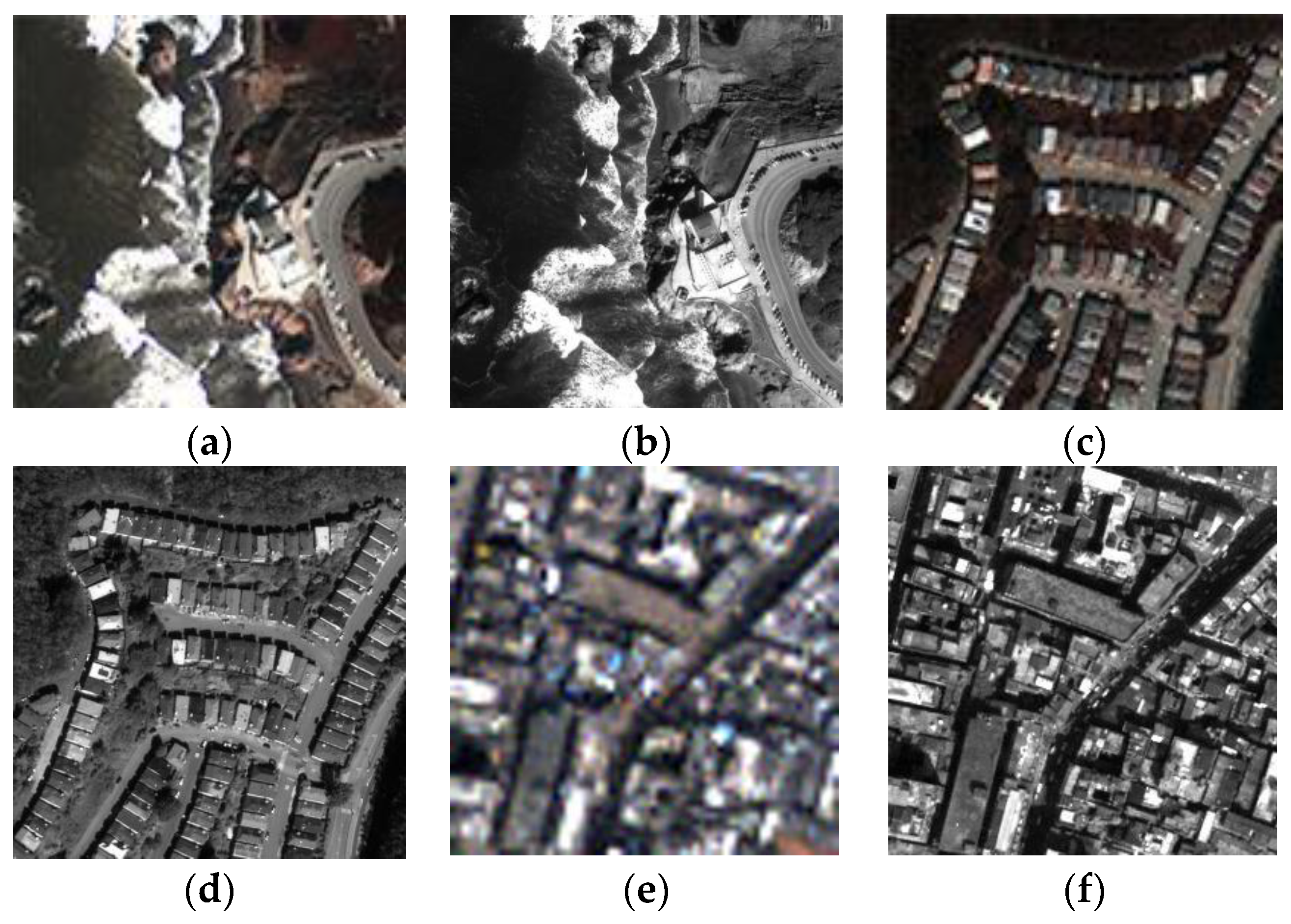
With the development of satellite technology and imaging systems, we are able to obtain remote sensing images with higher resolution. High-resolution remote sensing images can describe target information more accurately, which is of great significance in the development of numerous applications, such as environmental monitoring, land and resource planning, military mapping, object recognition, and scene interpretation. Most commercial satellites, such as QuickBird, IKONOS, GeoEye, and WorldView, can currently jointly obtain panchromatic (PAN) and multispectral (MS) images. Due to imaging physical constraints and transmission bandwidth limit, it has been difficult to obtain images with the characteristics of both high spatial resolution and high spectral resolution. Fusion is one of the most important and effective methods in providing better interpretation ability of remote sensing images. How to combine complementary information of PAN and MS images is an urgent problem to be solved.

MS images have the advantage of high spectral resolution, while PAN images have the advantage of high spatial resolution. The purpose of fusion is to combine the complementary characteristics of the original images and provide enough information for image interpretation. The component substitution (CS) method is a traditional pansharpening model, which includes intensity-hue-saturation transformation (IHS) [1], principle component analysis (PCA) [2], the Gram-Schmidt process (GS) [3], and so on. These methods offer outstanding spatial quality but they have the problem of serious spectral distortion in the fused image. The CS method has been extended and improved based on new theories over time, because of low computational complexity, [4,5]. In [6], an adaptive image fusion method that is based on the concept of partial replacement of intensity component is proposed, which is known as partial replacement adaptive CS (PRACS). A context-adaptive (CA) pansharpening method that is based on image segmentation is proposed in [7], which is integrated into the GS scheme in order to achieve a better estimation of the injection coefficients. The band-dependent spatial-detail (BDSD) model is also known as adaptive CS [8]. Model-based methods have gathered increasing interest in recent studies. This kind of method based on complex models can achieve a better pansharpening effect in some cases, but the time complexity is high due to the optimization process. Within this family, many contributions that are based on Bayesian methods rely on the sparse representations of signals [9,10] and total variation penalization [11,12] terms. Essentially, this can be regarded as a strategy of image repair, which consists of the reconstruction of the high-resolution MS image from the original data [13]. Multi-resolution analysis (MRA) methods, which decompose the image into different frequency coefficients, can harmonize the injection of spatial details and maintenance of spectral information. The MRA scheme is based on the injection of detailed information that is extracted from the decomposition coefficients of PAN images into the low-resolution MS bands. Wavelet transform is one of the MRA methods and it is an important milestone in the field of image processing as a mathematical tool [14]. The fusion results of wavelet transform provide certain improvements in preserving spectral information, but they also have shortcomings, such as direction limitation, shift, and aliasing. When compared with discrete wavelet transform (DWT), dual-tree complex wavelet transform (DTCWT) [15] has the advantages of shift-invariance and directional selectivity, but its limited number of directional textures and edges of wavelet families make it difficult to represent two-dimensional (2-D) images. To solve this problem, a number of multi-scale geometric analysis tools, such as curvelet transform [16], contourlet transform [17], and shearlet transform [18], have been developed and successfully applied to the pansharpening problem. 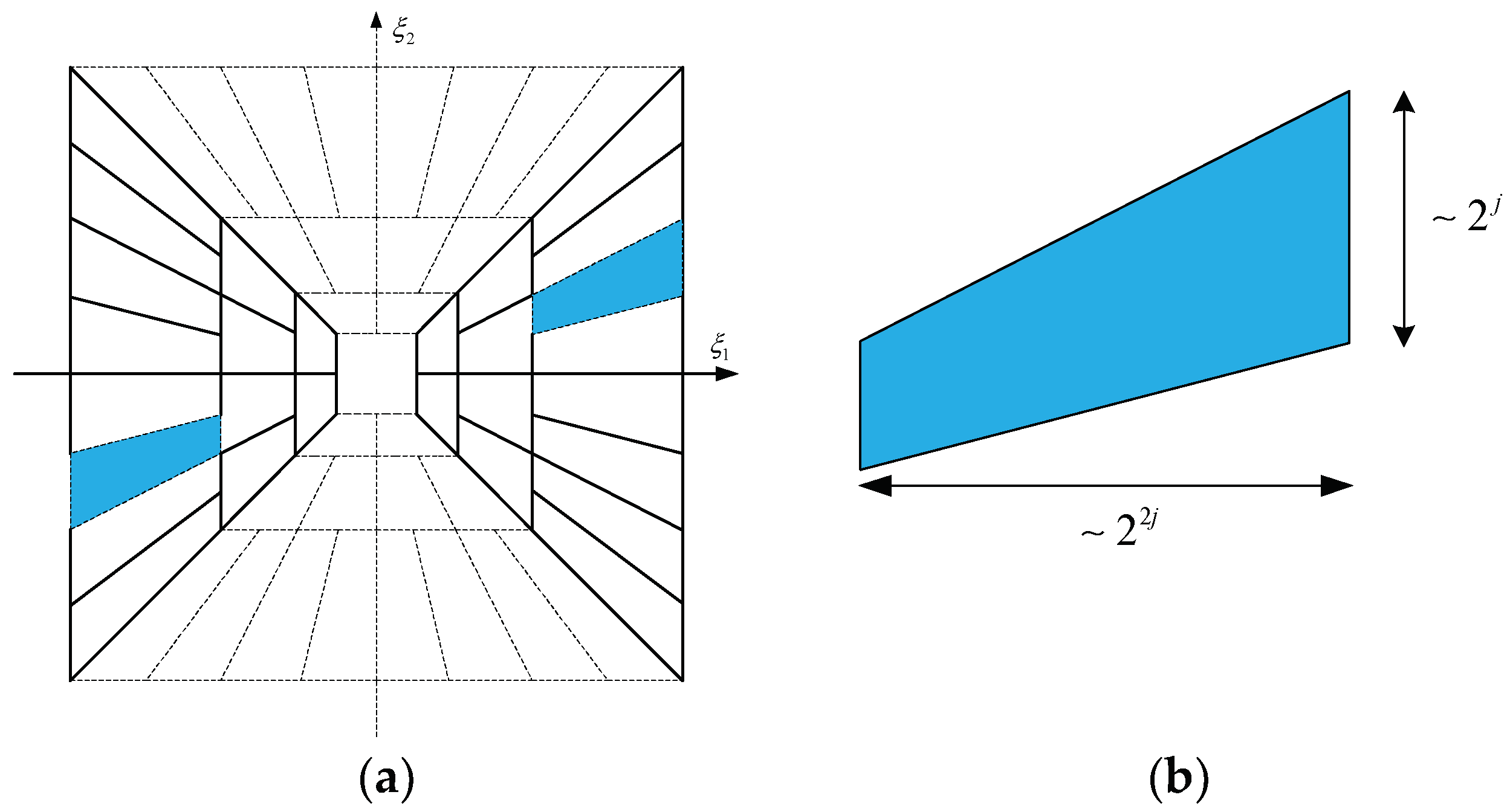The main motivation of multi-scale geometric analysis methods is to pursue a “true” 2-D transform [19], which can effectively capture the geometric structure of an image, so that the fusion quality can be further improved. However, without the shift-invariant property, the contourlet and shearlet transform may suffer the frequency alias problem. The non-subsampled contourlet transform (NSCT) [20,21] is an effective solution to this problem, but its application is limited by the finite decomposition directions and high computational complexity. Non-subsampled shearlet transform (NSST) is a shift-invariant version of shearlet transform, which attains a low computational cost and good image sparse representation performance [22]. For the current study, the appearance of NSST has provided a new solution for the pansharpening issue. As a novel multi-scale geometric analysis method, NSST is one of the topics that are currently being studied by many researchers. Moonon [23] proposed a remote sensing image fusion method based on NSST and sparse representation. Wu proposed a method that is based on improved non-negative matrix decomposition in the NSST domain [24] and a fusion method using chaotic bee colony optimization in the NSST domain [25]. Yang [26] proposed a pansharpening framework based on the matting model and multi-scale transform. These methods have good effects on pansharpening, although they all are subject to their own limitations.

The lack of an anti-aliasing feature in multi-scale decomposition tends to cause decision bias in the boundary region of objects. The bias will result in an artificial texture and image non-uniformity, and it therefore causes a bad influence on visual effects and image interpretation. In order to solve this problem, some spatial techniques and optimization strategies have been introduced into the fusion method, such as bilateral filter [27], cross bilateral filter (CBF) [28], weighted least squares filter [29], and guided image filter (GIF) [30,31]. The GIF is one of the fastest edge-preserving local filters and it is superior to bilateral filters in avoiding gradient reversal. 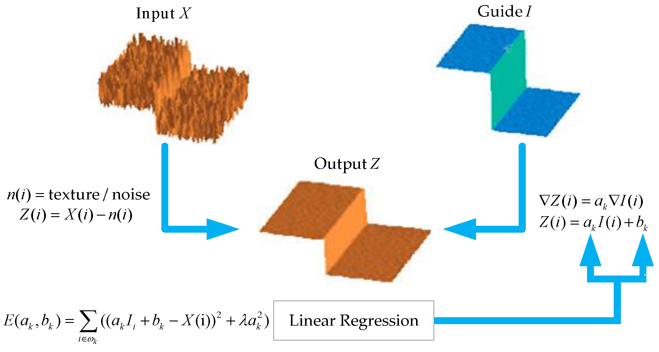Meng [32] proposed a pansharpening method with an edge-preserving guided filter based on three-layer decomposition and the decomposed PAN image is injected into the MS image within this method. However, due to the fixed regularized values in the GIF, the edges will inevitably be smoothed. Li [33] proposed a weighted GIF, which avoided the edge blurring problem to some extent. However, these two methods do not have explicit constraints in processing the edges of images and the filtering process is usually accompanied by image coarsening. When both edge preservation and filtering are considered, the problem of edge blurring will inevitably occur. Moreover, in some cases, these methods still cannot maintain the edges well, which leads to the degradation of fusion quality. Kou [34] proposed a gradient domain GIF, in which the introduction of explicit first-order edge condition constraints defines a new edge-perception weight, so that the edges of an image can be better preserved.

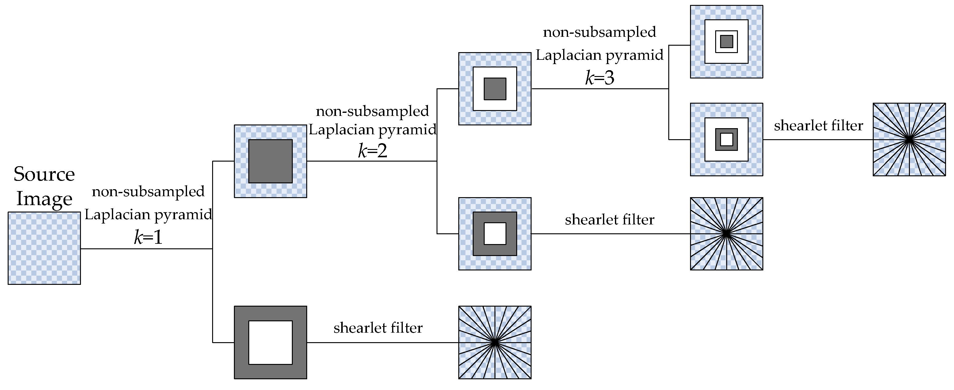
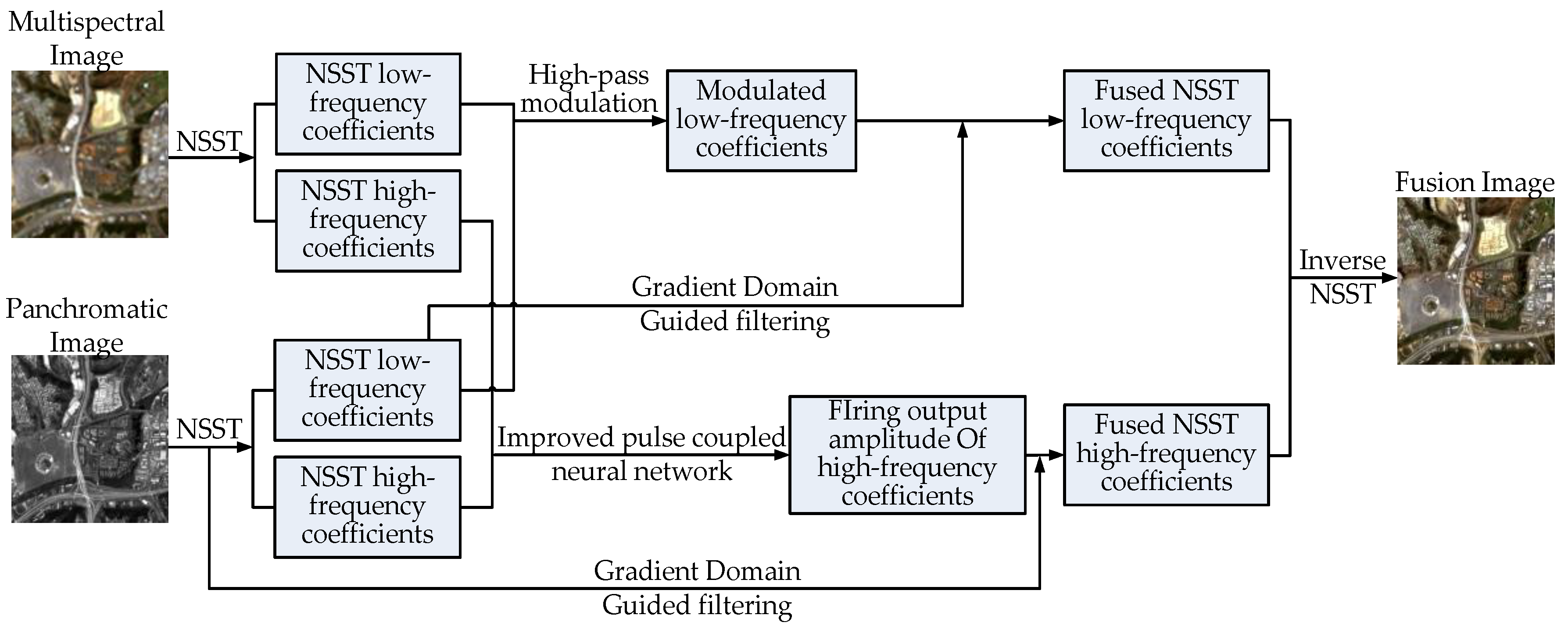
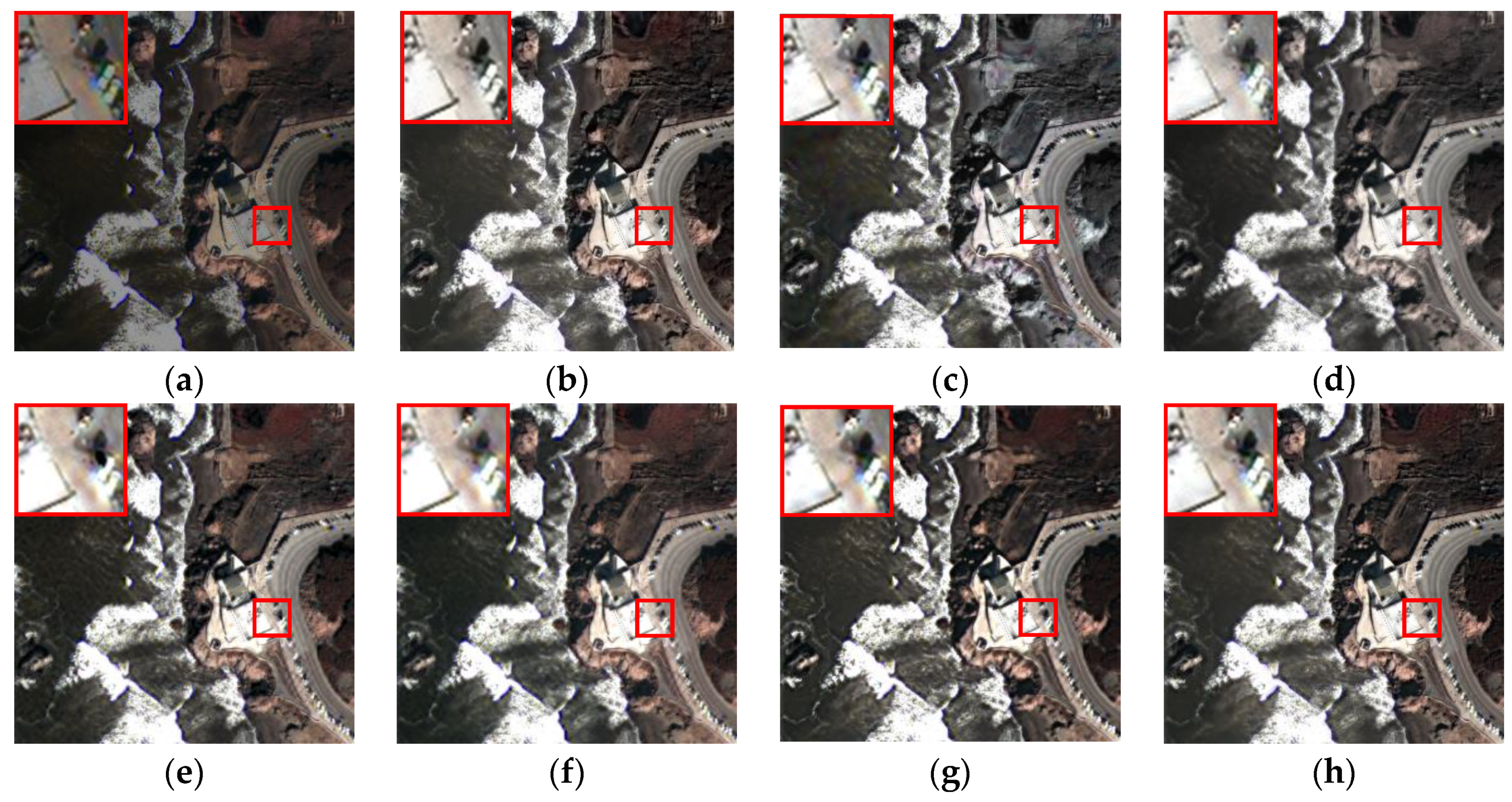
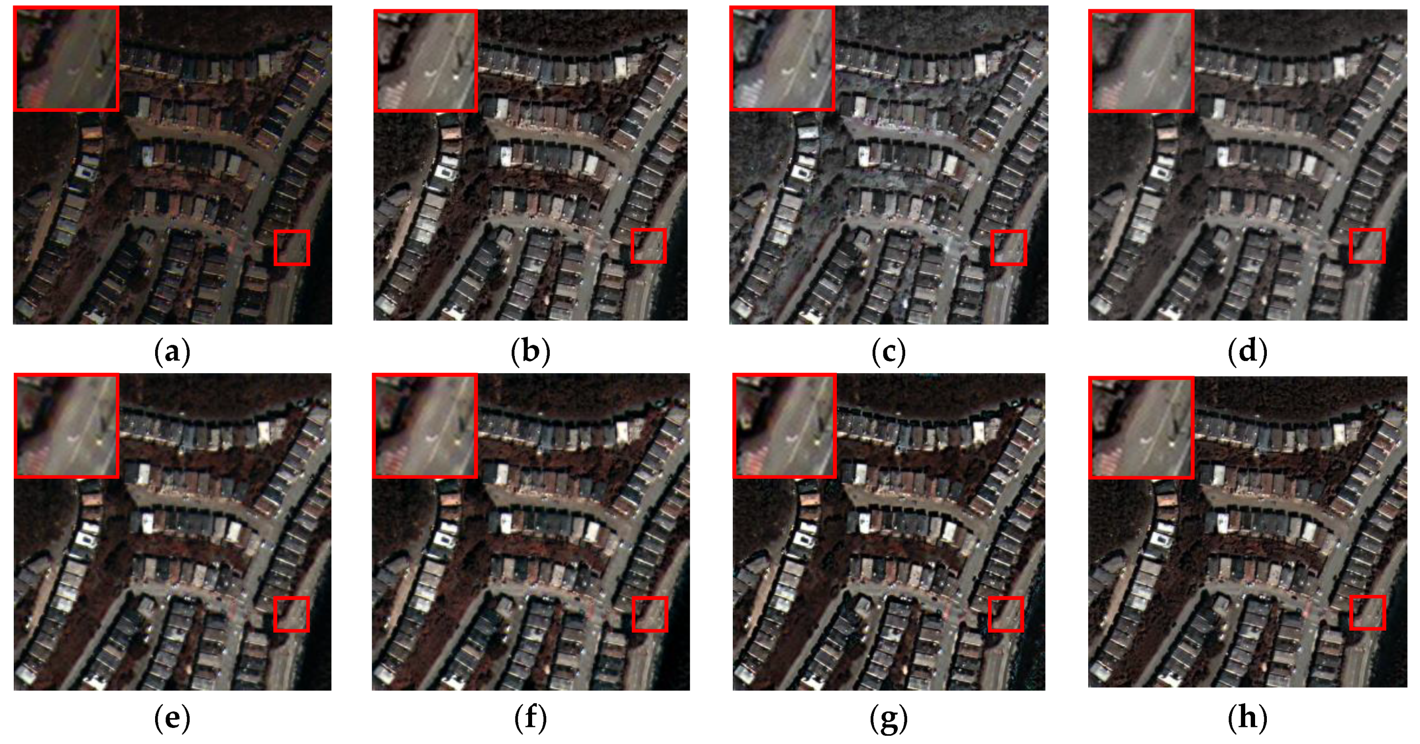
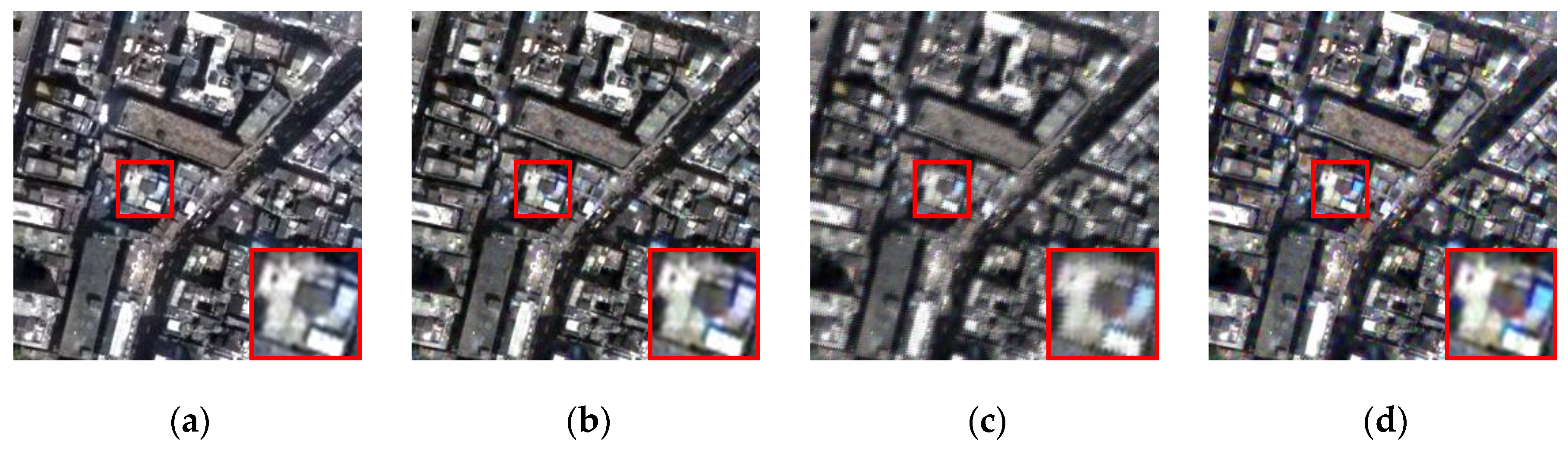
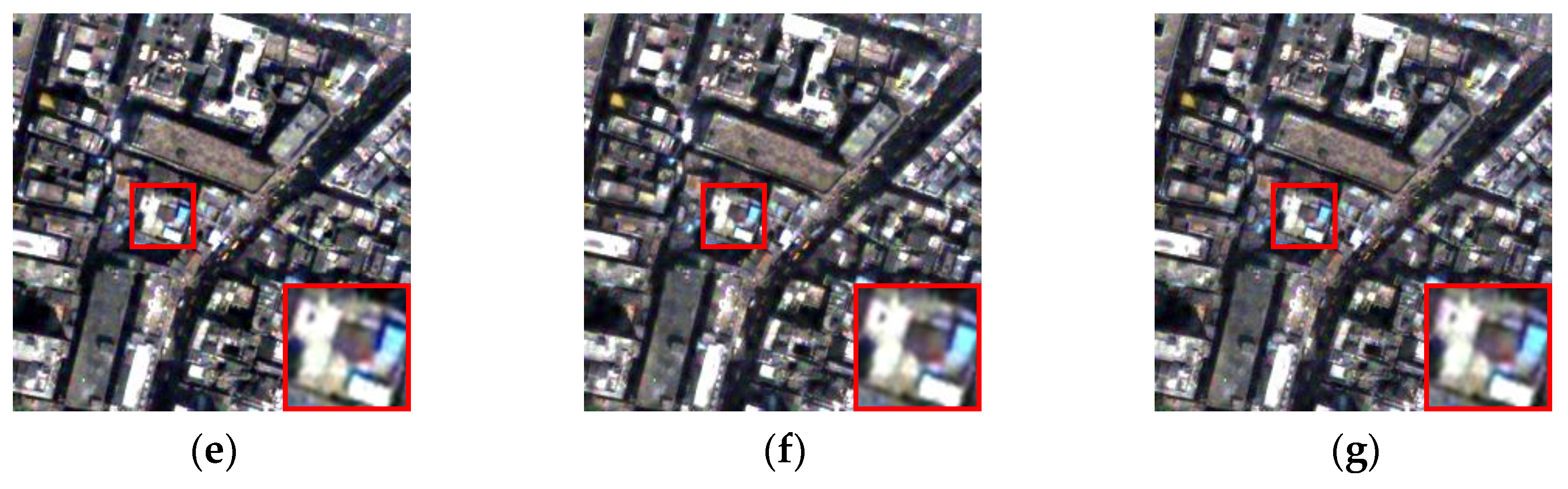
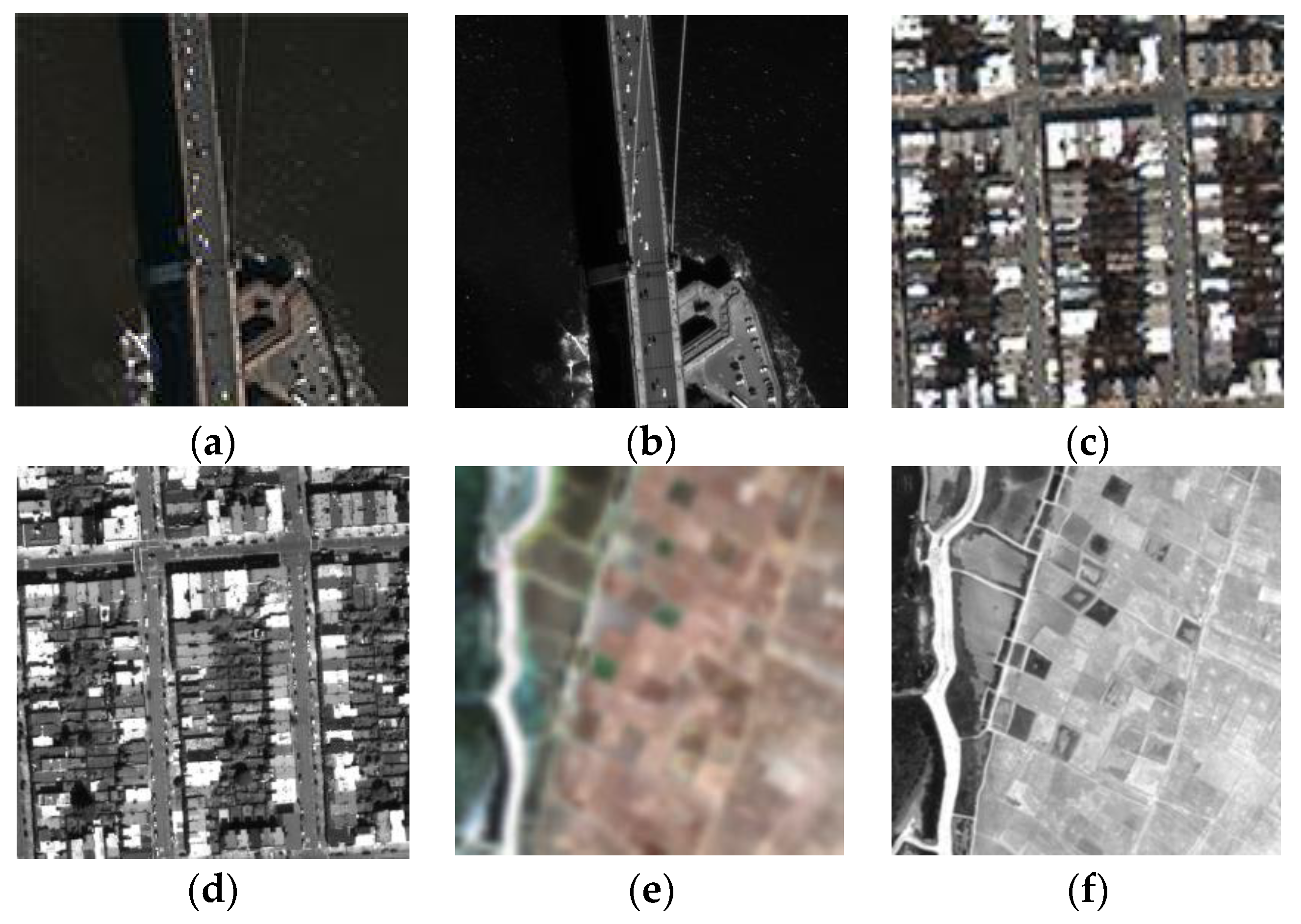
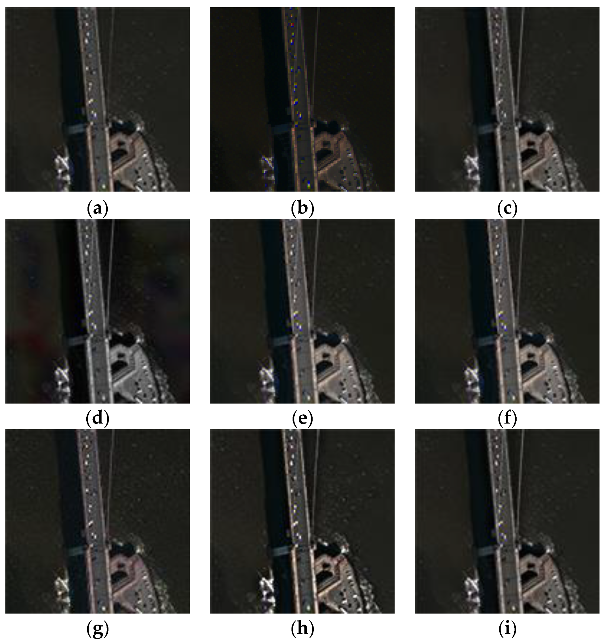
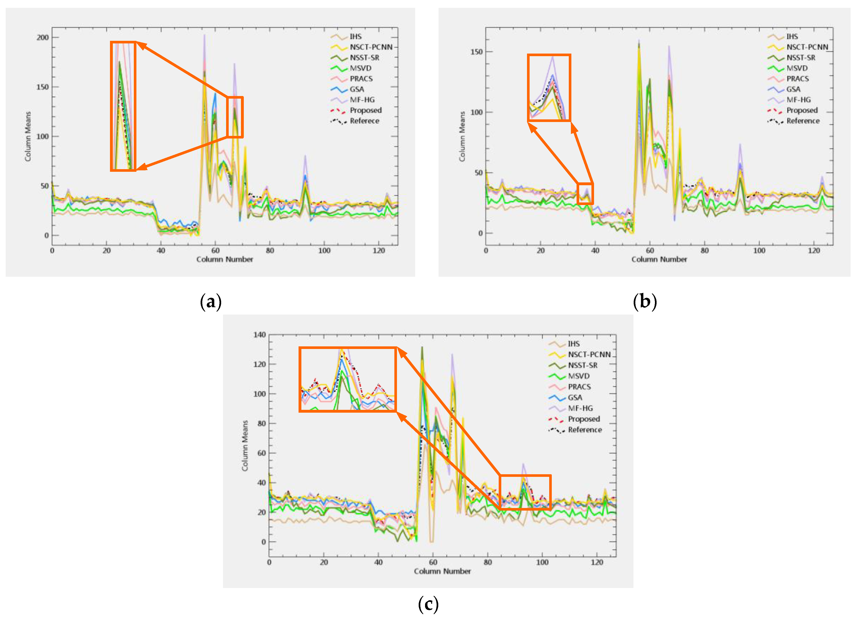
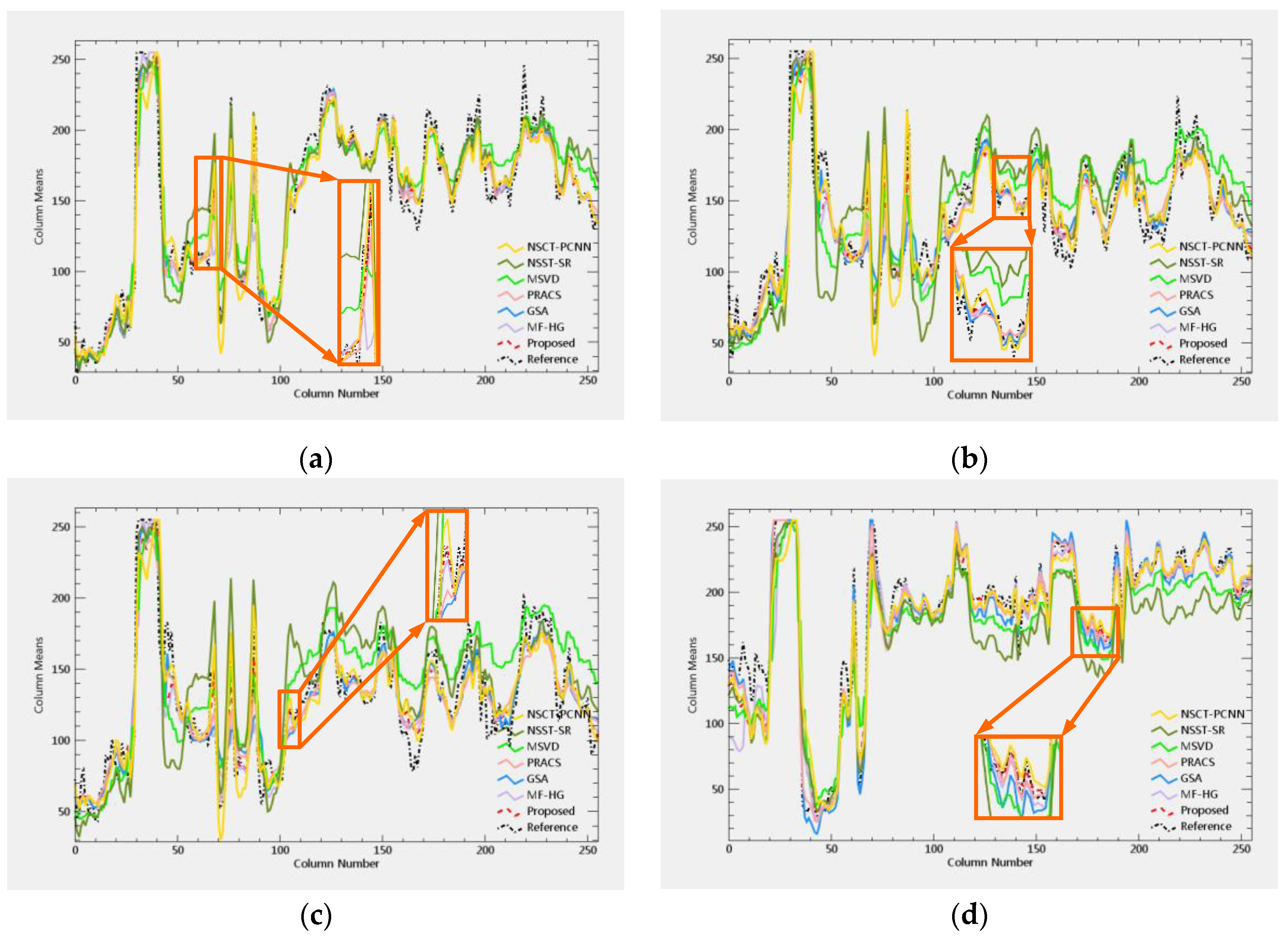
Based on a gradient domain GIF with excellent edge-preserving properties, a new fusion method of MS and PAN images in the NSST domain is proposed. The MS and PAN images are decomposed by NSST to obtain the coefficients of a different frequency. For the high-frequency coefficients in the NSST domain, an improved pulse coupled neural network (PCNN) model is used to obtain the initial firing map. Unlike previous methods that directly calculate the fusion decision map, the gradient domain GIF is used to optimize the firing map, and then the fusion decision map is calculated in order to guide the fusion of high-frequency coefficients. For the low-frequency coefficients in the NSST domain, a fusion strategy that is based on morphological filter-based intensity modulation (MFIM) technology is adopted. The gradient domain GIF is used to perform the edge refinement on the modulated low-frequency coefficients to obtain the fusion result of the low-frequency coefficients. The experimental results show that, in the proposed method, the detailed information and spatial continuity can be effectively improved while still maintaining excellent spectral information.

2. Materials and Methods

2.1. NSST

Guo and Labate [18] constructed the shearlet transform by combining geometry and multi-scale method through classical theory of the affine system. When the dimension $n=2$, the affine system is:

$$\begin{array}{ll}{\mathsf{\psi }}_{AB}(\psi )=& \{{\psi }_{j,k,l}(X)={\left|\det A\right|}^{j/2}\psi (B^l{A}^{j}X-k):\\ & j,l\in Z,k\in Z^2\}\end{array}$$

(1)

where, $\psi \in L^2({\Re }^2)$, $L$ represents the square integrable space, $A$ and $B$ are both $2\times 2$ invertible matrices, and $\left|\det B\right|=1$. If for any $f\in L^2({\Re }^2)$, ${\mathsf{\psi }}_{AB}(\psi )$ constitutes the following tight support framework, and then the element of ${\mathsf{\psi }}_{AB}(\psi )$ is called the synthetic wavelet:

$${{\displaystyle \sum _{j,k,l}{\left|\langle f,{\psi }_{j,k,l}\rangle \right|}^2=\Vert f\Vert }}^2$$

(2)

where,$A^j$ is associated with scale transformation and $B^l$ is associated with geometric transformation. In Equation (1), $A=\left[\begin{array}{ll}a& 0\\ 0& a^{1/2}\end{array}\right]$ denotes an anisotropic matrix and $B=\left[\begin{array}{ll}1& s\\ 0& 1\end{array}\right]$ denotes a shearlet matrix; at this point, the synthetic wavelet is called a shearlet and the values usually are taken as $A=A_0=\left[\begin{array}{ll}4& 0\\ 0& 2\end{array}\right]$, $B=B_0=\left[\begin{array}{ll}1& 1\\ 0& 1\end{array}\right]$. Figure 1 shows the frequency decomposition and supports of a shearlet. The frequency supported base of each element ${\widehat{\psi }}_{j,k,l}$ is a trapezoid region, the size is approximately $2^{2j}\times 2^j$, and the slope is $l{2}^{-j}$.

As the shearlet does not have a shift-invariant character, it is easy to introduce the Gibbs phenomenon in image fusion. NSST [22] is an improved form of the shearlet with directional selectivity and shift-invariance, high computational efficiency, and simple structure. NSST is mainly divided into multi-scale decomposition and multi-directional decomposition. Non-subsampled Laplacian pyramid (NSP) performs multi-scale decomposition. $J$ sub-band images of the high-frequency and one sub-band image of the low-frequency can be obtained by the $J$ level NSP decomposition, and each sub-band image has the same size as the source image. The shearlet filter (SF) implements multi-directional decomposition. ${\displaystyle \sum _{j=1}^J{2}^{l_j}+1}$ sub-band images with the same size as the source image can be obtained by the $j$ level decomposition of a certain scale. $J$ is the image decomposition layer and $l_j$ is the direction decomposition levels under scale $j$. Figure 2 illustrates a three-level NSST decomposition model. NSST has the characteristics of approximate optimal sparse representation for 2-D images. Applying it to the fusion of MS and PAN images can provide more useful information for the fused result.

2.2. Gradient Domain GIF

2.2.1. GIF

The GIF is a new kind of local linear filter. It has the edge-preserving property and its time complexity is independent of the size of filter window. It has fast calculation speed, high efficiency, and time complexity of O(n), which has been successfully applied to the field of image fusion [35]. The GIF can transfer the structural information in the guided image to the filter output, which makes the filter output more structured, so as to complete the edge correction in the fusion decision. However, the local linear model that is used in the GIF cannot represent the image well around some edges, which may result in halo artifacts. Li [33] proposed the weighted GIF, which can effectively reduce artifacts by introducing the edge-aware factors, but there is no explicit constraint to deal with edges, so in some cases the edges cannot be well preserved. Kou [34] proposed a gradient domain GIF by introducing explicit first-order edge condition constraints, so that the edges can be better preserved.

Figure 3 shows the processing flowchart of the GIF. The GIF assumes that ${\omega }_k$ is a square window whose size is $(2r_1+1)\times (2r_1+1)$ centered at a pixel $k$. $I$ is the guidance image, $Z$ is the output image, and $X$ is an image to be filtered. Equation (3) is a local linear model between the guided image and the filtered output image:

$$Z(i)=a_{k}I(i)+b_k,\forall i\in {\omega }_k$$

(3)

where, $a_k$ and $b_k$ are the linear coefficients in the window ${\omega }_k$ and have fixed values. $a_k$ and $b_k$ are calculated by minimizing the cost function $E(a_k,b_k)$, which is defined as:

$$E(a_k,b_k)={\displaystyle \sum _{i\in {\omega }_k}({(a_k{I}_i+b_k-X(i))}^2+\lambda a_k^2)}$$

(4)

where, $\lambda$ is a regularization term, which is an important parameter in adjusting the ambiguity of the filter to penalize the too-large values of $a_k$. According to linear regression analysis, the solution of Equation (4) can be obtained:

$$a_k=\frac{{\mu }_{I\odot X,r_1}(k)-{\mu }_{I,r_1}(k){\mu }_{X,r_1}(k)}{{\sigma }_{I,r_1}^2(k)+\lambda }$$

(5)

$$b_k={\mu }_{X,r_1}(k)-a_k{\mu }_{I,r_1}(k)$$

(6)

where, $\odot$ is the dot products of two matrices, ${\mu }_{I\odot X,r_1}(k)$, ${\mu }_{I,r_1}(k)$, and ${\mu }_{X,r_1}(k)$ represent the means of $I\odot X$, $I$, and $X$ in the local window ${\omega }_k$, respectively. Since the value of $\lambda$ in the GIF is fixed, the edges are inevitably smoothed, and in some cases the edges cannot be well preserved.

2.2.2. Edge-Aware Weighting

In order to better preserve the edges, Kou defines a new edge-aware weighting ${\mathsf{\Gamma }}_I(k)$, which can determine the importance of each pixel with respect to the global guidance image. ${\mathsf{\Gamma }}_I(k)$ is defined, as follows:

$${\mathsf{\Gamma }}_I(k)=\frac{1}{M}{\displaystyle \sum _{i=1}^M\frac{\chi (k)+\epsilon }{\chi (i)+\epsilon }}$$

(7)

where, $\chi (k)$ is defined as ${\sigma }_{I,1}(k){\sigma }_{I,r_1}(k)$, ${\sigma }_{I,1}(k)$, and ${\sigma }_{I,r_1}(k)$ are the variances of $I$ in window $3\times 3$ and $(2r_1+1)\times (2r_1+1)$, respectively. $r_1$ is the window size of the filter, $M$ is the pixel number in the image.

2.2.3. Gradient Domain GIF

$\nabla Z(i)=a_k\nabla I(i)$ can be obtained according to the linear model in Equation (3). Obviously, the smoothness of $Z$ in local window depends on the value of $a_k$. If the pixel $k$ is at the edge area and $a_k=1$, the edge can be preserved well. If the pixel $k$ is in a smooth region, it is expected that the $a_k=0$, so the region will be smoothed. Based on the observation, a new cost function is defined, as follows:

$$E(a_k,b_k)={\displaystyle \sum _{i\in {\omega }_k}[{(a_{k}I(i)+b_k-X(i))}^2+\frac{\lambda }{{\mathsf{\Gamma }}_I(k)}{(a_k-{\gamma }_k)}^2]}$$

(8)

where the definition of ${\gamma }_k$ is

$${\gamma }_k=1-\frac{1}{1+e^{\eta (\chi (k)-{\mu }_{\chi ,\infty })}}$$

(9)

where, ${\mu }_{\chi ,\infty }$ is the mean value of $\chi (i)$, $\eta =4/({\mu }_{\chi ,\infty }-\min (\chi (i)))$. It can be seen that, if the pixel $k$ is at the edge area, the value of ${\gamma }_k$ approaches 1. On the contrary, the value of ${\gamma }_k$ approaches 0 if the pixel is in the smooth region. The filter is less sensitive to the selection of parameter $\lambda$.

The optimal values of $a_k$ and $b_k$ are calculated, as follows

$$a_k=\frac{{\mu }_{I\odot X,r_1}(k)-{\mu }_{I,r_1}(k){\mu }_{X,r_1}(k)+\frac{\lambda }{{\mathsf{\Gamma }}_I(k)}{\gamma }_k}{{\sigma }_{I,r_1}^2(k)+\frac{\lambda }{{\mathsf{\Gamma }}_I(k)}}$$

(10)

$$b_k={\mu }_{X,r_1}(k)-a_k{\mu }_{I,r_1}(k)$$

(11)

The final value of $Z$ is:

$$Z(i)={\overline{a}}_i{I}_i+{\overline{b}}_i$$

(12)

In the calculation of the linear coefficients of the local window, a pixel may be contained in multiple windows, so $a_k$ and $b_k$ need to be calculated by mean filtering, that is:

$$Z=\frac{1}{\left|\omega \right|}{\displaystyle \sum _{k,i\in {\omega }_k}(a_{k}I(i)+b_k)={\overline{a}}_{i}I(i)+{\overline{b}}_i}$$

(13)

where ${\overline{a}}_i$ and ${\overline{b}}_i$ are the means of $a_k$ and $b_k$ in the window ${\omega }_k$, respectively. ${\overline{a}}_i=\frac{1}{\left|\omega \right|}{\displaystyle {\sum }_{k\in {\omega }_i}{a}_k}$, ${\overline{b}}_i=\frac{1}{\left|\omega \right|}{\displaystyle {\sum }_{k\in {\omega }_i}{b}_k}$, and $\left|\omega \right|$ is the number of pixels in the local window.

3. Proposed Method

The factors affecting the fusion quality of PAN and MS images mainly include two aspects: the integration of spatial details and the preservation of spectral information. The main purpose of pansharpening is to establish a good tradeoff between the injection of spatial details and the preservation of spectral information. It is assumed that PAN and MS images that are used for fusion have been geometrically registered. NSST is utilized to decompose the source images with multi-scale and multi-direction into different frequency coefficients. The high-frequency coefficients represent the detailed features of the image, which is the reflection of spatial information. The selection of high-frequency coefficients plays an important role in the maintenance of detailed spatial information and improving the spatial resolution of the fused image. The low-frequency coefficient image is the approximate version of the original image, which contains the most energy and spectral information. The selection of low-frequency coefficients is of great importance for maintaining the spectral signatures and reducing the spectral distortion of the fused result. According to the different significant features that need to be preserved in different frequency domains, the corresponding fusion rules of high- and low-frequency coefficients are proposed. Figure 4 illustrates the flowchart of the multi-scale image fusion procedure that is based on NSST, and the fusion steps are as follows:

1. NSST decomposition

The PAN and MS images are decomposed by NSST to obtain the corresponding low- and high-frequency sub-band coefficients $\{S_P^{0,d},S_P^{l,d}\}$ and $\{S_M^{0,d},S_M^{l,d}\}$. $S_P^{0,d}$ is the low-frequency coefficients of the PAN image, and $S_P^{l,d}$ is the $l$th scale, $d$th directional high-frequency coefficients of the PAN image. Similarly, $S_M^{0,d}$ and $S_M^{l,d}$ are the corresponding coefficients of the MS image.

2. Fusion of low-frequency coefficients in the NSST domain

The low frequency coefficients of the PAN and MS images are processed with fusion rule that is based on MFIM technology. The high resolution version of the low-frequency coefficients can be obtained while using low-frequency coefficients of the PAN image to modulate the low-frequency coefficients of the MS image. The gradient domain GIF is used to optimize the modulated sub-band coefficients and the fusion results of low-frequency coefficients $\{S_F^{0,d}\}$ are obtained.

3. Fusion of high-frequency coefficients in the NSST domain

The high-frequency coefficients of the PAN and MS images are processed by the improved PCNN-based fusion rule. The initial firing map is obtained by a PCNN model, the original PAN image is subsequently used as a guidance image, and then the edge preserving gradient domain GIF is performed on the firing map. According to the optimized firing map, the fusion decision map is calculated to guide the fusion of high-frequency coefficients to obtain the fusion result $\{S_F^{l,d}\}$.

4. Inverse transform of NSST

The inverse transform of NSST is performed on the fused low-frequency coefficients $\{S_F^{0,d}\}$ and the fused high-frequency coefficients $\{S_F^{l,d}\}$ to obtain the final fused image $F$.

3.1. Fusion Rule of the Low-Frequency Coefficients

The low-frequency coefficients that were decomposed by the NSST process are the inheritance of the original MS and PAN images, which are the approximate components. They contain the most energy of the original images. The fusion rule of these coefficients is designed to combine the available spatial information from the low-frequency coefficients of the PAN image and the available spectral information from the low-frequency coefficients of the MS image.

In this paper, the morphological filter-based intensity modulation (MFIM) technique [36] and gradient domain GIF based fusion rule of the low-frequency coefficients is designed. The low-frequency coefficient image serves as an approximate version of the original image, which contains the main information regarding the original image and also contains some detailed spatial information. Traditional fusion strategies for the low-frequency coefficients of the MS and PAN images usually adopt a simple weighted averaging method or the region energy analysis based method. These methods are easy to implement but they have problems in contrast reduction and detailed information loss. Furthermore, the coefficient selection or superposition procedure may result in decision bias and spectral distortion. The preservation of the spectral content of the original MS image is very important. Thus, we adopt the MFIM technique to reconstruct the spatial details that are missing in the low-frequency sub-bands of the MS image and preserve the spectral information. The gradient-domain GIF is used to refine the modulated low-frequency coefficients image in order to properly inject the coefficients of spatial details and avoid halo artifacts in the fusion results.

First, by using the low-frequency coefficients image $M{S}_k$ of the MS image as a reference image, the image histogram equalization on the low-frequency coefficient image $S_P^{0,d}$ of the PAN image is performed. In other words, the image $P_k^0$ on the band $k$ can be obtained by the equalization step between $S_P^{0,d}$ and $M{S}_k$.

The low-resolution version $P_k^{low}$ of the low-frequency coefficients image of the PAN image can be obtained by half-gradient operator that is based morphological filtering. Setting the structural element $B$ as $B=\left[\begin{array}{lll}0& 1& 0\\ 1& 1& 1\\ 0& 1& 0\end{array}\right]$, the corresponding morphological filter is as follows:

$$\begin{array}{ll}{\psi }_{\mathrm{HG},B}& =F-{\overline{\psi }}_{\mathrm{HG},B}\\ & =F-\left[0.5(F-{\epsilon }_B(F))-0.5({\delta }_B(F)-F)\right]\\ & =0.5({\epsilon }_B(F)+{\delta }_B(F))\end{array}$$

(14)

where, ${\epsilon }_B(F)$ and ${\delta }_B(F)$ are the erosion and dilation operators, respectively. $P_k^{low}$ is derived through the morphological filter and a pyramidal decomposition.

Subsequently, the spatial details can be extracted and injected. The fusion result ${\{{\widehat{MS}}_k\}}_{k=1,\dots ,N}$ can be obtained by intensity modulation of the low-frequency coefficients of the MS image ${\{{\widetilde{MS}}_k\}}_{k=1,\dots ,N}$, as follows:

$${\widehat{MS}}_k={\widetilde{MS}}_k+{\widetilde{MS}}_k\frac{P_k^0-P_k^{low}}{P_k^{low}}$$

(15)

The definition of the contrast by Weber [37] is given by $C=\Delta L/L_b$, where $\Delta L=L-L_b$, $L_b$ is the background luminance, $L$ is the pixel luminance [38], and $\Delta L$ can be seen as the foreground luminance. Equation (15) can be written as ${\widehat{MS}}_k={\widetilde{MS}}_k(1+C)$.

Finally, the gradient domain GIF is used to refine the edges in the modulated coefficients image $\widehat{MS}=\{{\widehat{MS}}_k{\}}_{k=1,\dots ,N}$. The low-frequency coefficients image of the PAN image serves as the guidance image. The final fusion result of the low-frequency coefficients can be obtained by the following equation:

$$S_F^0=GDGI{F}_{r_1,{\epsilon }_1}(\widehat{MS},S_P^{0,d})$$

(16)

3.2. Fusion Rule of the High-Frequency Coefficients

A PCNN is used to extract detailed information in the high-frequency coefficients, which is a new type of neural network with global pulse synchronization and pulsecoupling. It can realize the simultaneous firing of pixels with proximal space and similar features. The firing number of the PCNN model can effectively reflect the detailed spatial information of an image. The more time that the firing occurs, the more information that the corresponding pixel area will have in the image. The PCNN consists of several neurons, each of which consists of three parts: the receiving domain, the modulation domain, and the pulse generator. In this paper, a simplified PCNN model is adopted [39] and its expression is as follows:

$$\{\begin{array}{l}{F}_{ij}(n)=D_{ij}\\ L_{ij}(n)=L_{ij}(n-1)\times \exp (-{\alpha }_L)+V_L{\displaystyle \sum _{pq}{\omega }_{ij,pq}{Y}_{pq}(n-1)}\\ U_{ij}(n)=F_{ij}(n)(1+\beta L_{ij}(n))\\ {\theta }_{ij}(n)={\theta }_{ij}(n-1)\times \exp (-{\alpha }_{\theta })+V_{\theta }{Y}_{ij}(n-1)\\ Y_{ij}(n)=step(U_{ij}(n)-{\theta }_{ij}(n))\end{array}$$

(17)

where, $n$ denotes the iteration steps, $F_{ij}(n)$, $D_{ij}$, and $L_{ij}(n)$ are the neuron feedback input, exterior input, and linking input, respectively, the parameter $\beta$ is the connecting weight between the neurons, $U_{ij}(n)$ represents the inner activity of the neuron, ${\theta }_{ij}(n)$ is the dynamic threshold, ${\omega }_{ij,pq}$ denotes the synaptic links of the neuron, $V_L$ is the amplification factor of the linking input, $V_{\theta }$ is the threshold amplification factor, ${\alpha }_L$ and ${\alpha }_{\theta }$ denote the attenuation time constant, and $Y_{ij}(n)$ represents the PCNN output pulse of a neuron. If $U_{ij}(n)>{\theta }_{ij}(n)$, then the neuron generates a pulse value $Y_{ij}(n)=1$, called a single firing. After $n$ iterations, the firing map that is generated by the total numbers of firings of each neuron becomes the PCNN model output.

Based on the simplified PCNN model, a soft limited amplitude sigmoid function is used to calculate the firing output amplitude of the model during the iterative process:

$$T_{ij}(n)=\frac{1}{1+e^{{\theta }_{ij}(n)-U_{ij}(n)}}$$

(18)

After $n$ iterations of the PCNN, the sum of the firing output amplitude is:

$$Z_{ij}(n)=Z_{ij}(n-1)+T_{ij}(n)$$

(19)

The gradient domain GIF is used to optimize the firing map that is exported by the PCNN model, which aims to satisfy the spatial consistency and therefore reduce the artificial texture and image non-uniformity produced by the multi-scale fusion methods. $W^P$ and $W^M$ denote the firing maps of the PAN and MS images that were optimized by gradient domain GIF, respectively:

$$W^P=GDGI{F}_{r_2,{\epsilon }_2}(Z^P,I^M), W^M=GDGI{F}_{r_2,{\epsilon }_2}(Z^M,I^M)$$

(20)

Based on observation, the fusion decision matrix can be obtained as:

$$H(i,j)=\{\begin{array}{l}1, W_{ij}^M(N_{\max })>W_{ij}^P(N_{\max })\\ 0, \mathrm{else}\end{array}$$

(21)

The fusion result of the high-frequency coefficients can then be calculated according to the decision matrix:

$$S_F(i,j)=S_M(i,j)H(i,j)+S_P(i,j)\left[1-H(i,j)\right]$$

(22)

where, $S_M(i,j)$ and $S_P(i,j)$ represent the high-frequency coefficients of the MS and PAN images, respectively.

4. Result

4.1. Data Set

In our experiment, the data sets that were acquired by WorldView-2 and QuickBird satellites are used to evaluate the proposed fusion method. The main features of these two satellites are given in

Table 1. The spectral and spatial resolution of each band of the WorldView-2 satellite.

Spectral Bands	Wavelength Range (nm)	Spatial Resolution (m)	Comment
Band 1	400–450	1.84	Coastal Blue
Band 2	450–510		Blue
Band 3	510–580		Green
Band 4	585–625		Yellow
Band 5	630–690		Red
Band 6	705–745		Red Edge
Band 7	770–895		Near-Infrared 1
Band 8	860–1040		Near-Infrared 2
Panchromatic wave band	450–800	0.46

and

Table 2. The spectral and spatial resolution of each band of the QuickBird satellite.

Spectral Bands	Wavelength Range (nm)	Spatial Resolution (m)	Comment
Band 1	450–520	2.88	Blue
Band 2	520–600		Green
Band 3	630–690		Red
Band 4	760–900		Near-Infrared
Panchromatic wave band	450–900	0.72

. The MS and PAN images that were used in the experiment have been registered. The WorldView-2 data set was collected by the Beijing Key Laboratory of Digital Media. The sizes of the PAN and MS images are 512×512 and 128×128, respectively. Eight multi-spectral wave bands, including four standard bands and four new bands are contained in the WorldView-2 satellite, but the data set only provides three bands of 5 (R), 3 (G), and 2 (B) for the MS image. The land-cover types of the MS and PAN images include home, seaside, urban, house, and bridge. Given space limitations, four pairs of MS and PAN images are considered for the comparison analysis of our proposed method, two performed at reduced resolution and two evaluated at the original resolution. The second data set was captured by the QuickBird satellite on November 21, 2002, which covers the national forest park of Sundarbans, India. The sizes of the PAN and MS images are 256×256 and 64×64, respectively. This data set provides the MS image with four bands (R, G, B, and NIR). Two pairs of MS and PAN images are selected for the result analysis as an example, one for full resolution assessment and the other for reduced resolution assessment.

4.2. Quality Assessment of Fusion Results

Generally, the quality assessment of an image fusion method includes subjective and objective evaluations. Subjective evaluation that is based on individuals may have differences, meaning that the assessment faces a challenge of reliability, so an objective evaluation is needed to provide a complementary and quantitative evaluation system.

Because of the absence of reference images, two strategies have been proposed in order to measure the fusion quality. One is evaluated on the degraded images that are based on Wald’s protocol; the other is performed on the full resolution without the reference images. For the degraded evaluation, the original MS and PAN images are processed by a low-pass filter with a down-sampling factor of four to obtain the reduced resolution images, and the original MS image is taken as the reference image. The other strategy calculates quality indices by operating on the relationship between the original MS and PAN images and the fused images.

As detailed below, nine well-known indices are utilized to evaluate the spatial and spectral qualities of the fused results. The correlation coefficient ($\mathrm{CC}$) reflects the similarity of spectral features, and structural similarity ($\mathrm{SSIM}$) is a structural similarity index. The spectral angle mapper ($\mathrm{SAM}$) is utilized to measure the spectral distortion. Root mean square error ($\mathrm{RMSE}$), erreur relative global adimensionnelle de synthèse ($\mathrm{ERGAS}$), and the universal image quality index ($\mathrm{UIQI}$) measures the global quality of spectral and spatial features. The “quality with no reference” ($\mathrm{QNR}$) indicator measures the overall quality of the fused image and it is composed of two separate indices, the spatial distortion index $D_s$ and the spectral distortion index $D_{\lambda }$.

4.2.1. Reduced-Resolution Assessment

Follow Wald’s protocol, the reduced resolution assessment is based on the scale invariance assumption. Six indices have been selected for the evaluation procedure, which consider the available reference images. The indices are described, as follows:

1. Correlation Coefficient ($\mathrm{CC}$)

$\mathrm{CC}$ [40] indicates the presentation ability of the spectral characteristics. It reflects the correlation degree of spectral features between each band of the fusion MS image and the reference image, and the ideal value is 1. The definition is as follows:

$$C{C}_k=\frac{{\displaystyle \sum _{m=1}^M{\displaystyle \sum _{n=1}^N\left[(F_k(m,n)-{\overline{F}}_k)\times (R_k(m,n)-{\overline{R}}_k)\right]}}}{\sqrt{{\displaystyle \sum _{m=1}^M{\displaystyle \sum _{n=1}^N{(F_k(m,n)-{\overline{F}}_k)}^2\times }}{\displaystyle \sum _{m=1}^M{\displaystyle \sum _{n=1}^N{(R_k(m,n)-{\overline{R}}_k)}^2}}}}$$

(23)

where, $C{C}_k$ is the correlation coefficient of the band $k$, ${\overline{F}}_k$, and ${\overline{R}}_k$ denote pixel means of the $k$ band of the fusion MS image and the reference image, respectively.

2. Structural Similarity ($\mathrm{SSIM}$)

$\mathrm{SSIM}$ [41] reflects the structural similarity between the fused image and the reference image. It quantifies the degradation of image quality. A higher value of $\mathrm{SSIM}$ indicates a higher structural similarity between the two images.

$$SSIM(R,F)=\frac{(2{\mu }_R{\mu }_F+C_1)(2{\sigma }_{RF}+C_2)}{({\mu }_R^2+{\mu }_F^2+C_1)({\sigma }_R^2+{\sigma }_F^2+C_2)}$$

(24)

where ${\mu }_R$ and ${\mu }_F$ denote the mean values of the reference image $R$ and the fused image $F$, respectively. ${\sigma }_R$ and ${\sigma }_F$ are the variances of $R$ and $F$. ${\sigma }_{RF}$ calculates the covariance value of $R$ and $F$. $C_1$ and $C_2$ are constants, which exist to avoid the denominator equaling to 0 and to maintain stability. In order to simplify the model, the value is set to 0.

3. Spectral Angle Mapper ($\mathrm{SAM}$)

A simple index, $\mathrm{SAM}$ [42], reflects the distortion in spectral information between the fused MS image and the reference image, and the ideal value is 0. Its definition is as follows:

$$SAM=\arccos \left[\frac{\langle u_R,u_F\rangle }{{\Vert u_R\Vert }_2{\Vert u_F\Vert }_2}\right]$$

(25)

where $u_F$ and $u_R$ are the spectral vectors constructed by the fused image and the reference image.

4. Root Mean Square Error ($\mathrm{RMSE}$)

$\mathrm{RMSE}$ [43] is the index accounts for the difference between the reference image and the fused image; the ideal value is 0. $\mathrm{RMSE}$ is defined as

$$RMSE=\sqrt{\frac{1}{MN}{\displaystyle \sum _{m=1}^M{\displaystyle \sum _{n=1}^N{(F(m,n)-R(m,n))}^2}}}$$

(26)

5. Erreur Relative Global Adimensionnelle de Synthèse ($\mathrm{ERGAS}$)

ERGAS [13] reflects the distortion degree of the spectral and spatial information, and it is an index for the overall evaluation of the fused image. The optimal value of ERGAS is 0. The definition is as follows:

$$ERGAS=100\frac{h}{l}\sqrt{\frac{1}{N}{{\displaystyle \sum _{k=1}^N\left[\frac{RMS{E}_k}{Mean(R_k)}\right]}}^2}$$

(27)

where $h$ and $l$ are the spatial resolution of the PAN and MS images, respectively. ${\mathrm{RMSE}}_k$ is the mean square error between the $k$ band of the fused image and the $k$ band of the reference image, indicating the difference between the two images, and $\mathrm{Mean}(R_k)$ denotes the mean value of the band $k$ of the reference image.

6. Universal Image Quality Index ($\mathrm{UIQI}$)

$\mathrm{UIQI}$ [44] is a performance index that measures the spatial details of the fused MS images. The optimal value is 1; so the closer that UIQI value is to 1, the better the fusion quality. It is defined as:

$$UIQI(R,F)=\frac{{\sigma }_{RF}}{{\sigma }_R{\sigma }_F}\times \frac{2\overline{FR}}{{\overline{F}}^2+{\overline{R}}^2}\times \frac{2{\sigma }_R{\sigma }_F}{{\sigma }_R^2+{\sigma }_F^2}$$

(28)

where, ${\sigma }_R$ and ${\sigma }_F$ are the standard deviations of the reference image $R$ and the fused image $F$, respectively. ${\sigma }_{RF}$ calculates the covariance value of $R$ and $F$.

4.2.2. Full-Resolution Assessment

In order to operate the assessment directly on the data at the original resolution, the quality with no reference ($\mathrm{QNR}$) index was proposed [45]. This index measures the correlation, luminance, and contrast between the two images. $\mathrm{QNR}$ is composed of two separate indices,$D_{\lambda }$ and $D_s$, which denote the distortion of spectral and spatial features, respectively.

1. Quality with No Reference (QNR)

QNR, which consists of $D_{\lambda }$ and $D_s$, reflects the overall quality of the fused image, and the ideal value is 1. The definition of $\mathit{QNR}$ is as follows:

$$QNR=(1-D_{\lambda })\cdot (1-D_s)$$

(29)

2. Spectral Distortion Index ($D_{\lambda }$)

$D_{\lambda }$ represents the spectral distortion degree between the fused image and the MS image, with an ideal value of 0. The definition of $D_{\lambda }$ is as follows:

$$D_{\lambda }={}^p\sqrt{\frac{1}{N(N-1)}{\displaystyle \sum _{i=1}^N{\displaystyle \sum _{j=1,i\ne j}^N{\left|UIQI(M{S}_i,M{S}_j)-UIQI(F_i,F_j)\right|}^p}}}$$

(30)

where, $p$ is the difference enhancement parameter that isusually set to 1, $UIQI(M{S}_i,M{S}_j)$ and $UIQI(F_i,F_j)$ are the generalized image quality indicators of the MS image bands and the fused image bands, respectively; $UIQI(M{S}_i,M{S}_j)=\frac{{\sigma }_{M{S}_{i}M{S}_j}}{{\sigma }_{M{S}_i}\cdot {\sigma }_{M{S}_j}}\times \frac{2\overline{M{S}_i}\cdot \overline{M{S}_j}}{{\overline{M{S}_i}}^2+{\overline{M{S}_j}}^2}\times \frac{2{\sigma }_{M{S}_i}\cdot {\sigma }_{M{S}_j}}{{\sigma }_{M{S}_i}^2+{\sigma }_{M{S}_j}^2}$, where ${\sigma }_{M{S}_{i}M{S}_j}$ is the image covariance, ${\sigma }_{M{S}_i}$ and ${\sigma }_{M{S}_j}$ represent image variances, and $\overline{M{S}_i}$ and $\overline{M{S}_j}$ denote the image mean values.

3. Spatial Distortion Index ($D_s$)

$D_s$ indicates the information preservation of the fused image in the spatial domain, with an ideal value of 0. Its definition is as follows:

$$D_s={}^q\sqrt{\frac{1}{N}{\displaystyle \sum _{i=1}^N{\left|UIQI(M{S}_i,PAN)-UIQI(F_i,PAN)\right|}^q}}$$

(31)

where, $q$ is the difference enhancement parameter that is usually set to 1, $UIQI(M{S}_i,PAN)$ is the generalized image quality indicator between the $k$ band of the MS image and the PAN image, and $UIQI(F_i,PAN)$ is the generalized image quality indicator between the $k$ band of the fused image and the PAN image.

4.3. Implementation Details

The implementation details for the fusion methods are provided and analyzed. The experimental hardware environment is an Intel Core i5-4200U, 1.60GHz CPU, and 4GB memory. The software environment is MATLAB R2014a. The parameters of the fusion methods are set, as follows: the NSST decomposition filter is “maxflat”, the scale decomposition layer is set to 3, and the corresponding directions to $\{16,8,4\}$. In the PCNN model, $n=200$, ${\alpha }_L=1.0$, ${\alpha }_{\theta }=0.2$, $\beta =3.0$, $V_L=1.0$, and $V_{\theta }=20$. The two parameters $r$ and $\epsilon$ of the gradient domain GIF affect the fusion performance of the proposed method to some extent. The parameter $r$ is the size of the filter window, which determines the significant difference of the guidance image in local windows. $\epsilon$ denotes the normalized parameter, which determines the blur degree of guided filter.

The effects of the two sets of parameters, $r_1$, ${\epsilon }_1$ and $r_2$, ${\epsilon }_2$, in the gradient domain GIF on fusion performance will be discussed. Four indices, $\mathrm{CC}$, $\mathrm{SAM}$, $\mathrm{ERGAS}$, and $\mathrm{UIQI}$, are adopted to analyze the performance impact of the four parameters. Figure 5a,b,d,e represent two groups of the MS and PAN images from the WorldView-2 data set, which are the plant and house areas, respectively. Figure 5c,f is the fusion results that were obtained with the optimal guided filter parameters.

When the parameter $r_1$ is analyzed, the other three parameters are set to fixed values: ${\epsilon }_1=1$, $r_2=3$, and ${\epsilon }_2={10}^{-6}$.

Table 3. The performance evaluation results with different window sizes $r_1\times r_1$.

Image	Quality Indices	Ideal Value	${\mathit{r}}_1\times {\mathit{r}}_1$
			2 × 2	3 × 3	5 × 5	7 × 7	9 × 9	11 × 11
plant	CC	1	0.8814	0.8757	0.8602	0.8428	0.8268	0.8125
	SAM	0	8.4743	8.7137	9.2287	9.7403	10.1828	10.5024
	ERGAS	0	8.7972	8.8649	9.1230	9.4468	9.7414	9.9903
	UIQI	1	0.7340	0.7289	0.7135	0.6973	0.68465	0.6747
house	CC	1	0.9624	0.9592	0.9495	0.9398	0.9332	0.9287
	SAM	0	8.5585	8.7392	8.9066	8.9936	9.0034	8.9866
	ERGAS	0	5.6564	5.7673	6.2312	6.7068	7.0225	7.2251
	UIQI	1	0.9512	0.9482	0.9374	0.9266	0.9191	0.9138

shows the results of the fusion performance on the two pairs of test images, in terms of four selected indices ($\mathrm{CC}$, $\mathrm{SAM}$, $\mathrm{ERGAS}$, and $\mathrm{UIQI}$) versus different window sizes $r_1$. Figure 6 shows the change trend of each index intuitively, in which the indices $\mathrm{SAM}$ and $\mathrm{ERGAS}$ have been normalized. It can be seen that the performance is optimal when $r_1=2$.

When analyzing the parameter ${\epsilon }_1$, the other three parameters are also set to fixed values: $r_1=2$, $r_2=3$, and ${\epsilon }_2={10}^{-6}$. As shown in

Table 4. The performance evaluation results with different values of ${\epsilon }_1$.

Image	Quality Indices	Ideal Value	${\mathit{\epsilon }}_1$
			1	0.3	0.2	0.1	${10}^{-3}$	${10}^{-6}$
plant	CC	1	0.8814	0.8815	0.8815	0.8816	0.8835	0.8854
	SAM	0	8.4743	8.4624	8.4628	8.4483	8.3527	8.3177
	ERGAS	0	8.7972	8.7970	8.7968	8.7969	8.7830	8.7869
	UIQI	1	0.7340	0.7340	0.7341	0.7341	0.7356	0.7370
house	CC	1	0.9624	0.9624	0.9624	0.9625	0.9633	0.9636
	SAM	0	8.5585	8.5721	8.5616	8.5714	8.5129	8.4953
	ERGAS	0	5.6564	5.6582	5.6594	5.6617	5.6915	5.7057
	UIQI	1	0.9512	0.9512	0.9512	0.9512	0.9514	0.9515

, statistics of all evaluation indices of fusion images that were obtained by different values of ${\epsilon }_1$ are presented. Figure 7 shows the relevant changing curve of each index; as can be seen, better performance results came from setting the parameter ${\epsilon }_1={10}^{-6}$.

When the parameter $r_2$ is analyzed, the other three parameters are set to: $r_1=2$, ${\epsilon }_1={10}^{-6}$, and ${\epsilon }_2={10}^{-6}$, respectively. The statistical results of each evaluation index that are obtained by different window sizes $r_2\times r_2$ are presented in

Table 5. The performance evaluation results with different window sizes $r_2\times r_2$.

Image	Quality Indices	Ideal Value	${\mathit{r}}_2\times {\mathit{r}}_2$
			2 × 2	3 × 3	5 × 5	7 × 7	9 × 9	11 × 11
plant	CC	1	0.8879	0.8854	0.8815	0.8794	0.8774	0.8758
	SAM	0	8.1915	8.3177	8.4378	8.5332	8.5715	8.5824
	ERGAS	0	8.7320	8.7869	8.8861	8.9400	8.9871	9.0244
	UIQI	1	0.7414	0.7370	0.7314	0.7281	0.7258	0.7241
house	CC	1	0.9642	0.9636	0.9627	0.9618	0.9609	0.9601
	SAM	0	8.3216	8.4953	8.7911	9.0215	9.3564	9.4627
	ERGAS	0	5.7053	5.7057	5.7105	5.7368	5.7735	5.8002
	UIQI	1	0.9520	0.9515	0.9503	0.9492	0.9482	0.9476

. Figure 8 shows the change curve of each evaluation index and it can be seen that the performance is optimal when $r_2=2$.

When analyzing the parameter ${\epsilon }_2$, the other three parameters are also set to fixed values: $r_1=2$, ${\epsilon }_1={10}^{-6}$, and $r_2=2$, respectively. As shown in

Table 6. The performance evaluation results with different values of ${\epsilon }_2$.

Image	Quality Indices	Ideal Value	${\mathit{\epsilon }}_2$
			1	0.3	0.2	0.1	${10}^{-3}$	${10}^{-6}$
plant	CC	1	0.8861	0.8863	0.8864	0.8865	0.8876	0.8879
	SAM	0	8.2243	8.2472	8.2317	8.2434	8.2069	8.1915
	ERGAS	0	8.7729	8.7724	8.7684	8.7721	8.7404	8.732
	UIQI	1	0.7382	0.7383	0.7385	0.7387	0.7408	0.7414
house	CC	1	0.9638	0.9638	0.9638	0.9639	0.9642	0.9642
	SAM	0	8.4131	8.4016	8.3662	8.3470	8.3023	8.3216
	ERGAS	0	5.7100	5.7134	5.7151	5.7170	5.7068	5.7053
	UIQI	1	0.9516	0.9516	0.9516	0.9516	0.9520	0.9520

, the performance results with different values of ${\epsilon }_2$ for the proposed and other comparison methods are presented. Figure 9 shows the relevant changing curve of each index and the best performance results came from setting the parameter ${\epsilon }_1={10}^{-6}$.

By analyzing the performance with different parameter settings in the gradient domain GIF for the proposed method on WorldView-2 data set, we find that the proposed method achieves better results when the four parameters are set as $r_1=2$, ${\epsilon }_1={10}^{-6}$, $r_2=2$, and ${\epsilon }_2={10}^{-6}$. At the same time, it can be observed that the gradient domain GIF is less sensitive to the selection of the blur degree parameter. From our experiment, the performance with the no-reference indices for the proposed method also achieves the best results under the same parameter settings. The proposed method is independent of the precise parameter selection of the gradient domain GIF. These parameters of the filter have little effect on the overall fusion performance. Therefore, a satisfactory effect can be obtained by the proposed method with fixed parameter values.

4.4. Results Analysis and Discussion

In this section, the experiments are performed on the real data and the degraded data, respectively. Six image pairs of the experimental data set are from different observation scenes of the WorldView-2 and QuickBird satellites: three groups are used as the real data and the other three are applied to the performance comparison on the degraded data.

4.4.1. Performance Comparison with State-of-the-Art methods on Real Data

In this experiment, the proposed fusion method is compared with IHS [1], NSCT-PCNN [20], NSST-SR [23], multi-resolution singular value decomposition (MSVD) [46], PRACS [6], Gram–Schmidt adaptive (GSA) [7], and morphological filter-half gradients (MF-HG) [36] on the real remote sensing data set without a reference image. The codes for the seven comparison methods were downloaded from the homepage that was published by the authors and the parameter settings in the experiment are consistent with those in the literature. As shown in Figure 10, three image pairs of experimental data sets are selected as examples for the result analysis without a reference image. The first two image pairs came from two different observation scenes of the WorldView-2 satellite and the third one was collected from the QuickBird satellite. Figure 11, Figure 12 and Figure 13 show the fusion results of the proposed method and the comparison methods. For better comparison, a rectangular sub-image area is magnified and then displayed at the upper left of the fusion image.

1. WorldView-2 Data Set

For the group 1 image pair of the WorldView-2 data set, the corresponding fused products are given in Figure 11a–h. The fusion results of IHS, NSCT-PCNN, NSST-SR, MSVD, PRACS, GSA, and MF-HG are shown in Figure 11a–g, respectively; Figure 11h is the result that is generated by our method. It can be seen that the fused image that was obtained by the proposed method achieves a satisfactory visual effect in terms of the preservation of spectral information and spatial details. When compared with the other methods, there is a severe spectral distortion in the fused image that is obtained by the IHS method. The spatial and spectral quality of fusion result of the NSCT-PCNN method is relatively good. The fused result of NSST-SR suffers from some degrees of color distortion, and from the enlarged rectangle sub-image we can see that there are not enough details of the cars. The fusion results of the MSVD and GSA methods have some blurring at the edges of the cars. The PRACS method results in some noise in the dark area next to the cars. The MF-HG method shows the quality of the spectral information preservation and the spatial details injection is enhanced.

For the group 2 image pair of the WorldView-2 data set, Figure 12 shows the corresponding experimental results. By comparing the visual effects with the other comparison methods, we can find that the proposed method has significant improvement on the spatial quality and the spectral fidelity of the fused image. Figure 12a shows the fused image of the IHS method. It can be seen that this method generates serious spectral distortion. The NSCT-PCNN method injects more spatial details and it preserves more spectral information than the IHS method. The NSST-SR method has higher spatial resolution, but the color of the fusion result is quite different from the original MS image, and there is a certain degree of spectral distortion. The fusion result of the MSVD has little blurring. The PRACS, GSA, and MF-HG methods result in better spectral information maintenance, as well as improved spatial quality. It is difficult to tell the difference between the results that were obtained by these methods through visual observation.

Table 7. Objective evaluation of the experimental results shown in Figure 11.

Quality Indices	Pansharpening Algorithms
	IHS	NSCT-PCNN	NSST-SR	MSVD	PRACS	GSA	MF-HG	Proposed
$D_{\lambda }$	0.1204	0.0441	0.0092	0.0376	0.0217	0.0272	0.0087	0.0242
$D_s$	0.1541	0.0458	0.0378	0.0526	0.0436	0.0315	0.0399	0.0147
QNR	0.7440	0.9121	0.9533	0.9118	0.9356	0.9422	0.9517	0.9615

and

Table 8. Objective evaluation of the experimental results shown in Figure 12.

Quality Indices	Pansharpening Algorithms
	IHS	NSCT-PCNN	NSST-SR	MSVD	PRACS	GSA	MF-HG	Proposed
$D_{\lambda }$	0.1446	0.0479	0.0501	0.0369	0.0806	0.0679	0.0415	0.0282
$D_s$	0.1028	0.0868	0.1789	0.0524	0.0516	0.0252	0.0366	0.0456
QNR	0.7675	0.8695	0.7799	0.9126	0.8719	0.9086	0.9234	0.9274

provide the quantitative evaluation results of Figure 11 and Figure 12. From the comparison of each index, we can see that the proposed method provides the best value in terms of $\mathrm{QNR}$. In Table 7, the $D_s$ value of our proposed method is the smallest, but the MF-HG method gives the best value of $D_{\lambda }$. In Table 8, our proposed method provides the best value of $D_{\lambda }$, and the best value of $D_s$ is given by the GSA method; the result of our method is the third smallest. In general, however, the proposed method achieves better pansharpening performance than the comparison methods.

2. QuickBird Data Set

For the group 3 image pair in Figure 10e,f, which came from the QuickBird satellite, the corresponding fusion products are shown in Figure 13. The IHS method has certain limitations; namely, it can only be applied to the MS image with three bands. This data set from the QuickBird satellite provides the MS image with four bands (R, G, B, and NIR), so the methods other than IHS are used for comparison. When compared with the visual effects of the fusion results, there is a relatively serious spectral and spatial distortion in the results that were achieved by the NSCT-PCNN and NSST-SR methods. The fusion result of the MSVD method suffers from some blurring and it has an obviously serrated border. The fusion result of the GSA method has some improvement in terms of the spatial and spectral quality, but spectral inhomogeneity exists in local areas. The PRACS, MF-HG, and our proposed methods obtain better visual effects, which have higher spatial quality and better spectral information maintenance ability.

Table 9. Objective evaluation of the experimental results shown in Figure 13.

Quality Indices	Pansharpening Algorithms
	NSCT-PCNN	NSST-SR	MSVD	PRACS	GSA	MF-HG	Proposed
$D_{\lambda }$	0.0833	0.1263	0.1065	0.0044	0.0325	0.0270	0,0168
$D_s$	0.0866	0.1005	0.0171	0.0317	0.0634	0.0242	0.0161
QNR	0.8373	0.7859	0.8782	0.9640	0.9061	0.9494	0.9674

shows the corresponding quantitative results of Figure 13, in which we can see that the proposed method outperforms the six compared methods in the $\mathrm{QNR}$ and $D_s$ indices, while the best value of $D_{\lambda }$ is given by the PRACS method.

4.4.2. Performance Comparison with State-of-the-Art Methods on Degraded Data

In this experiment, the performance of the proposed fusion method is compared with seven state-of-the-art methods, including IHS [1], NSCT-PCNN [20], NSST-SR [23], MSVD [46], PRACS [6], GSA [7], and MF-HG [36], on the degraded remote sensing data set with the reference image. As shown in Figure 14, three image pairs are selected for the reduced resolution evaluation. The first two image pairs came from two different observation scenes of the WorldView-2 satellite and the third was collected from the QuickBird satellite. The low resolution images can be generated by modulation transfer functions (MTF) filtering and decimation. The original MS images are used as the reference images for performance evaluation. Figure 15, Figure 17, and Figure 19 show the fusion results of the proposed method and the compared methods.

1. WorldView-2 Data Set

For the group 1 image set, which is the degraded data set of WorldView-2 on the bridge area, the corresponding fused results are shown in Figure 15. Figure 15a is the reference MS image. Figure 15b–i demonstrate the fusion results of IHS, NSCT-PCNN, NSST-SR, MSVD, PRACS, GSA, MF-HG, and our proposed method, respectively. It can be seen that serious spectral distortion is produced by the IHS method. The fusion result of the NSCT-PCNN method behaves relatively well in terms of spectral maintenance and spatial information injection. The spatial detailed information in the fused result of NSST-SR is well maintained, but there are some color distortions. The fusion results of the MSVD and PRACS also behave well in terms of spectral and spatial information. From Figure 15g, we can see that some detailed information is lost in the result of the GSA method, with some blurring of the outlines of the bridge. In the fusion result that was obtained by the MF-HG method, the contrast in local areas is slightly higher than that in the reference image. By contrast, the fusion image of the proposed method is closer to the reference image, and it has higher spatial resolution than the comparison methods.

For better analysis of the spectral preservation ability of the fused images in Figure 15, the horizontal profiles of the column means for R, G, and B bands of the fusion images that were obtained by different methods are displayed in Figure 16. The profile that was formed by black dots is the reference image. The closer to this dotted profile, the better the spectral characteristics are preserved. It can be seen that the profile of the IHS method has large deviations from the reference images in most areas. In contrast, the fused image that was obtained by the proposed method is most similar to the horizontal spectral profile of the reference image, and it has the highest fidelity for the spectral information.

Group 2 image pair in Figure 14 is the degraded data set of WorldView-2 on the urban area, and Figure 17 shows the corresponding fusion results of the compared methods and the proposed method. Figure 17a is the original MS image, which is used as the reference image for evaluation. There is serious spectral distortion in the fused result that was obtained by the IHS method. The color of the fusion result of the NSST-SR method has a certain degree of spectral distortion. The fusion result that was obtained by the MSVD method is blurred. Fusion results yielded by the NSCT-PCNN, PRACS, GSA, MF-HG, and our proposed methods achieve better visual effects and have a more similar appearance to the reference MS image.

Figure 18 shows the horizontal spectral profiles of the fused images on urban area. It can be seen that the IHS profile has a large degree of deviation from the reference image. The horizontal profiles of NSCT-PCNN, NSST-SR, GSA, and MF-HG methods are close to the reference image, with only some local sections having differences. The horizontal spectral profile of the proposed method is closest to the reference image.

In this experiment, six indices are selected for the evaluation procedure on the degraded data, including $\mathrm{CC}$, $\mathrm{SSIM}$, $\mathrm{SAM}$, $\mathrm{RMSE}$, $\mathrm{ERGAS}$, and $\mathrm{UIQI}$. From

Table 10. Objective evaluation of the experimental results shown in Figure 15.

Quality Indices	Pansharpening Algorithms
	IHS	NSCT-PCNN	NSST-SR	MSVD	PRACS	GSA	MF-HG	Proposed
CC	0.9439	0.9556	0.9551	0.9705	0.9680	0.9625	0.9704	0.9728
SSIM	0.7698	0.9094	0.8777	0.9114	0.9473	0.8975	0.9315	0.9496
SAM	4.1703	3.8173	6.6869	2.5209	2.7412	2.0694	0.4814	2.3857
RMSE	21.1458	8.2419	12.207	10.1403	10.1918	7.403	10.8719	6.9643
ERGAS	22.6936	5.2036	8.4600	7.2728	6.1008	4.7421	6.6695	4.3979
UIQI	0.6869	0.8768	0.8011	0.9046	0.9201	0.8587	0.9118	0.9368

and

Table 11. Objective evaluation of the experimental results shown in Figure 17.

Quality Indices	Pansharpening Algorithms
	IHS	NSCT-PCNN	NSST-SR	MSVD	PRACS	GSA	MF-HG	Proposed
CC	0.9624	0.9721	0.9853	0.9436	0.9846	0.9788	0.9829	0.9883
SSIM	0.7101	0.9070	0.9469	0.8622	0.9450	0.9256	0.9238	0.9503
SAM	4.1115	5.5144	4.3565	7.46	0.5834	3.7241	0.8090	4.3772
RMSE	51.8986	15.2865	12.5691	22.5601	15.9296	15.9367	17.8641	10.626
ERGAS	22.4190	3.8395	2.9938	5.3072	3.9597	3.9836	4.7371	2.6909
UIQI	0.7255	0.9697	0.9836	0.9369	0.9734	0.9718	0.9674	0.9868

we can see that the largest $\mathrm{CC}$ values are achieved by the proposed method, which are significantly higher than other methods, indicating that our method has excellent spectral preservation ability. The proposed method also obtains the best values in $\mathrm{RMSE}$, $\mathrm{ERGAS}$ and $\mathrm{SSIM}$. It demonstrates that the fused image that was obtained by our method maintains good spatial information and has the most similar structure to the reference image. The optimal value of the $\mathrm{UIQI}$ index shows that the spatial details preservation of the proposed method is the best. The value of $\mathrm{SAM}$ is close to the optimal value of the compared methods. According to the subjective visual effect and objective evaluation using the WorldView-2 data set, the proposed method not only improves the spatial continuity, but also effectively maintains the spectral information and improves the spatial resolution of the fused image. The performance of the proposed method is obviously superior to the other seven state-of-the-art methods.

2. QuickBird Data Set

Figure 19 shows the fusion results of the group 3 image pair in Figure 14. This data set, from the QuickBird satellite, provides the MS image with four bands (R, G, B, and NIR). It uses the six compared methods excluding IHS for comparison in this part. The fusion result of the NSCT-PCNN method behaves well in terms of spatial detail enhancement and spectral preservation, but it results in some noise in local areas. The results of the NSST-SR and MSVD methods have a certain degree of color distortion and the fusion result that was achieved by the MSVD method has the problem of edge blurring. The spectral characteristics in the fusion results of the PRACS and GSA methods are preserved well, but there is some structural information loss. In contrast, the fusion results of the MF-HG method and the proposed method achieve better visual effects.

Figure 20 shows the horizontal spectral profiles of the column means for R, G, B, and NIR bands of the fusion images and the reference image. The profiles of the NSST-SR and MSVD methods have large deviations from the reference image. The profiles of the GSA, PRACS, and MF-HG methods agree relatively well with the reference image. It can be seen that the profile that was obtained by our proposed method is the closest to the reference profile.

The quantitative evaluation results of Figure 19 are given in

Table 12. Objective evaluation of the experimental results shown in Figure 19.

Quality Indices	Pansharpening Algorithms
	NSCT-PCNN	NSST-SR	MSVD	PRACS	GSA	MF-HG	Proposed
CC	0.9348	0.8786	0.8975	0.9513	0.9492	0.9345	0.9524
SSIM	0.7540	0.7301	0.6344	0.7283	0.7312	0.7327	0.7590
SAM	3.7120	8.1980	6.6525	3.5030	3.6958	3.3390	3.3048
RMSE	16.4435	28.2170	24.1695	13.9863	14.1997	16.8017	14.1164
ERGAS	2.9210	4.6438	4.0023	2.5519	2.5781	2.9631	2.5087
UIQI	0.8680	0.7823	0.8075	0.87761	0.8798	0.8698	0.8832

, in which we can see that the proposed method outperforms the six compared methods in most indices, except the $\mathrm{RMSE}$ index. The best values in $\mathrm{CC}$ and $\mathrm{SAM}$ indicate better spectral preservation ability of the proposed method. Values of $\mathrm{SSIM}$, $\mathrm{ERGAS}$ and $\mathrm{UIQI}$ also achieve the optimal value, which demonstrates that the fused image obtained by the proposed method achieves better preservation ability of spatial and spectral information and has the most similar structure to the reference image. The $\mathrm{RMSE}$ value of our proposed method is close to the optimum, which is given by the PRACS method. According to the subjective visual effect and objective evaluation using the QuickBird data set, our proposed method can harmonize the spectral information preservation and the spatial details injection well, and it is better than the other six state-of-the-art methods.

5. Conclusions

In this paper, a new pansharpening method that is based on the gradient domain GIF and NSST is proposed. The spatial continuity of the fused image is improved by using a gradient domain GIF with good edge preserving properties. For low-frequency coefficients in the NSST domain, the MFIM technology is adopted to complete the injection of the detailed spatial information. The modulated low-frequency coefficients are refined based on the gradient-domain GIF, which reduces the blurring of the edges. For the high-frequency coefficients, an improved PCNN is utilized to calculate the model firing output amplitude. The gradient domain GIF is then used to optimize the firing map, which reduces the decision deviation at the boundary region of the object. It also effectively suppresses the artificial texture and image non-uniformity phenomenon. The real and simulated data sets from the WorldView-2 and QuickBird satellites were utilized in order to verify the pansharpening performance of the proposed method. The data sets consist of three channels and four channels, respectively. Experiments conducted on the WorldView-2 data set adopted seven state-of-the-art methods for comparison: (1) IHS; (2) NSCT-PCNN; (3) NSST-SR; (4) MSVD; (5) PRACS; (6) GSA; and, (7) MF-HG. Experiments that were conducted using the QuickBird data set adopted these same methods with the exception of the IHS method. The experimental results show that our proposed method can achieve better performance in terms of spectral preservation and spatial detail injection, which verifies the method’s effectiveness and superiority.

Although the proposed method performs well in spectral information preservation and spatial quality improvement, the spatial quality of the fused image still needs to be further improved due to the blurring of some edge details that is caused by the gradient domain GIF. In addition, the WorldView-2 satellite data set that was used in the paper only provides three channels of R, G, and B, while the satellite image itself contains more bands. Combinations of different bands have different applications in practice. Spectral fidelity is particularly important for WorldView-2 satellite images. In future work, we would like to extend the pansharpening method to MS images with more bands, and we will work to further improve the spatial quality of the fused images while maintaining spectral information and spatial continuity.

References

1. Carper, W.J.; Lillesand, T.M.; Kiefer, P.W. The use of intensity-hue-saturation transformation for merging SPOT panchromatic and multispectral image data. Photogramm. Eng. Remote Sens. 1990, 56, 459–467. [Google Scholar]
2. Pohl, C.; Genderen, J.L.V. Review article multisensor image fusion in remote sensing: Concepts, methods and applications. Int. J. Remote Sens. 1998, 19, 823–854. [Google Scholar] [CrossRef]
3. Laben, C.A.; Brower, B.V. Process for enhancing the spatial resolution of multispectral imagery using pan-sharpening. Patents US 6011875 A, 4 January 2000. [Google Scholar]
4. Tu, T.M.; Huang, P.S.; Hung, C.L.; Chang, C.P. A fast intensity-hue-saturation fusion technique with spectral adjustment for IKONOS imagery. IEEE Geosci. Remote Sens. Lett. 2004, 1, 309–312. [Google Scholar] [CrossRef]
5. Rahmani, S.; Strait, M.; Merkurjev, D.; Moeller, M.; Wittman, T. An adaptive IHS pan-sharpening method. IEEE Geosci. Remote Sens. Lett. 2010, 7, 746–750. [Google Scholar] [CrossRef]
6. Choi, J.; Yu, K.Y.; Kim, Y. A new adaptive component-substitution-based satellite image fusion by using partial replacement. IEEE Trans. Geosci. Remote Sens. 2011, 49, 295–309. [Google Scholar] [CrossRef]
7. Restaino, R.; Mura, M.D.; Vivone, G.; Chanussot, J. Context-adaptive pansharpening based on image segmentation. IEEE Trans. Geosci. Remote Sens. 2017, 55, 753–766. [Google Scholar] [CrossRef]
8. Garzelli, A.; Nencini, F.; Capobianco, L. Optimal MMSE pansharpening of very high resolution multispectral images. IEEE Trans. Geosci. Remote Sens. 2008, 46, 228–236. [Google Scholar] [CrossRef]
9. Li, S.; Yang, B.A. New pan-sharpening method using a compressed sensing technique. IEEE Trans. Geosci. Remote Sens. 2011, 49, 738–746. [Google Scholar] [CrossRef]
10. Vicinanza, M.R.; Restaino, R.; Vivone, G.; Mura, M.D.; Chanussot, J. A pansharpening method based on the sparse representation of injected details. IEEE Geosci. Remote Sens. Lett. 2015, 12, 180–184. [Google Scholar] [CrossRef]
11. Palsson, F.; Sveinsson, J.R.; Ulfarsson, M.O. A new pansharpening algorithm based on total variation. IEEE Geosci. Remote Sens. Lett. 2014, 11, 318–322. [Google Scholar] [CrossRef]
12. He, X.Y.; Condat, L.; Bioucas-Dias, J.M.; Chanussot, J.; Xia, J.S. A new pansharpening method based on spatial and spectral sparsity priors. IEEE Trans. Image Process. 2014, 23, 4160–4174. [Google Scholar] [CrossRef] [PubMed]
13. Vivone, G.; Alparone, L.; Chanussot, J.; Mura, M.D.; Garzelli, A.; Licciardi, G.A.; Restaino, R.; Wald, L. A critical comparison among pansharpening algorithms. IEEE Trans. Geosci. Remote Sens. 2015, 53, 2565–2586. [Google Scholar] [CrossRef]
14. Zhou, J.; Civco, D.L.; Silander, J.A. A wavelet transform method to merge Landsat TM and SPOT panchromatic data. Int. J. Remote Sens. 1998, 19, 743–757. [Google Scholar] [CrossRef]
15. Lewis, J.J.; O’Callaghan, R.J.; Nikolov, S.G.; Bull, D.R.; Canagarajah, N. Pixel- and region-based image fusion with complex wavelets. Inf. Fusion 2007, 8, 119–130. [Google Scholar] [CrossRef]
16. Nencini, F.; Garzelli, A.; Baronti, S.; Alparone, L. Remote sensing image fusion using the curvelet transform. Inf. Fusion 2007, 8, 143–156. [Google Scholar] [CrossRef]
17. Do, M.N.; Vetterli, M. The contourlet transform: An efficient directional multiresolution image representation. IEEE Trans. Image Process. 2005, 14, 2091–2106. [Google Scholar] [CrossRef] [PubMed]
18. Guo, K.; Labate, D. Optimally sparse multidimensional representation using shearlets. SIAM J. Math. Anal. 2008, 39, 298–318. [Google Scholar] [CrossRef]
19. Li, S.T.; Yang, B.; Hu, J.W. Performance comparison of different multi-resolution transforms for image fusion. Inf. Fusion 2011, 12, 74–84. [Google Scholar] [CrossRef]
20. Qu, X.B.; Yan, J.W.; Xiao, H.Z. Image fusion algorithm based on spatial frequency-motivated pulse coupled neural networks in nonsubsampled contourlet transform domain. Acta Autom. Sin. 2008, 34, 1508–1514. [Google Scholar] [CrossRef]
21. Cunha, A.L.; Zhou, J.P.; Do, M.N. The non-subsampled contourlet transform: Theory, design, and applications. IEEE Trans. Image Process. 2006, 15, 3089–3101. [Google Scholar] [CrossRef]
22. Easley, G.; Labate, D.; Lim, W.Q. Sparse directional image representations using the discrete shearlet transform. Appl. Comput. Harmon. Anal. 2008, 25, 25–46. [Google Scholar] [CrossRef] [Green Version]
23. Moonon, A.U.; Hu, J.; Li, S. Remote sensing image fusion method based on nonsubsampled shearlet transform and sparse representation. Sens. Imaging 2015, 16, 23. [Google Scholar] [CrossRef]
24. Wu, Y.Q.; Tao, F.X. Multispectral and panchromatic image fusion based on improved projected gradient NMF in NSST domain. Acta Opt. Sin. 2015, 35, 129–138. [Google Scholar]
25. Wu, Y.Q.; Wang, Z.L. Multispectral and panchromatic image fusion using chaotic Bee Colony optimization in NSST domain. J. Remote Sens. 2017, 21, 549–557. [Google Scholar]
26. Yang, Y.; Wan, W.G.; Huang, S.Y.; Que, Y. A novel pan-sharpening framework based on matting model and multiscale transform. Remote Sens. 2017, 9, 391. [Google Scholar] [CrossRef]
27. Durand, F.; Dorsey, J. Fast bilateral filtering for the display of high-dynamic-range images. In Proceedings of the 29th International Conference and Exhibition on Computer Graphics and Interactive Techniques (SIGGRAPH), San Antonio, TX, US, 23–26 July 2002; pp. 257–266. [Google Scholar]
28. Kumar, B.K.S. Image fusion based on pixel significance using cross bilateral filter. Signal Image Video Process. 2015, 9, 1193–1204. [Google Scholar] [CrossRef]
29. Farbman, Z.; Fattal, R.; Lischinski, D.; Szeliski, R. Edge-preserving decompositions for multi-scale tone and detail manipulation. In Proceedings of the 36th International Conference and Exhibition on Computer Graphics and Interactive Techniques (SIGGRAPH), Los Angeles, CA, US, 11–15 August 2008; p. 67. [Google Scholar]
30. He, K.M.; Sun, J.; Tang, X.O. Guided image filtering. IEEE Trans. Pattern Anal. Mach. Intell. 2013, 35, 1397–1409. [Google Scholar] [CrossRef]
31. Wan, W.; Yang, Y.; Lee, H.J. Practical remote sensing image fusion method based on guided filter and improved SML in the NSST domain. Signal Image Video Process. 2018, 12, 959–966. [Google Scholar] [CrossRef]
32. Meng, X.C.; Li, J.; Shen, H.F.; Zhang, L.P. Pansharpening with a guided filter based on three-layer decomposition. Sensors 2016, 16, 1068. [Google Scholar] [CrossRef]
33. Li, Z.G.; Zheng, J.H.; Zhu, Z.J.; Yao, W.; Wu, S.Q. Weighted guided image filtering. IEEE Trans. Image Process. 2014, 24, 120–129. [Google Scholar]
34. Kou, F.; Chen, W.H.; Wen, C.Y.; Li, Z.G. Gradient domain guided image filtering. IEEE Trans. Image Process. 2015, 24, 4528–4539. [Google Scholar] [CrossRef] [PubMed]
35. Li, S.T.; Kang, X.D.; Hu, J.W. Image fusion with guided filtering. IEEE Trans. Image Process. 2013, 22, 2864–2875. [Google Scholar] [PubMed]
36. Restaino, R.; Vivone, G.; Dalla, M.M.; Chanussot, J. Fusion of multispectral and panchromatic images based on morphological operators. IEEE Trans. Image Process. 2016, 25, 2882–2895. [Google Scholar] [CrossRef] [PubMed]
37. Peli, E. Contrast in complex images. J. Opt. Soc. Am. A 1990, 7, 2032–2040. [Google Scholar] [CrossRef]
38. Vivone, G.; Restaino, R.; Mura, M.D.; Licciardi, G.; Chanussot, J. Contrast and error-based fusion schemes for multispectral image pansharpening. IEEE Geosci. Remote Sens. Lett. 2013, 11, 930–934. [Google Scholar] [CrossRef]
39. Blasch, E.P. Biological information fusion using a PCNN and belief filtering. In Proceedings of the International Joint Conference on Neural Networks (IJCNN), Washington, DC, US, 10–16 July 1999; pp. 2792–2795. [Google Scholar]
40. Alparone, L.; Baronti, S.; Garzelli, A.; Nencini, F. A global quality measurement of pan-sharpened multispectral imagery. IEEE Geosci. Remote Sens. Lett. 2004, 1, 313–317. [Google Scholar] [CrossRef]
41. Wang, Z.; Bovik, A.C.; Sheikh, H.R.; Simoncelli, E.P. Image quality assessment: From error visibility to structural similarity. IEEE Trans. Image Process. 2004, 13, 600–612. [Google Scholar] [CrossRef] [PubMed]
42. Yuhas, R.H.; Goetz, A.F.H.; Boardman, J.W. Discrimination among semi-arid landscape endmembers using the Spectral Angle Mapper (SAM) algorithm. In Proceedings of the Summaries of the Third Annual JPL Airborne Geoscience Workshop, Boulder, CO, USA, 1–5 June 1992; pp. 147–149. [Google Scholar]
43. Yang, Y.; Wu, L.; Huang, S.Y.; Wan, W.G.; Que, Y. Remote sensing image fusion based on adaptively weighted joint detail injection. IEEEAccess 2018, 6, 6849–6864. [Google Scholar] [CrossRef]
44. Wang, Z.; Bovik, A.C. A universal image quality index. IEEE Signal Process. Lett. 2002, 9, 81–84. [Google Scholar] [CrossRef]
45. Alparone, L.; Aiazzi, B.; Baronti, S.; Garzelli, A.; Nencini, F.; Selva, M. Multispectral and panchromatic data fusion assessment without reference. Photogramm. Eng. Remote Sens. 2008, 74, 193–200. [Google Scholar] [CrossRef]
46. Naidu, V. Image fusion technique using multi-resolution singular value decomposition. Def. Sci. J. 2011, 61, 479–484. [Google Scholar] [CrossRef]
Figure 1. Frequency plane and supports of a shearlet: (a) shearlet frequency plane; and, (b) shearlet supports.
Electronics 08 00229 g001
Figure 2. Multi-scale and multi-directional decomposition model of a three-level non-subsampled shearlet transform (NSST).
Electronics 08 00229 g002
Figure 3. The flow chart of the guided image filter (GIF).
Electronics 08 00229 g003
Figure 4. The flow chart of the proposed fusion method.
Electronics 08 00229 g004
Figure 5. Two pairs of the multispectral (MS) and panchromatic (PAN) example images: (a) PAN image 1; (b) MS image 1; (c) the fusion result of PAN image 1 and MS image 1; (d) PAN image 2; (e) MS image 2; and, (f) the fusion result of PAN image 2 and MS image 2.
Electronics 08 00229 g005
Figure 6. Analysis of parameter r 1 used in the algorithm. Correlation Coefficient ( CC ), Spectral Angle Mapper ( SAM ), Erreur Relative Global Adimensionnelle de Synthèse ( ERGAS ), and Universal Image Quality Index ( UIQI ) are observed when ε 1 =   1 , r 2 =   3 , and ε 2 =   10 6 (which are set as default values): (a) the effect of r 1 on fusion performance of group 1 images; and, (b) the effect of r 1 on fusion performance of group 2 images.
Electronics 08 00229 g006
Figure 7. Analysis of parameter ε 1 used in the algorithm. CC , SAM , ERGAS , and UIQI are observed when r 1 =   2 , r 2 =   3 , and ε 2 =   10 6 (which are set as default values): (a) the effect of ε 1 on fusion performance of group 1 images; and, (b) the effect of ε 1 on fusion performance of group 2 images.
Electronics 08 00229 g007
Figure 8. Analysis of parameter r 2 used in the algorithm. CC , SAM , ERGAS , and UIQI are observed when r 1 =   2 , ε 1 =   10 6 , and ε 2 =   10 6 (which are set as default values): (a) the effect of r 2 on fusion performance of group 1 images; and, (b) the effect of r 2 on fusion performance of group 2 images.
Electronics 08 00229 g008
Figure 9. Analysis of parameter ε 2 used in the algorithm. CC , SAM , ERGAS , and UIQI are observed when r 1 =   2 , r 2 =   2 , and ε 1 =   10 6 (which are set as default values): (a) the effect of ε 2 on fusion performance of group 1 images; and, (b) the effect of ε 2 on fusion performance of group 2 images.
Electronics 08 00229 g009
Figure 10. Threeimage pairs of experimental data sets are used for assessment without a reference. The first two came from WorldView-2 satellite, and the third was collected from the QuickBird satellite: (a) test MS image 1; (b) test PAN image 1; (c) test MS image 2; (d) test PAN image 2; (e) test MS image 3; and, (f) test PAN image 3.
Electronics 08 00229 g010
Figure 11. The fusion results of the WorldView-2 data set on the seaside area: (a) intensity-hue-saturation transformation (IHS); (b) non-subsampled contourlet transform-pulse coupled neural network (NSCT-PCNN); (c) non-subsampled shearlet transform-SR (NSST-SR); (d) multi-resolution singular value decomposition (MSVD); (e) partial replacement adaptive CS (PRACS); (f) Gram–Schmidt adaptive (GSA); (g) morphological filter-half gradients (MF-HG); and, (h) proposed.
Electronics 08 00229 g011
Figure 12. The fusion results of the WorldView-2 data set on the house area: (a) IHS; (b) NSCT-PCNN;(c) NSST-SR; (d) MSVD; (e) PRACS; (f) GSA; (g) MF-HG; and, (h) proposed.
Electronics 08 00229 g012
Figure 13. The fusion results of the QuickBird data set on the house area: (a) NSCT-PCNN; (b) NSST-SR; (c) MSVD; (d) PRACS; (e) GSA; (f) MF-HG; and, (g) proposed.
Electronics 08 00229 g013aElectronics 08 00229 g013b
Figure 14. Three image pairs of experimental data sets used for assessment with reference. The first two came from the WorldView-2 satellite, and the third was collected from the QuickBird satellite: (a) test MS image 1; (b) test PAN image 1; (c) test MS image 2; (d) test PAN image 2; (e) test MS image 3; and, (f) test PAN image 3.
Electronics 08 00229 g014
Figure 15. The fusion results of the WorldView-2 data set on the bridge area: (a) reference; (b) IHS; (c) NSCT-PCNN; (d) NSST-SR; (e) MSVD; (f) PRACS; (g) GSA; (h) MF-HG; and, (i) proposed.
Electronics 08 00229 g015
Figure 16. Horizontal spectral profiles of the fusion results for the WorldView-2 data set on the bridge area: (a) band R; (b) band G; and, (c) band B.
Electronics 08 00229 g016
Figure 17. The fusion results of the WorldView-2 data set on the urban area: (a) reference; (b) IHS; (c) NSCT-PCNN; (d) NSST-SR; (e) MSVD; (f) PRACS; (g) GSA; (h) MF-HG; and, (i) proposed.
Electronics 08 00229 g017aElectronics 08 00229 g017b
Figure 18. Horizontal spectral profiles of the fusion results for the WorldView-2 data set on the urban area: (a) band R; (b) band G; and, (c) band B.
Electronics 08 00229 g018
Figure 19. The fusion results of the QuickBird data set: (a) reference; (b) NSCT-PCNN; (c) NSST-SR; (d) MSVD; (e) PRACS; (f) GSA; (g) MF-HG; and, (h) proposed.
Electronics 08 00229 g019
Figure 20. Horizontal spectral profiles of the fusion results for the QuickBird data set: (a) band R; (b) band G; (c) band B; and, (d) band NIR.
Electronics 08 00229 g020