Accelerating Retinal Fundus Image Classification Using Artificial Neural Networks (ANNs) and Reconfigurable Hardware (FPGA)

 ,
,  , ,
, , 
Abstract
1. Introduction
2. Materials and Methods
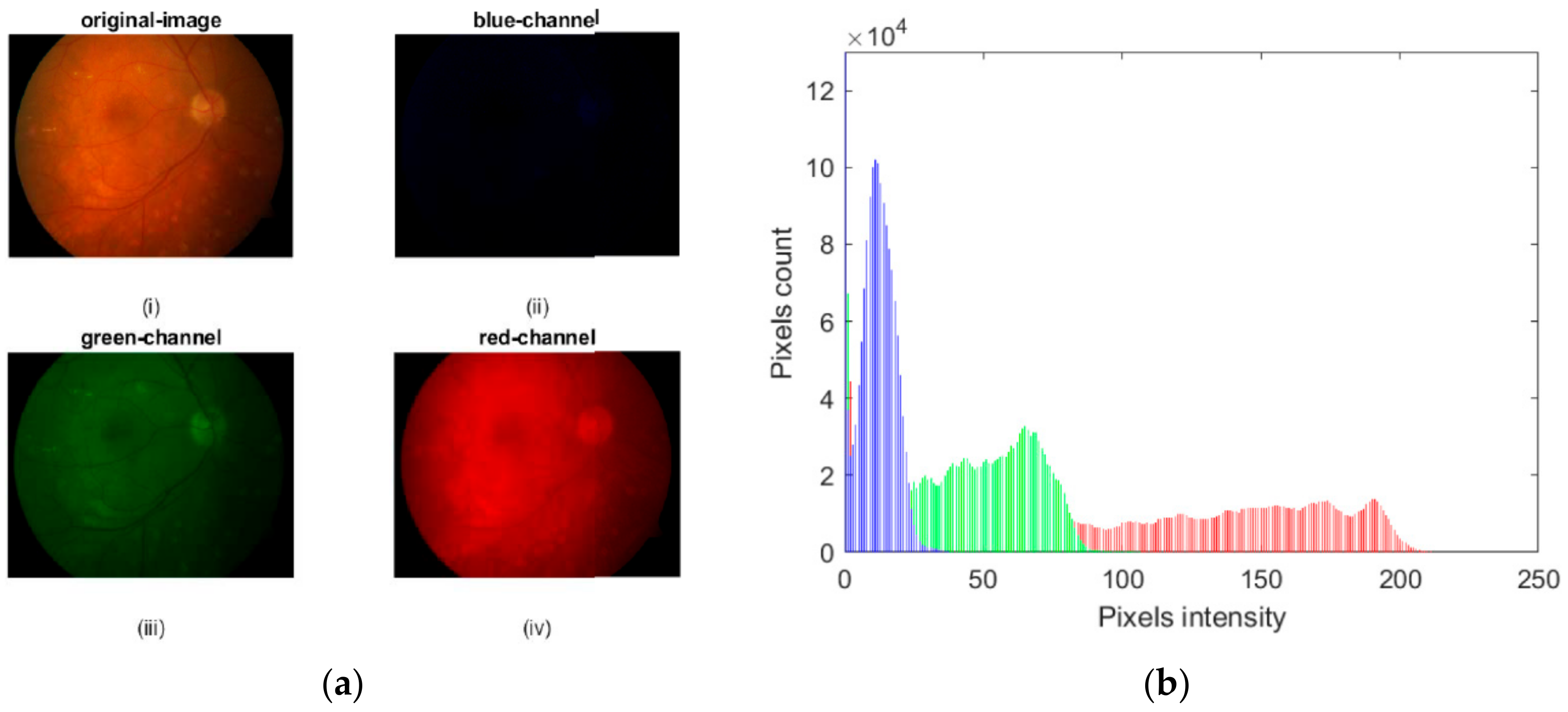
2.1. Preprocessing Based on Histogram
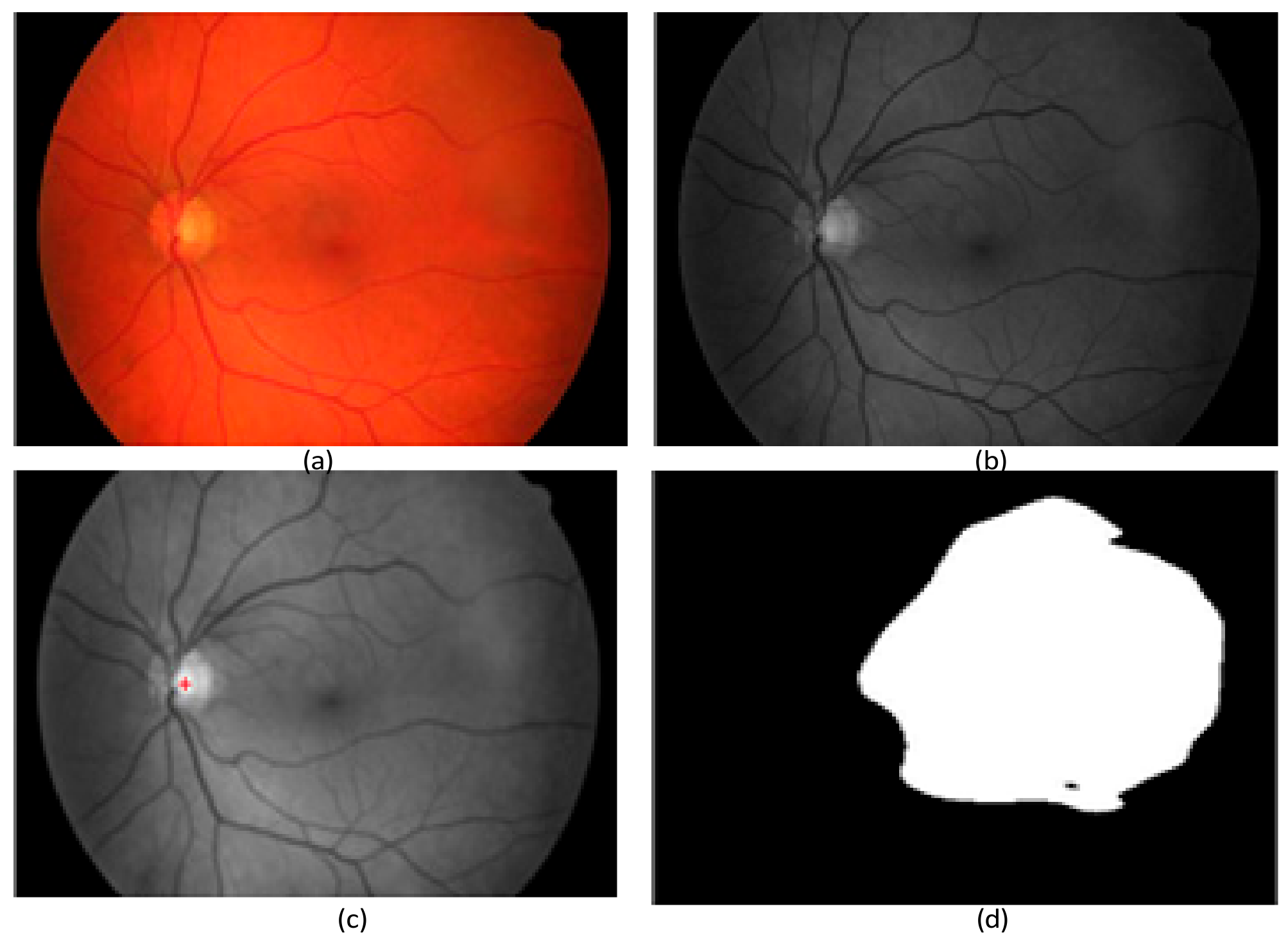
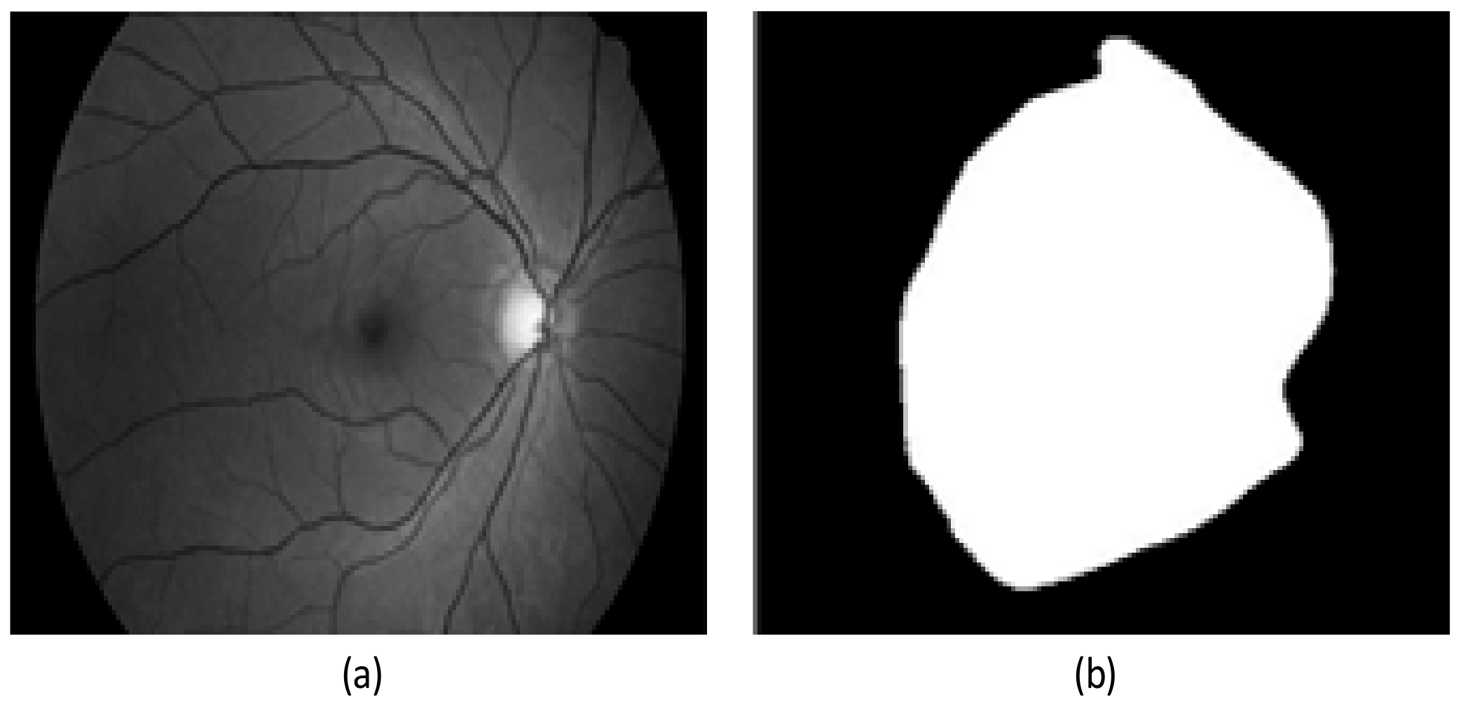
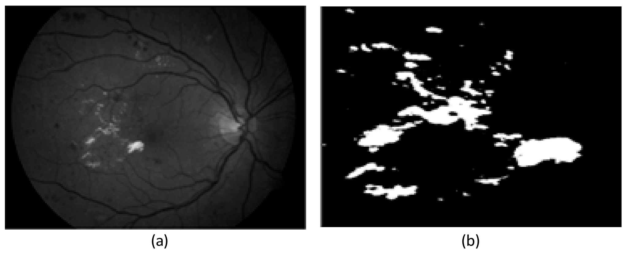
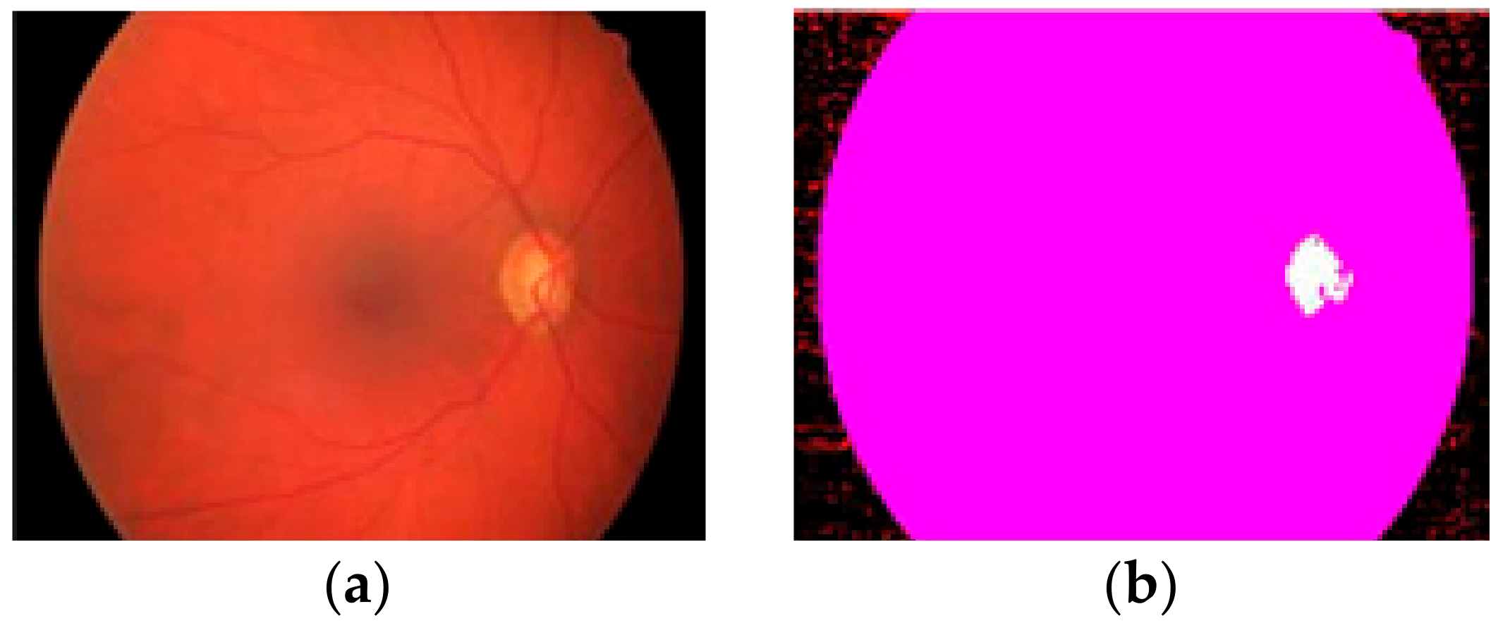
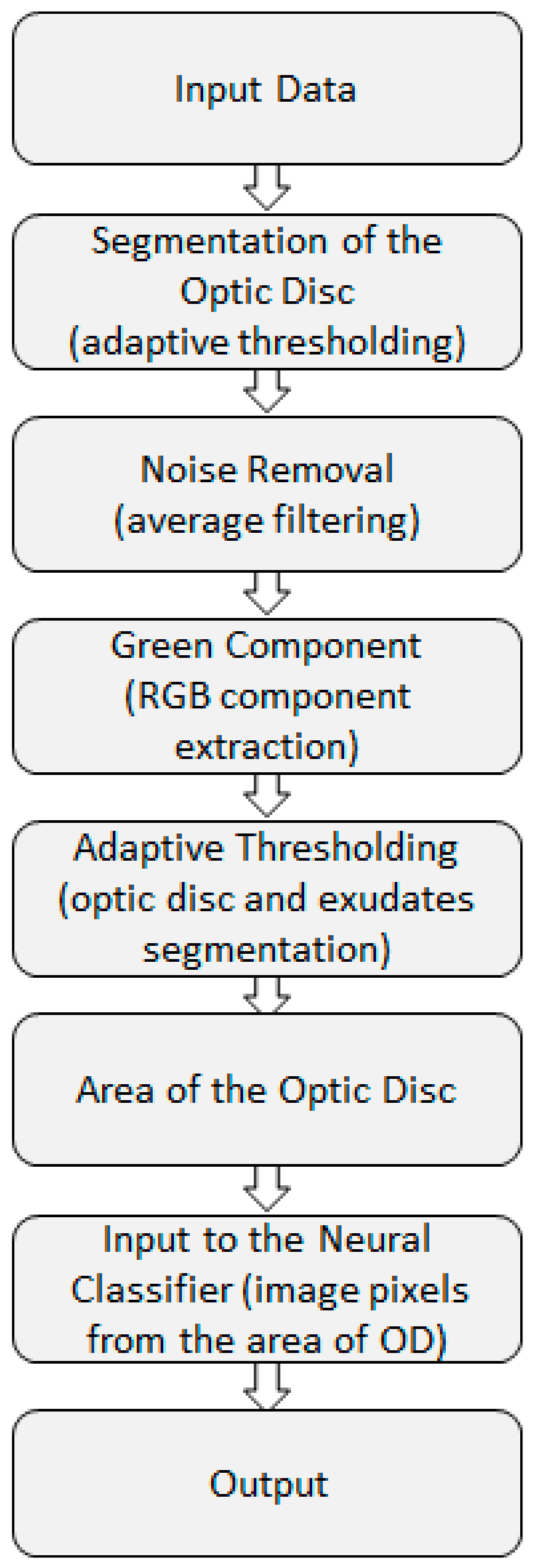
2.2. Preprocessing Based on Adaptive Thresholding
2.3. Preprocessing Based on Discrete Wavelet Transform (DWT)
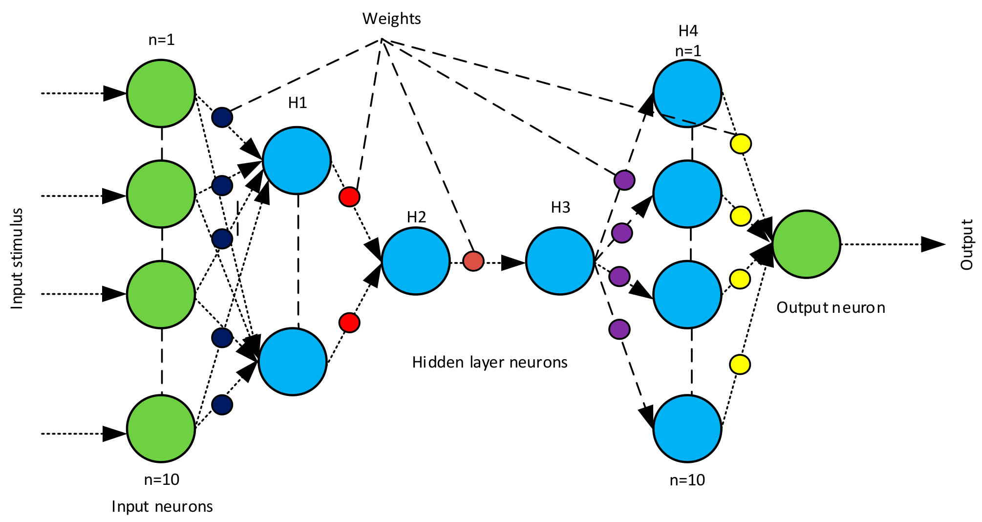
2.4. Backend Recognition Using a Neural Classifier
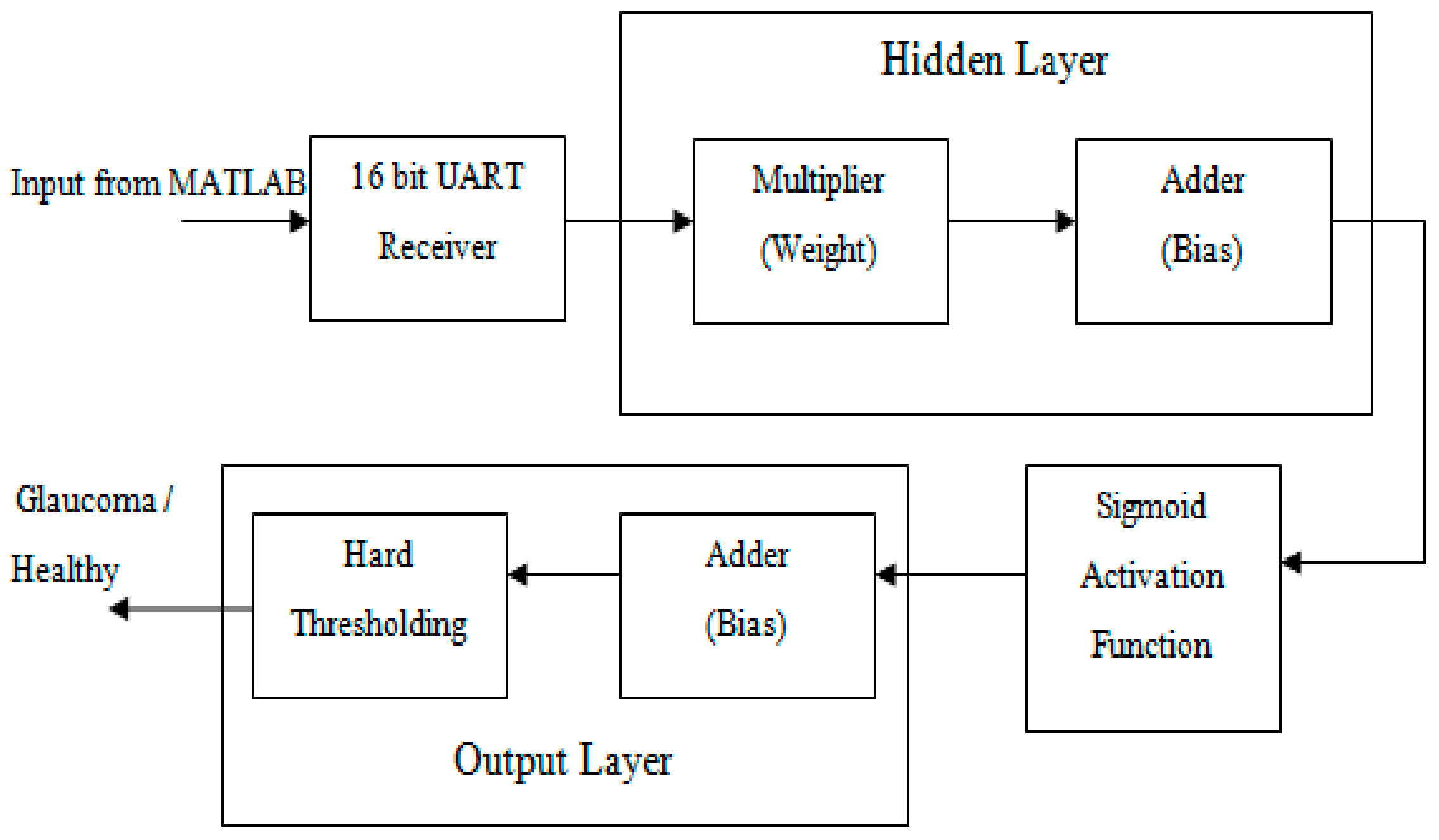
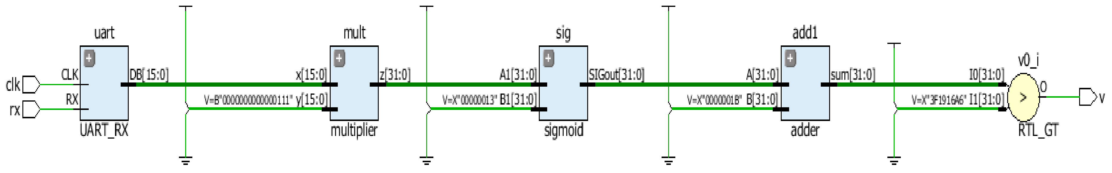
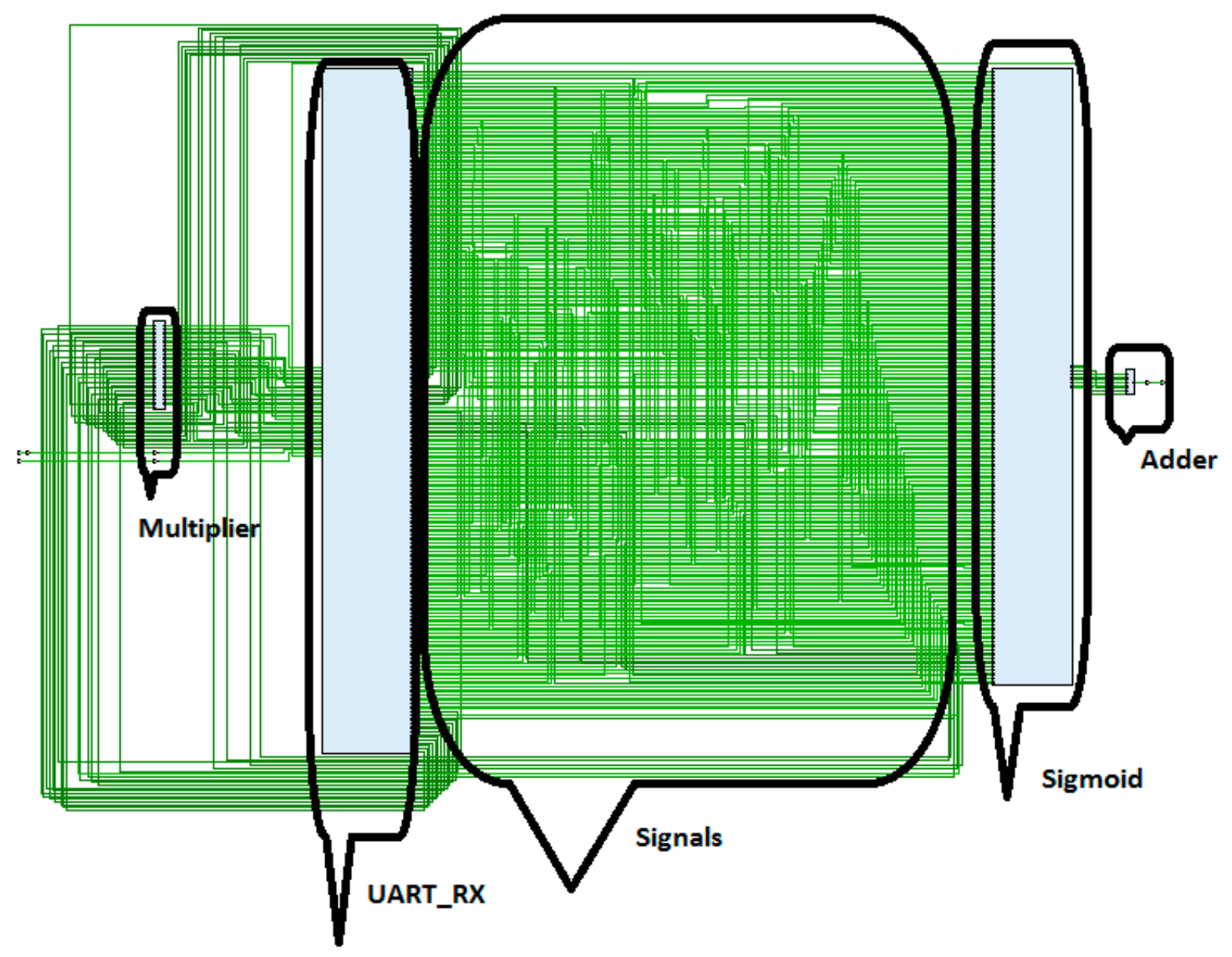
2.5. Hardware Implementation
3. Results and Discussion
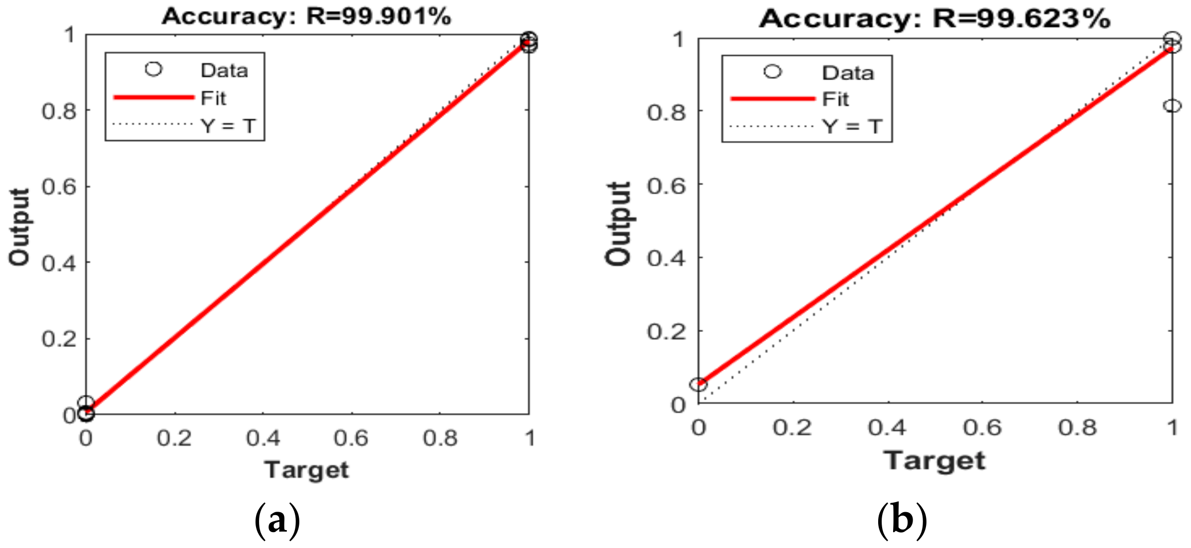
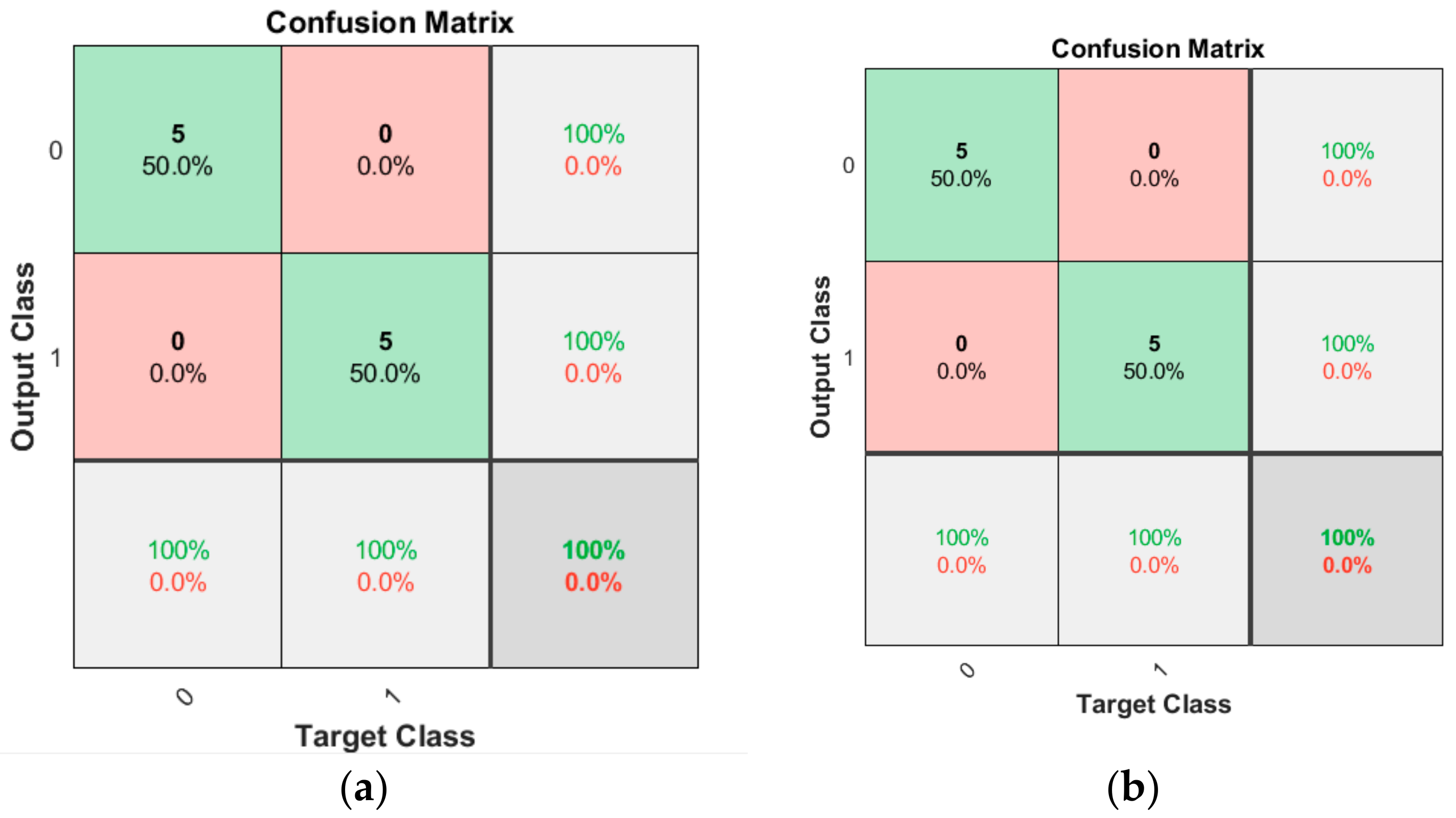
3.1. Software Implementation Results
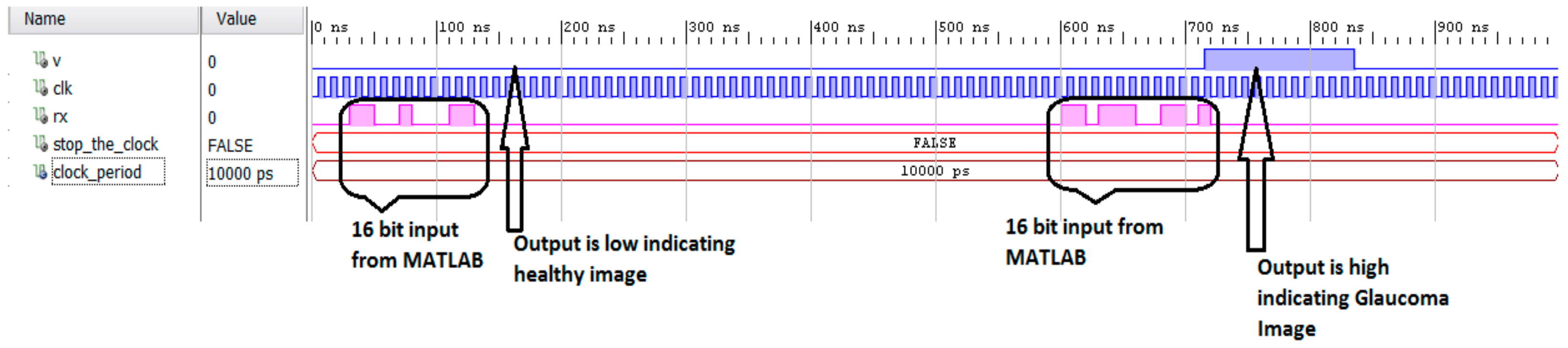
3.2. Hardware Implementation Results
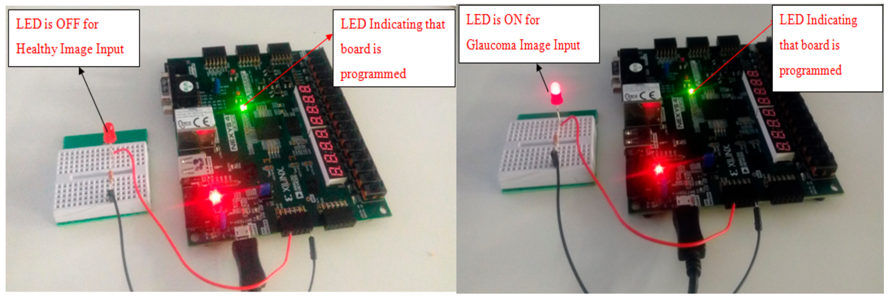
3.3. Experimental Setup
4. Conclusions
Author Contributions
Funding
Acknowledgments
Conflicts of Interest
References
- World Health Organization. Global Prevalence of Diabetes. Available online: https://www.who.int/diabetes/facts/en/diabcare0504.pdf (accessed on 20 October 2019).
- Khalid, S.; Akram, M.S.; Hassan, T.; Nasim, A.; Jameel, A. Fully Automated Robust System to Detect Retinal Edema, Central Serous Chorioretinopathy, and Age Related Macular Degeneration from Optical Coherence Tomography Images. BioMed Res. Int. 2017, 2017, 7148245. [Google Scholar] [CrossRef]
- Mary, M.C.V.S.; Rajsingh, E.B.; Naik, G.R. Retinal Fundus Image Analysis for Diagnosis of Glaucoma: A Comprehensive Survey. IEEE Access 2016, 4, 4327–4354. [Google Scholar] [CrossRef]
- Karami, N.; Rabbani, H. A dictionary learning based method for detection of diabetic retinopathy in color fundus images. In Proceedings of the 10th Iranian Conference on Machine Vision and Image Processing (MVIP), Isfahan, Iran, 22–23 November 2017; pp. 119–122. [Google Scholar]
- Zhou, L.; Zhao, Y.; Yang, J.; Yu, Q.; Xu, X. Deep multiple instance learning for automatic detection of diabetic retinopathy in retinal images. IET Image Process. 2018, 12, 563–571. [Google Scholar] [CrossRef]
- Chang, S.H.L.; Lee, Y.; Wu, S.; See, C.C.; Yang, M.; Lai, C.; Wu, W. Anterior Chamber Angle and Anterior Segment Structure of Eyes in Children with Early Stages of Retinopathy of Prematurity. Am. J. Ophthalmol. 2017, 179, 46–54. [Google Scholar] [CrossRef] [PubMed]
- National Eye Institute. Available online: https://nei.nih.gov/ (accessed on 20 October 2019).
- Kohler, T.; Budai, A.; Kraus, M.F.; Odstrcilik, J.; Michelson, G.; Hornegger, J. Automatic no-reference quality assessment for retinal fundus images using vessel segmentation. In Proceedings of the 26th IEEE International Symposium on Computer-Based Medical Systems, Porto, Portugal, 20–22 June 2013; Volume 1, pp. 95–100. [Google Scholar]
- Bharkad, S.D. Automatic Segmentation of Optic Disk in Retinal Images Using DWT. In Proceedings of the 2016 IEEE 6th International Conference on Advanced Computing (IACC), Bhimavaram, India, 27–28 February 2016; Volume 1, pp. 100–106. [Google Scholar] [CrossRef]
- Ravishankar, S.; Jain, A.; Mittal, A. Automated feature extraction for early detection of diabetic retinopathy in fundus images. In Proceedings of the IEEE Conference on Computer Vision and Pattern Recognition (CVPR), Miami, FL, USA, 20–25 June 2009; pp. 210–217. [Google Scholar]
- Sinthanayothin, C.; Boyce, J.F.; Williamson, T.H.; Cook, H.L.; Mensah, E.; Lal, S.; Usher, D. Automated detection of diabetic retinopathy on digital fundus images. Diabet. Med. 2002, 19, 105–112. [Google Scholar] [CrossRef]
- Faust, O.; Acharya, R.U.; Ng, E.Y.K.; Ng, K.; Suri, J.S. Algorithms for the automated detection of diabetic retinopathy using digital fundus images: A review. J. Med. Syst. 2012, 36, 145–157. [Google Scholar] [CrossRef]
- Nayak, J.; Bhat, P.S.; Acharya, R.; Lim, C.M.; Kagathi, M. Automated identification of diabetic retinopathy stages using digital fundus image. J. Med. Syst. 2008, 32, 107–115. [Google Scholar] [CrossRef]
- Ramaswamy, M.; Anitha, D.; Kuppamal, S.P.; Sudha, R.; Mon, S.F.A. A study and comparison of automated techniques for exudate detection using digital fundus images of human eye: A review for early identification of diabetic retinopathy. Int. J. Comput. Technol. Appl. 2011, 2, 1503–1516. [Google Scholar]
- Acharya, U.R.; Lim, C.M.; Ng, E.Y.K.; Chee, C.; Tamura, T. Computer-based detection of diabetes retinopathy stages using digital fundus images. Proc. Inst. Mech. Eng. 2009, 223, 545–553. [Google Scholar] [CrossRef]
- Hansen, A.B.; Hartvig, N.V.; Jensen, M.S.J.; Borch-Johnsen, K.; Lund-Andersen, H.; Larsen, M. Diabetic retinopathy screening using digital non-mydriatic fundus photography and automated image analysis. Acta Ophthalmol. Scand. 2004, 82, 666–672. [Google Scholar] [CrossRef]
- Zhang, X.; Chutape, O. A SVM approach for detection of hemorrhages in background diabetic retinopathy. In Proceedings of the International Joint Conference on Neural Networks, Montreal, QC, Canada, 31 July–4 August 2005; pp. 2435–2440. [Google Scholar]
- Kahaki, S.M.; Nordin, M.J.; Ahmad, N.S.; Arzoky, M.; Ismail, W. Deep convolutional neural network designed for age assessment based on orthopantomography data. Neural Comput. Appl. 2019. [Google Scholar] [CrossRef]
- Odstrcilik, J.; Kolar, R.; Budai, A.; Hornegger, J.; Jan, J.; Gazarek, J.; Kubena, T.; Cernosek, P.; Svoboda, O.; Angelopoulou, E. Retinal vessel segmentation by improved matched filtering: Evaluation on a new high-resolution fundus image database. IET Image Process. 2013, 7, 373–378. [Google Scholar] [CrossRef]
- Mudassar, A.A.; Butt, S. Extraction of Blood Vessels in Retinal Images Using Four Different Techniques. J. Med. Eng. 2013, 2013, 408120. [Google Scholar] [CrossRef] [PubMed]
- Bradley, D.; Roth, G. Adaptive Thresholding Using the Integral Image. 2005. Available online: http://www.scs.carleton.ca/~roth/iit-publications-iti/docs/gerh-50002.pdf (accessed on 25 October 2019).
- Agarwal, A.; Gulia, S.; Chaudhary, S.; Dutta, M.K.; Burget, R.; Riha, K. Automatic glaucoma detection using adaptive threshold based technique in fundus image. In Proceedings of the 2015 38th International Conference on Telecommunications and Signal Processing (TSP), Prague, Czech Republic, 9–11 July 2015; pp. 416–420. [Google Scholar]
- Yun, W.L.; Acharya, U.R.; Venkatesh, Y.; Chee, C.; Min, L.C.; Ng, E. Identification of different stages of diabetic retinopathy using retinal optical images. Inf. Sci. 2008, 178, 106–121. [Google Scholar] [CrossRef]
- Magoulas, G.D.; Prentza, A. Machine Learning and Its Applications Lecture Notes in Computer Science; Springer: Berlin/Heidelberg, Germany, 2011; pp. 300–307. [Google Scholar]
- El-Sappagh, S.; Elmogy, M.; Ali, F.; Abuhmed, T.; Islam, S.M.; Kwak, K.S. A Comprehensive Medical Decision–Support Framework Based on a Heterogeneous Ensemble Classifier for Diabetes Prediction. Electronics 2019, 8, 635. [Google Scholar] [CrossRef]
- Ashfaq, M.; Minallah, N.; Ullah, Z.; Ahmad, A.M.; Saeed, A.; Hafeez, A. Performance Analysis of Low-Level and High-Level Intuitive Features for Melanoma Detection. Electronics 2019, 8, 672. [Google Scholar] [CrossRef]
- Vununu, C.; Lee, S.H.; Kwon, K.R. A Deep Feature Extraction Method for HEp-2 Cell Image Classification. Electronics 2019, 8, 20. [Google Scholar] [CrossRef]
- Niemeijer, M.; van Ginneken, B.; Staal, J.; Suttorp-Schulten, M.S.A.; Abramoff, N.D. Automatic detection of red lesion in digital color fundus photographs. IEEE Trans. Med. Imaging 2005, 24, 584–592. [Google Scholar] [CrossRef]
- Xilinx. Available online: https://www.xilinx.com/products/silicon-devices/fpga/artix-7.html (accessed on 23 October 2019).
- Ide, A.N.; Saito, J.H. FPGA Implimentations of Neocognitrons; Springer: Berlin/Heidelberg, Germany, 2006; pp. 197–224. [Google Scholar]
- Aquino, A.; Gegúndez-Arias, M.E.; Marín, D. Detecting the optic disc boundary in digital fundus images using morphological, edge, detection, and feature extraction techniques. IEEE Trans. Med. Imaging 2010, 29, 1860–1869. [Google Scholar] [CrossRef]
- Kahaki, S.M.M.; Nordin, M.J.; Ismail, W.; Zahra, S.J.; Hassan, R. Blood cancer cell classification based on geometric mean transform and dissimilarity metrics. Pertanika J. Sci. Technol. 2017, 25, 223–234. [Google Scholar]
- Hoover, A.; Goldbaum, M. Locating the optic nerve in a retinal image using the fuzzy convergence of the blood vessels. IEEE Trans. Med. Imaging 2003, 22, 951–958. [Google Scholar] [CrossRef] [PubMed]
- Xilinx. Available online: https://www.xilinx.com/products/design-tools/vivado.html (accessed on 20 October 2019).
- Nieto, A.; Brea, V.M.; Vilariño, D.L. FPGA-accelerated retinal vessel-tree extraction. In Proceedings of the 2009 IEEE International Conference on Field Programmable Logic and Applications, Prague, Czech Republic, 31 August–2 September 2009; pp. 485–488. [Google Scholar]
- Koukounis, D.; Tttofis, C.; Theocharides, T. Hardware acceleration of retinal blood vasculature segmentation. In Proceedings of the 23rd ACM International Conference on Great Lakes Symposium on VLSI, Paris, France, 2–4 May 2013; pp. 113–118. [Google Scholar]
- Cavinato, L.; Fidone, I.; Bacis, M.; Del Sozzo, E.; Durelli, G.C.; Santambrogio, M.D. Software implementation and hardware acceleration of retinal vessel segmentation for diabetic retinopathy screening tests. In Proceedings of the 2017 39th Annual International Conference of the IEEE Engineering in Medicine and Biology Society (EMBC), Jeju Island, Korea, 11–15 July 2017; pp. 1–4. [Google Scholar]


| Reference | Methodology | Features Used | Test Cases Analysed | Accuracy |
|---|---|---|---|---|
| [31] | Edge detection | Circular Hough transform | Not reported (segmentation algorithm applied on all images) | 86% accuracy |
| [33] | Fuzzy convergence of blood vessels | Blood Vessel convergence illumination equalisation | 81 samples for both healthy and diseased retina | 89% accuracy |
| [22] | Histogram analysis, adaptive thresholding | Mean, standard deviation and cup-disk ratio | 20 samples in total for glaucoma and healthy images | 90% accuracy |
| Proposed Method | Adaptive Thresholding | Area of the segmented OD | 15 samples for glaucoma, healthy and DR | 100% accuracy |
| Logic Operator | Slice (LUT) 63400 |
|---|---|
| Total utilisation | 2048 (3.23%) |
| Adder | 10 (0.02%) |
| Embedded Multiplier | 0 |
| Sigmoid | 1797 (2.835) |
| UART | 243 (0.38%) |
| Total On-Chip Power | 13.776 W |
|---|---|
| Static Power Consumption | 0.293 W (2% of total) |
| Dynamic Power Consumption | 13.484 W (98% of total) |
| Platform | PC/Device | Execution Time | Power Consumption |
|---|---|---|---|
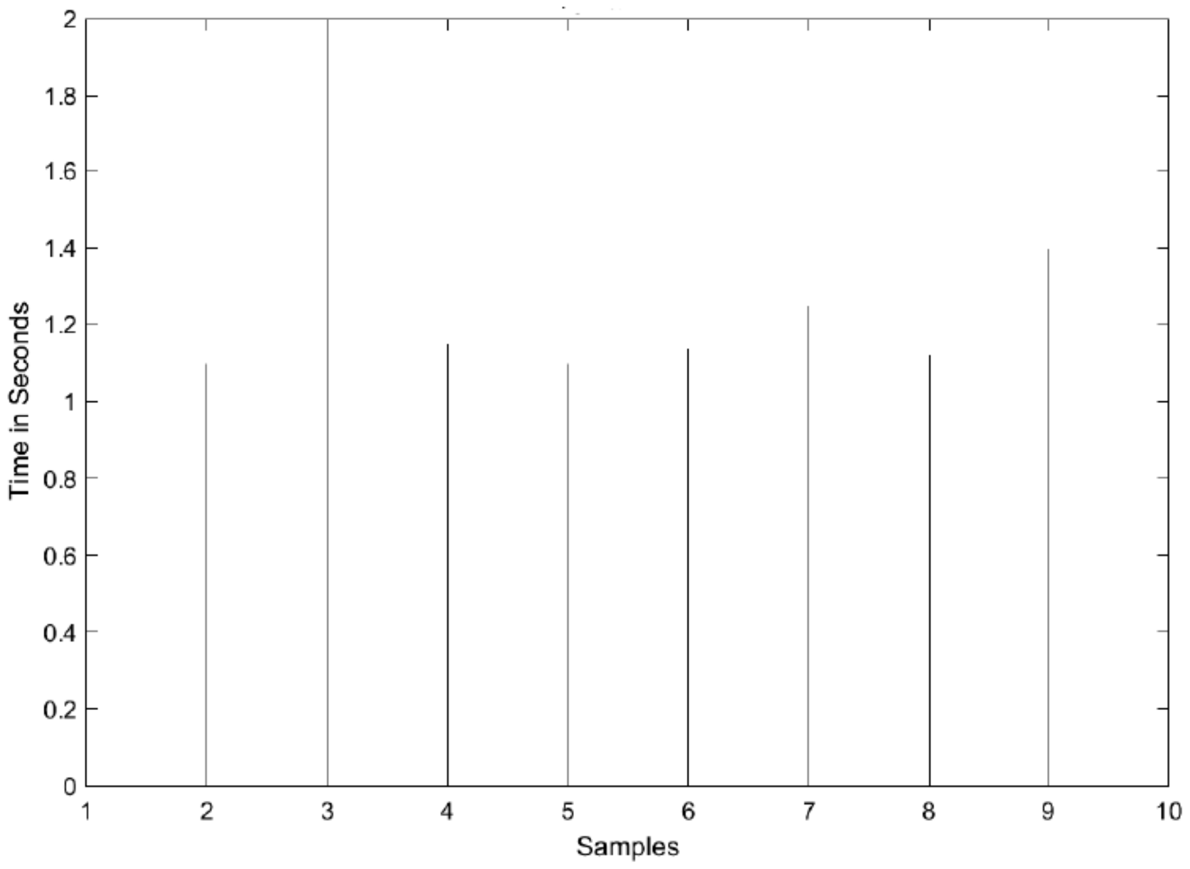
| Software | Intel i5-6200 | 1.2 s/sample | 25.656 W |
| Hardware | Nexys4 DDR | 400 ns/sample | 11.776 W |
© 2019 by the authors. Licensee MDPI, Basel, Switzerland. This article is an open access article distributed under the terms and conditions of the Creative Commons Attribution (CC BY) license (http://creativecommons.org/licenses/by/4.0/).
Share and Cite
Ghani, A.; See, C.H.; Sudhakaran, V.; Ahmad, J.; Abd-Alhameed, R. Accelerating Retinal Fundus Image Classification Using Artificial Neural Networks (ANNs) and Reconfigurable Hardware (FPGA). Electronics 2019, 8, 1522. https://doi.org/10.3390/electronics8121522
Ghani A, See CH, Sudhakaran V, Ahmad J, Abd-Alhameed R. Accelerating Retinal Fundus Image Classification Using Artificial Neural Networks (ANNs) and Reconfigurable Hardware (FPGA). Electronics. 2019; 8(12):1522. https://doi.org/10.3390/electronics8121522
Chicago/Turabian StyleGhani, Arfan, Chan H. See, Vaisakh Sudhakaran, Jahanzeb Ahmad, and Raed Abd-Alhameed. 2019. "Accelerating Retinal Fundus Image Classification Using Artificial Neural Networks (ANNs) and Reconfigurable Hardware (FPGA)" Electronics 8, no. 12: 1522. https://doi.org/10.3390/electronics8121522
APA StyleGhani, A., See, C. H., Sudhakaran, V., Ahmad, J., & Abd-Alhameed, R. (2019). Accelerating Retinal Fundus Image Classification Using Artificial Neural Networks (ANNs) and Reconfigurable Hardware (FPGA). Electronics, 8(12), 1522. https://doi.org/10.3390/electronics8121522