Role of the Product λ^′(0)ρ^′(1) in Determining LDPC Code Performance

Abstract

The objective of this work is to analyze the importance of the product ${\lambda }^{\prime }(0){\rho }^{\prime }(1)$ in determining low density parity check (LDPC) code performance, as far as its influence on the weight distribution function and on the decoding thresholds. This analysis is based on the 2006 paper by Di et al., as far as the weight distribution function is concerned, and on the 2018 paper by Vatta et al., regarding the LDPC decoding thresholds. In particular, the first paper Di et al. analyzed the relation between the above mentioned product and the minimum weight of an ensemble of random LDPC codewords, whereas in the second some analytical upper bounds to the LDPC decoding thresholds were determined. In the present work, besides analyzing the performance of an ensemble of LDPC codes through the outcomes of Di et al.’s 2006 paper, we give the relation between one of the upper bounds found in Vatta et al.’s 2018 paper and the above mentioned product ${\lambda }^{\prime }(0){\rho }^{\prime }(1)$, thus showing its role in also determining an upper bound to LDPC decoding thresholds.

1. Introduction

Low Density Parity Check (LDPC) codes, belonging to the class of block channel codes, were introduced for the first time in the 1960s in Robert Gallager’s doctoral thesis [1]. Now they are counted among the most promising and cutting-edge coding techniques in contemporary channel coding. Due to the technological impediments of the time in which they were introduced and of the decoder complexity, these codes were hardly contemplated for about 30 years, with the exception of Tanner’s graphical description, introduced in [2], and successively designated as the Tanner graph. Appearing independently of Gallager’s work, the authors of [3,4] were the re-inventors of LDPC codes in the mid 1990s. Afterwards, because of their astonishing performance approaching the Shannon limit along with Turbo codes [5], they were rapidly comprehended in current communication standards [6,7,8].

The asymptotic performance of a block channel code, such as an LDPC code, is determined by its minimum distance, i.e., by its minimum weight codewords and by their multiplicities. These determine its correction capability and its asymptotic performance expressed in terms of bit error rate (BER) and frame error rate (FER) vs. the signal-to-noise ratio (SNR) $E_b/N_0$ from moderate to high SNRs, i.e., away from capacity. Moreover, as far as LDPC codes are concerned, as first observed in [1], it presents the well-known “threshold phenomenon”. In other words, the noise threshold defines a channel noise upper bound under which the lost information probability can be maintained as low as needed.

Since it is extremely difficult to study the performance of a LDPC codes ensemble analytically as the determination of its weight enumerating function is a complicated task, in this work we try to give an insight into this problem analyzing the importance of the product ${\lambda }^{\prime }(0){\rho }^{\prime }(1)$ in influencing not only this function, that, as said above, determines the asymptotic BER and FER performance, away from capacity, but also the decoding thresholds, i.e., the performance next to the Shannon limit. Namely, on the basis of the results of [9,10], respectively, we are interested in determining, on one side, the relationship between the above mentioned product and the minimum distance of a LDPC codes ensemble, and, on the other side, the relationship between this product and the noise threshold of a LDPC codes ensemble. The first, namely the minimum distance, is related to LDPC’s codewords weight distribution, i.e., to their distance spectrum. The second, namely the noise threshold, is related to the convergence behavior of their iterative decoding algorithm, which is particularly important because LDPC codes, as well as turbo-like codes, are “capacity-achieving” codes.

As far as the first of the above cited papers, namely [9], is concerned, its main result asserts that the minimum distance growth rate of irregular LDPC codes ensembles is only determined by the value of the product ${\lambda }^{\prime }(0){\rho }^{\prime }(1)$, a number that is related to the degree distribution polynomial couple $\lambda (x)$ and $\rho (x)$. In particular, if ${\lambda }^{\prime }(0){\rho }^{\prime }(1)>1$, the minimum distance growth with the block length being sublinear, if not, the minimum distance growth with the block length is linear.

As far as the second of the above cited papers, namely Vatta et al.’s 2018 paper [10], is concerned, in this work we derived three computationally light upper bounds to LDPC belief-propagation decoding thresholds, usually determined “exactly” through density evolution, assuming, as in [11], the validity of the Gaussian Approximation (GA) (the employment of which is very convenient when an effective and computationally light method is required. See [10,12,13,14,15]), and by using the derivation of [16] (the clarifying vision and interpretation of [11] allows to determine the threshold as the ultimate value guaranteeing the convergence of the recurrent sequence, therein defined, but the authors of [11] did not provide any mathematical method to calculate it. Thus, in [16] we presented a mathematical method, based on the quadratic degeneracy theory, allowing the evaluation of noise thresholds by means of converting a convergence problem into a mathematical analysis problem. Using the algorithm shown in [16], a computationally light approximation of LDPC belief-propagation decoding thresholds, usually determined “exactly” through density evolution, can be obtained, assuming, as in [11], the validity of the GA) to determine the asymptotic analytical performance of $\Delta (s,t)$ defined, e.g., in [6].

In Section 2 we recall LDPC codes graphical representation and, in Section 3, the Gaussian Approximation approach. In Section 4 we review the mathematical method deduced in [16] to explain how the upper bounds of [10] were obtained. Furthermore, to analyze the relationship between the product ${\lambda }^{\prime }(0){\rho }^{\prime }(1)$ and the minimum distance of a LDPC codes ensemble, in Section 6 the results of [9] are recalled, and, to analyze the relationship between this product and the noise threshold of a LDPC codes ensemble, in Section 7 we present a Lemma specifying the relationship between the third noise threshold upper bound found in [10] and the product ${\lambda }^{\prime }(0){\rho }^{\prime }(1)$. In Section 8, the numeric results of these two analyses are reported. These results are discussed in Section 9 which also will report some simulation results to support the discussion. Finally, Section 10 summarizes the conclusions.

2. Graphical Representation of LDPC Codes

LDPC codes can be represented in a graphical way through a commonly named bipartite graph, commonly known as the Tanner graph [2]. As the trellis diagram gives an efficient graphical representation of a convolutional code behavior, so does the Tanner graph in providing an efficient graphical representation of how a LDPC encoder and decoder work.

The nodes in a Tanner graph are classified in variable nodes and check nodes. In the drawing of the Tanner graph, the following rule must be respected: An edge connects a variable node i to a check node j when the corresponding element $h_{ij}$ in the parity-check matrix H is a 1. From this it may be deduced that there is a check node for each of the $m=n-k$ check equations, and that there is a variable node for each of the n code bits $c_i$.

As far as irregular LDPC codes are concerned [4], the parameters $d_l$ and $d_r$ specify the maximum degrees of the nodes distributions in their Tanner graphs, defined, e.g., in [17]. In particular, the polynomial $\lambda (x)$ ($\rho (x)$) defines the variable (check) nodes edge-perspective degree distribution:

$$\lambda (x)=\sum _{i=2}^{d_l}{\lambda }_i{x}^{i-1}$$

(1)

$$\rho (x)=\sum _{j=2}^{d_r}{\rho }_j{x}^{j-1}$$

(2)

A LDPC code rate can be expressed as [18]:

$$r(\lambda ,\rho )=1-\frac{{\int }_0^1\rho (x)\mathrm{d}x}{{\int }_0^1\lambda (x)\mathrm{d}x}=1-\frac{{\sum }_{j=2}^{d_r}{\rho }_j/j}{{\sum }_{j=2}^{d_l}{\lambda }_j/j}$$

(3)

The edge-perspective degree distributions $\lambda (x)$ and $\rho (x)$ are related to the node perspective degree distributions $L(x)$ and $R(x)$ as follows [9]:

$$L(x)=\sum _{i=2}^{d_l}{L}_i{x}^i$$

(4)

$$R(x)=\sum _{j=2}^{d_r}{R}_j{x}^j$$

(5)

being,

$$L_j=\frac{{\lambda }_j}{j{\int }_0^1\lambda (x)}=\frac{{\lambda }_j/j}{{\sum }_{i=2}^{d_l}{\lambda }_i/i}$$

(6)

$$R_j=\frac{{\rho }_j}{j{\int }_0^1\rho (x)}=\frac{{\rho }_j/j}{{\sum }_{i=2}^{d_r}{\rho }_i/i}.$$

(7)

3. Gaussian Approximation

Following the assumptions made in [11], the distributions of the messages involved in the LDPC iterative decoding process under appropriate hypotheses may be approximated as Gaussians. Since it may be observed that to totally specify a Gaussian only its mean and variance are needed, and during the iterative decoding process it is necessary to specify only the means and variances of a generic check node output message, u, and of a generic variable node output message, v. Furthermore, since in [11], assuming the validity of the symmetry condition, the variance ${\sigma }^2$ was shown to be connected to the mean m by the relation ${\sigma }^2=2m$, the means only can be kept in the computation process. The means of u and v have been denoted by $m_u^{(l)}$ and $m_v^{(l)}$ at the l-th iteration, respectively. Furthermore, the log-likelihood ratio (LLR) message $u_0$ from the channel can be taken as Gaussian with a mean of $m_{u_0}=2/{\sigma }_n^2$ and a variance of $4/{\sigma }_n^2$, being ${\sigma }_n^2=N_0/2$ the variance of the channel noise.

The mean of the output of a degree-i variable node at the $l^{th}$ iteration is:

$$m_{v,i}^{(l)}=m_{u_0}+(i-1)m_u^{(l-1)}$$

(8)

where $m_{u_0}$ is the mean of $u_0$ and $m_u^{(l-1)}$ is the mean of u at the $(l-1)$-th iteration.

Defining $\varphi (x)$ as in Definition 1 in [11], the update rule for an irregular code becomes:

$$m_{u,j}^{(l)}={\varphi }^{-1}\left(1-{\left[1-\sum _{i=2}^{d_l}{\lambda }_i\varphi (m_{v,i}^{(l)})\right]}^{j-1}\right).$$

(9)

The output of a variable node is specified by its mean $m_u^{(l)}$, that can be calculated as the linear combination of the means $m_{u,j}^{(l)}$:

$$m_u^{(l)}=\sum _{j=2}^{d_r}{\rho }_j{\varphi }^{-1}\left(1-{\left[1-\sum _{i=2}^{d_l}{\lambda }_i\varphi \left(m_{u_0}+(i-1)m_u^{(l-1)}\right)\right]}^{j-1}\right).$$

(10)

Defining $s=m_{u_0}$ and $t_l=m_u^{(l)}$, Equation (10) may be rewritten as:

$$t_l=f(s,t_{l-1})$$

(11)

where the function $f(s,t)$ is expressed as:

$$f_j(s,t):={\varphi }^{-1}\left(1-{\left[1-\sum _{i=2}^{d_l}{\lambda }_i\varphi (s+(i-1)t)\right]}^{j-1}\right)$$

(12)

$$f(s,t):=\sum _{j=2}^{d_r}{\rho }_j{f}_j(s,t).$$

(13)

4. Mathematical Method of [16]

As noted in [16], the problem of the determination of the convergence of Equation (10) may be solved by converting it to a problem of quadratic degeneracy, the solution of which can be given in charge to a commercial software. If the second partial derivative of $f(s,t)$ with respect to t, $f_{tt}(s,t)$, is $\ne 0$, the problem of the determination of the convergence of Equation (10) becomes the search for the solution of the following system:

$$\left\{\begin{array}{c}f(s,t)=t\hfill \\ f_t(s,t)=1\hfill \end{array}\right.$$

(14)

where $f_t(s,t)$ is the first partial derivative of $f(s,t)$ with respect to t. Its solution is the value $s^{*}=m_{u_0}^{*}$, which is the minimum $s=m_{u_0}$ guaranteeing the convergence of Equation (10).

Defining, as in [6],

$$\Delta (s,t):=f(s,t)-t$$

(15)

and

$${\Delta }_t(s,t)=f_t(s,t)-1$$

(16)

Equation (14) is given by:

$$\left\{\begin{array}{c}\Delta (s,t)=0\hfill \\ {\Delta }_t(s,t)=0\hfill \end{array}\right.$$

(17)

Its solution $(s^{*},t^{*})$ gives an estimate of the belief-propagation decoding threshold ${\sigma }^{*}:=\sqrt{\frac{2}{s^{*}}}$ that may be determined exactly using density evolution. To solve Equation (17), an invertible approximation of the function $\varphi (x)$ is needed (see, e.g., [11,19,20]).

5. Upper Bounds on LDPC Codes Decoding Thresholds

The upper bounds on thresholds have been determined in [10] from the asymptotic performance of Equation (17). The first bound, called $s_{\mathrm{bound}}^{*}$ in [10], was obtained determining an approximation of the function $\varphi (x)$ valid for when $x\ge 10$. To obtain the second upper bound, called $s_{\mathrm{approx}}^{*}$ in [10], we have used the approximation Equation (16) of [10] (that was implicitly used in [11]). Finally, involving the Jensen’s inequality to manipulate the second upper bound, the third bound, called $s_{\mathrm{Jensen}}^{*}$ in [10], was determined.

5.1. Upper Bound on LDPC Codes Decoding Thresholds Holding for $i_1\ge 2$

As far as the above mentioned first upper bound on LDPC codes thresholds (called $s_{\mathrm{bound}}^{*}$ in [10]) is concerned, in [20] the following lemma was proved.

Lemma: Given $\lambda (x)$ of minimum degree $i_1\ge 2$, and defining $z(s,t)$ as $z(s,t):=\frac{s+(i_1-1)t}{2}$ and $A_j$ as $A_j:=\frac{1}{{(j-1)}^2{\lambda }_{i_1}^2}$, being $\mathrm{W}(·)$ the Lambert-W function, the following asymptotic approximation holds:

$$f(s,t)=2\sum _{j=2}^{d_r}{\rho }_j\mathrm{W}(A_{j}z(s,t){\mathrm{e}}^{z(s,t)})+O(t^{-1}).$$

(18)

Recalling that $\frac{\mathrm{d}\mathrm{W}(x)}{\mathrm{d}x}=\frac{1}{x+{\mathrm{e}}^{\mathrm{W}(x)}}$:

$$f_t(s,t)=2\sum _{j=2}^{d_r}{\rho }_j\frac{z_t(s,t){\mathrm{e}}^{z(s,t)}(1+z(s,t))}{z(s,t){\mathrm{e}}^{z(s,t)}+{\mathrm{e}}^{\mathrm{W}(A_{j}z(s,t){\mathrm{e}}^{z(s,t)})-\log A_j}}.$$

(19)

Applying Equation (14) to Equations (18) and (19) we get:

$$\left\{\begin{array}{c}2{\sum }_{j=2}^{d_r}{\rho }_j\mathrm{W}(A_{j}z(s,t){\mathrm{e}}^{z(s,t)})=t\hfill \\ 2{\sum }_{j=2}^{d_r}{\rho }_j\frac{z_t(s,t){\mathrm{e}}^{z(s,t)}(1+z(s,t))}{z(s,t){\mathrm{e}}^{z(s,t)}+{\mathrm{e}}^{\mathrm{W}(A_{j}z(s,t){\mathrm{e}}^{z(s,t)})-\log A_j}}=1\hfill \end{array}\right..$$

(20)

and Equation (17) can be rewritten as:

$$\left\{\begin{array}{c}2{\sum }_{j=2}^{d_r}{\rho }_j\mathrm{W}(A_{j}z(s,t){\mathrm{e}}^{z(s,t)})-t=0\hfill \\ 2{\sum }_{j=2}^{d_r}{\rho }_j\frac{z_t(s,t){\mathrm{e}}^{z(s,t)}(1+z(s,t))}{z(s,t){\mathrm{e}}^{z(s,t)}+{\mathrm{e}}^{\mathrm{W}(A_{j}z(s,t){\mathrm{e}}^{z(s,t)})-\log A_j}}-1=0\hfill \end{array}\right..$$

(21)

Its solution ($s_{\mathrm{bound}}^{*}$, $t_{\mathrm{bound}}^{*}$) determines the bound ${\sigma }_{\mathrm{bound}}^{*}=\sqrt{\frac{2}{s_{\mathrm{bound}}^{*}}}$, which is valid $\forall i_1$, unlike the other two ($s_{\mathrm{approx}}^{*}$ and $s_{\mathrm{Jensen}}^{*}$) reported in [10], which hold both for $i_1=2$ only.

5.2. Further Upper Bounds on LDPC Codes Decoding Thresholds Holding for $i_1=2$

With $a_j:=\log A_j=-2\log ((j-1){\lambda }_{i_1})$, Equation (18) can be rewritten as:

$$f(s,t)=2\sum _{j=2}^{d_r}{\rho }_j\mathrm{W}\left(z(s,t){\mathrm{e}}^{z(s,t)+a_j}\right)+O(t^{-1}).$$

(22)

Assuming that the following simplified approximation holds:

$$\mathrm{W}\left(z(s,t){\mathrm{e}}^{z(s,t)+a_j}\right)\simeq \mathrm{W}\left((z(s,t)+a_j){\mathrm{e}}^{z(s,t)+a_j}\right),$$

(23)

calling $x:=z_s(t)+a_j$, and being $W(x{\mathrm{e}}^x)\equiv x$ for $x>0$, we find a much simpler asymptotic expression for $f(s,t)$ (simpler than the one of Equation (18)):

$$f(s,t)\simeq 2\sum _{j=2}^{d_r}{\rho }_j\mathrm{W}\left((z(s,t)+a_j)e^{z(s,t)+a_j}\right)=2\sum _{j=2}^{d_r}{\rho }_j(z(s,t)+a_j)=\sum _{j=2}^{d_r}{\rho }_j(s+(i_1-1)t-4\log ((j-1){\lambda }_{i_1})).$$

(24)

Thus, the asymptotic performance of $f(s,t)$ is given by:

$$f(s,t)=s+(i_1-1)t-4\log {\lambda }_{i_1}-4\sum _{j=2}^{d_r}{\rho }_j\log (j-1)+O(t^{-1}).$$

(25)

This is the same asymptotic expression obtained, following a different derivation, in [11], where the approximation in Equation (23) was implicitly used in the proof of Lemma 3.

Thus, ignoring the $O(t^{-1})$, for large t Equation (17) can be rewritten as:

$$\left\{\begin{array}{c}s+(i_1-2)t-4\log {\lambda }_{i_1}-4{\sum }_{j=2}^{d_r}{\rho }_j\log (j-1)=0\hfill \\ i_1-2=0\hfill \end{array}\right..$$

(26)

The solution of Equation (26) is:

$$s_{\mathrm{approx}}^{*}=4\log {\lambda }_{i_1}+4\sum _{j=2}^{d_r}{\rho }_j\log (j-1)$$

(27)

and ${\sigma }_{\mathrm{approx}}^{*}=\sqrt{\frac{2}{s_{\mathrm{approx}}^{*}}}$ gives the second upper bound of [10].

Applying the Jensen’s inequality:

$$\prod _{j=2}^{d_r}{(j-1)}^{{\rho }_j}\le \sum _{j=2}^{d_r}{\rho }_j(j-1)$$

(28)

and ignoring the $O(t^{-1})$, for large t Equation (17) can be rewritten as:

$$\left\{\begin{array}{c}s+(i_1-2)t-4\log {\lambda }_{i_1}-4\log \left({\sum }_{j=2}^{d_r}(j-1){\rho }_j\right)=0\hfill \\ i_1-2=0\hfill \end{array}\right.$$

(29)

The solution of Equation (29) is:

$$s_{\mathrm{Jensen}}^{*}=4\log {\lambda }_{i_1}+4\log \left(\sum _{j=2}^{d_r}(j-1){\rho }_j\right)$$

(30)

Taking ${\sigma }_{\mathrm{Jensen}}^{*}=\sqrt{\frac{2}{s_{\mathrm{Jensen}}^{*}}}$ we obtain the third upper bound of [10]. Since, for the Jensen’s inequality for Equation (28):

$$\sum _{j=2}^{d_r}{\rho }_j\log (j-1)\le \log \left(\sum _{j=2}^{d_r}(j-1){\rho }_j\right)$$

(31)

it results $s_{\mathrm{approx}}^{*}\le s_{\mathrm{Jensen}}^{*}$ and thus ${\sigma }_{\mathrm{Jensen}}^{*}\le {\sigma }_{\mathrm{approx}}^{*}$, i.e., ${\sigma }_{\mathrm{Jensen}}^{*}$ gives a tighter upper bound.

6. Role of the Product ${\mathit{\lambda }}^{\mathbf{\prime }}\mathbf{\left(}\mathbf{0}\mathbf{\right)}{\mathit{\rho }}^{\mathbf{\prime }}\mathbf{\left(}\mathbf{1}\mathbf{\right)}$ in Determining the Weight Distribution of LDPC Codes

In Reference [9] it was demonstrated that ${\lambda }^{\prime }(0)={\lambda }_2$ occupies a key position in determining LDPC codes performance, both theoretically and in practice. In particular, the minimum distance growth rate, namely, whether it is linear or not, was shown to depend only on the product ${\lambda }^{\prime }(0){\rho }^{\prime }(1)$. Namely, if ${\lambda }^{\prime }(0){\rho }^{\prime }(1)>1$, the minimum distance growth rate is sublinear with the block length, otherwise, i.e., if ${\lambda }^{\prime }(0){\rho }^{\prime }(1)<1$, it is linear with the block length.

Moreover, in Reference [9] it was demonstrated that, when ${\lambda }^{\prime }(0){\rho }^{\prime }(1)>1$ (condition examined in this paper), for any integer l such that:

$$l\le min\{L_{2}n,(1-r)n\}$$

(32)

being n the codeword length, the probability that a randomly chosen code $\mathcal{G}\in \mathcal{C}(n,\lambda ,\rho )$ has any weight-l codeword is:

$$1-\mathrm{Pr}(X_l=0)=1-{\mathrm{e}}^{-\frac{{({\lambda }^{\prime }(0){\rho }^{\prime }(1))}^l}{2l}}+O(n^{-1/3})$$

(33)

From Equations (32) and (33), it may be concluded that both the parameter $L_2$ and the product ${\lambda }^{\prime }(0){\rho }^{\prime }(1)$ have an effect on the weight distribution of a LDPC code.

7. Role of the Product ${\mathit{\lambda }}^{\mathbf{\prime }}\mathbf{\left(}\mathbf{0}\mathbf{\right)}{\mathit{\rho }}^{\mathbf{\prime }}\mathbf{\left(}\mathbf{1}\mathbf{\right)}$ in Determining the Decoding Threshold of LDPC Codes

The bound of Equation (30) is strictly related to the product ${\lambda }^{\prime }(0){\rho }^{\prime }(1)$ investigated in this paper, but this relationship was not explicitly put in evidence in [10]. In particular, extending the result of [10], the following Lemma can be easily proven.

Lemma 1.

The above mentioned third bound on threshold in Equation (30) may be rewritten as:

$$s_{\mathrm{Jensen}}^{*}=4\log ({\lambda }^{\prime }(0){\rho }^{\prime }(1))$$

(34)

Proof of Lemma 1.

Remembering the expression of $\lambda (x)$ and $\rho (x)$ in (1) and (2), respectively, ${\lambda }^{\prime }(0)$ may be alternatively expressed as

$${\lambda }^{\prime }(0)=\sum _{i=2}^{d_l}(i-1){\lambda }_i{x}_{x=0}^{i-2}={\lambda }_2$$

(35)

and ${\rho }^{\prime }(1)$ as,

$${\rho }^{\prime }(1)=\sum _{j=2}^{d_r}(j-1){\rho }_j{x}_{x=1}^{j-2}=\sum _{j=2}^{d_r}(j-1){\rho }_j$$

(36)

Thus, remembering the expression of $s_{\mathrm{Jensen}}^{*}$ found in Equation (30), which holds for $i_1=2$ only, this can be rewritten as:

$$s_{\mathrm{Jensen}}^{*}=4\log {\lambda }_2+4\log \left(\sum _{j=2}^{d_r}(j-1){\rho }_j\right)$$

(37)

and thus, given the above mentioned expressions found for ${\lambda }^{\prime }(0)$ and ${\rho }^{\prime }(1)$, also as:

$$s_{\mathrm{Jensen}}^{*}=4\log {\lambda }^{\prime }(0)+4\log {\rho }^{\prime }(1)$$

(38)

from which we get the result. □

Taking ${\sigma }_{\mathrm{Jensen}}^{*}=\sqrt{\frac{2}{s_{\mathrm{Jensen}}^{*}}}$, the third upper bound of [10] may be rewritten as:

$${\sigma }_{\mathrm{Jensen}}^{*}=\frac{1}{\sqrt{2\log ({\lambda }^{\prime }(0){\rho }^{\prime }(1))}}$$

(39)

8. Numeric Results

Being ${\lambda }^{\prime }(0)$ and ${\rho }^{\prime }(1)$ given in Equations (35) and (36), respectively, we obtain:

$${\lambda }^{\prime }(0){\rho }^{\prime }(1)={\lambda }_2\sum _{j=2}^{d_r}(j-1){\rho }_j$$

(40)

In

Table 1. Computed parameters and decoding threshold bound regarding rate-$1/2$ codes deduced from Table I of [18], with $d_l=4$, 6, 7, and 8.

${\mathit{d}}_{\mathit{l}}$	4	6	7	8
${\lambda }_2$	0.38354	0.33241	0.31570	0.30013
${\lambda }_3$	0.04237	0.24632	0.41672	0.28395
${\lambda }_4$	0.57409	0.11014
${\lambda }_5$
${\lambda }_6$		0.31112
${\lambda }_7$			0.43810
${\lambda }_8$				0.41592
${\rho }_5$	0.24123
${\rho }_6$	0.75877	0.76611	0.43810	0.22919
${\rho }_7$		0.23389	0.56190	0.77081
${\lambda }^{\prime }(0)$	0.38354	0.33241	0.31570	0.30013
${\rho }^{\prime }(1)$	4.75877	5.23389	5.56190	5.77081
${\lambda }^{\prime }(0){\rho }^{\prime }(1)$	1.82518	1.73980	1.75589	1.73199
${\int }_0^1\lambda (x)$	0.34942	0.32770	0.35934	0.29671
$L_2$	0.54883	0.50719	0.43927	0.50577
${\sigma }^{*}$	0.9114	0.9304	0.9424	0.9497
${\sigma }_{\mathrm{Jensen}}^{*}$	0.91160	0.95021	0.94241	0.95409
${\mathrm{SNR}}_{\mathrm{gap}}$	0.60903	0.24872	0.32032	0.21333
${\mathrm{SNR}}_{\mathrm{gap}-\mathrm{spline}}$	0.61687	0.25656	0.32815	0.22117

,

Table 2. Computed parameters and decoding threshold bound regarding rate-$1/2$ codes deduced from Table I of [18], with $d_l=9$, 10, 11, and 12.

${\mathit{d}}_{\mathit{l}}$	9	10	11	12
${\lambda }_2$	0.27684	0.25105	0.23882	0.24426
${\lambda }_3$	0.28342	0.30938	0.29515	0.25907
${\lambda }_4$		0.00104	0.03261	0.01054
${\lambda }_5$				0.05510
${\lambda }_6$
${\lambda }_7$
${\lambda }_8$				0.01455
${\lambda }_9$	0.43974
${\lambda }_{10}$		0.43853		0.01275
${\lambda }_{11}$			0.43342
${\lambda }_{12}$				0.40373
${\rho }_6$	0.01568
${\rho }_7$	0.85244	0.63676	0.43011	0.25475
${\rho }_8$	0.13188	0.36324	0.56989	0.73438
${\rho }_9$				0.01087
${\lambda }^{\prime }(0)$	0.27684	0.25105	0.23882	0.24426
${\rho }^{\prime }(1)$	6.11620	6.36324	6.56989	6.75612
${\lambda }^{\prime }(0){\rho }^{\prime }(1)$	1.69321	1.59749	1.56902	1.65025
${\int }_0^1\lambda (x)$	0.28175	0.27276	0.26535	0.25888
$L_2$	0.49128	0.46020	0.45001	0.47176
${\sigma }^{*}$	0.9540	0.9558	0.9572	0.9580
${\sigma }_{\mathrm{Jensen}}^{*}$	0.97439	1.03314	1.05356	0.99908
${\mathrm{SNR}}_{\mathrm{gap}}$	0.03046	0.47807	0.64807	0.18689
${\mathrm{SNR}}_{\mathrm{gap}-\mathrm{spline}}$	0.03830	0.47023	0.64023	0.17905

, and

Table 3. Computed parameters and decoding threshold bound regarding rate-$1/2$ codes deduced from Table II of [18] with $d_l=15$, 20, 30, and 50.

${\mathit{d}}_{\mathit{l}}$	15	20	30	50
${\lambda }_2$	0.23802	0.21991	0.19606	0.17120
${\lambda }_3$	0.20997	0.23328	0.24039	0.21053
${\lambda }_4$	0.03492	0.02058		0.00273
${\lambda }_5$	0.12015
${\lambda }_6$		0.08543	0.00228
${\lambda }_7$	0.01587	0.06540	0.05516	0.00009
${\lambda }_8$		0.04767	0.16602	0.15269
${\lambda }_9$		0.01912	0.04088	0.09227
${\lambda }_{10}$			0.01064	0.02802
${\lambda }_{14}$	0.00480
${\lambda }_{15}$	0.37627			0.01206
${\lambda }_{19}$		0.08064
${\lambda }_{20}$		0.22798
${\lambda }_{28}$			0.00221
${\lambda }_{30}$			0.28636	0.07212
${\lambda }_{50}$				0.25830
${\rho }_8$	0.98013	0.64854	0.00749
${\rho }_9$	0.01987	0.34747	0.99101	0.33620
${\rho }_{10}$		0.00399	0.00150	0.08883
${\rho }_{11}$				0.57497
${\lambda }^{\prime }(0)$	0.23802	0.21991	0.19606	0.17120
${\rho }^{\prime }(1)$	7.01987	7.35545	7.99401	9.23877
${\lambda }^{\prime }(0){\rho }^{\prime }(1)$	1.67087	1.61754	1.56731	1.58168
${\int }_0^1\lambda (x)$	0.24945	0.24017	0.22240	0.19699
$L_2$	0.47708	0.45783	0.44078	0.43454
${\sigma }^{*}$	0.9622	0.9649	0.9690	0.9718
${\sigma }_{\mathrm{Jensen}}^{*}$	0.98692	1.01966	1.05485	1.04429
${\mathrm{SNR}}_{\mathrm{gap}}$	0.08052	0.36399	0.65870	0.57131
${\mathrm{SNR}}_{\mathrm{gap}-\mathrm{spline}}$	0.07268	0.35615	0.65086	0.56347

we report $\lambda (x)$ and $\rho (x)$ for the irregular LDPC codes of Table I and II in [18]. For each pair of degree distributions, we also report the values of the product ${\lambda }^{\prime }(0){\rho }^{\prime }(1)$ and of the parameter $L_2$. Moreover, we give the ${\sigma }^{*}$ values obtained in [18] by applying the density evolution analysis, jointly with the upper bound ${\sigma }_{\mathrm{Jensen}}^{*}=\sqrt{2/s_{\mathrm{Jensen}}^{*}}$ defined in Equation (30).

Besides these results, we also reported the ${\mathrm{SNR}}_{\mathrm{gap}}$ and ${\mathrm{SNR}}_{\mathrm{gap}-\mathrm{spline}}$ values in dB, given by:

$${\mathrm{SNR}}_{\mathrm{gap}}(d_l):=\frac{\frac{1}{2{({\sigma }_{\mathrm{Jensen}}^{*}(d_l))}^2}}{C_1^{-1}(1/2)}$$

(41)

$${\mathrm{SNR}}_{\mathrm{gap}-\mathrm{spline}}(d_l):=\frac{\frac{1}{2{({\sigma }_{\mathrm{Jensen}}^{*}(d_l))}^2}}{C_{\mathrm{spline}}^{-1}(1/2)}$$

(42)

defining the gap from the Shannon limit of the bounds ${\sigma }_{\mathrm{Jensen}}$. In Equations (41) and (42), $C^{-1}(1/2)$ was evaluated using an approximation or a spline interpolation of $C^{-1}(r)$, respectively, both recalled in the Appendix A. Applying the approximation $C_1^{-1}(1/2)$, we get the Shannon limit as ${\sigma }_{\mathrm{Shannon}1}=0.977813$, which in good agreement with [21]. Applying the spline interpolation we find ${\sigma }_{\mathrm{Shannon}-\mathrm{spline}}=0.978696$ is in good agreement with [18]. In regards to the noise power, the Shannon limit is given by $C_1^{-1}(1/2)={(2{\sigma }_{\mathrm{Shannon}1}^2)}^{-1}=0.522948$ and $C_{\mathrm{spline}}^{-1}(1/2)={(2{\sigma }_{\mathrm{Shannon}-\mathrm{spline}}^2)}^{-1}=0.522005$.

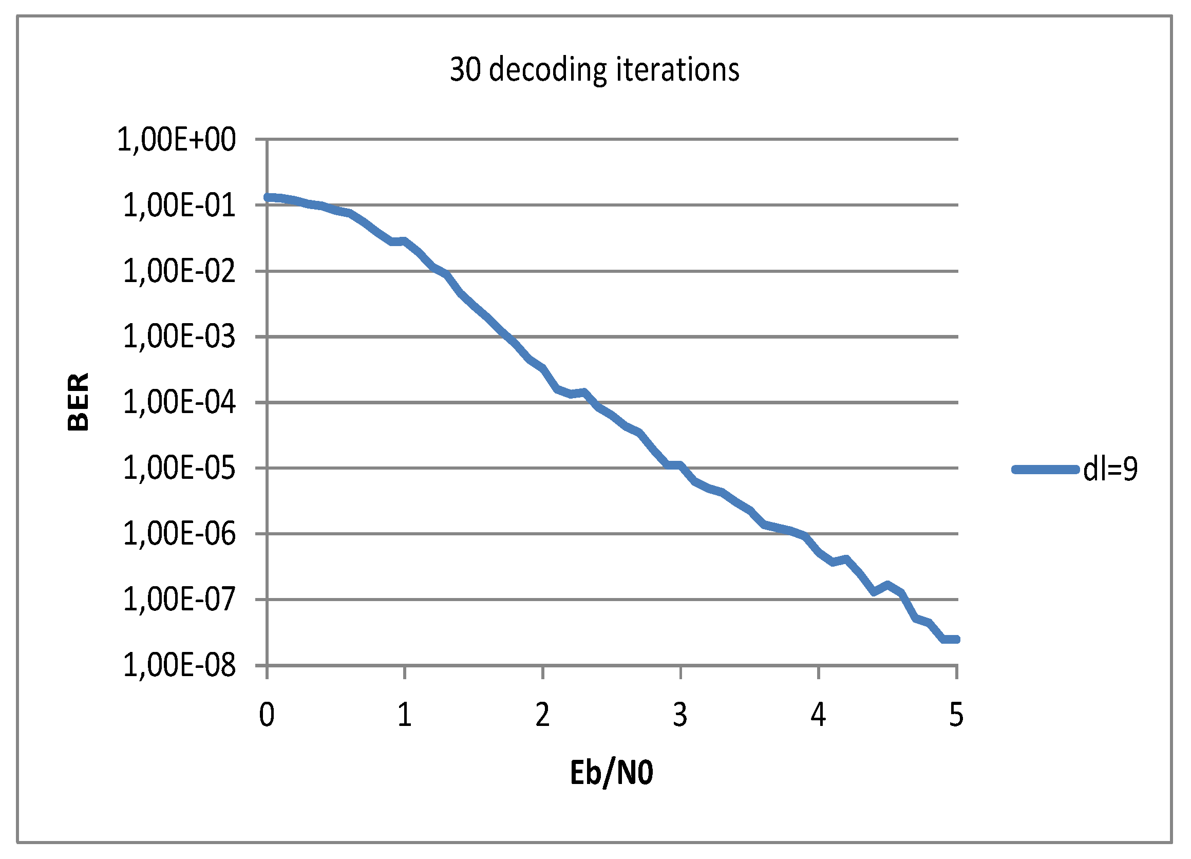
9. Discussion and Simulation Results

Given the pairs $\lambda (x)$ and $\rho (x)$ of Table 1, Table 2, and Table 3, for each of them, an ensemble with a random rate-1/2 LDPC codes has been generated, and their performance simulated using a customized software built on the basis of [22], assuming a memoryless binary input with an additive white Gaussian noise (BI-AWGN) channel.

Since l in Equation (33) is upper bounded by Equation (32), the discussion of the results may be conducted separately for the following two conditions:

• $L_{2}n>(1-r)n$ and
• $L_{2}n<(1-r)n$.

9.1. Case 1: $L_{2}n>(1-r)n$

The rate r of the codes whose pairs $\lambda (x)$ and $\rho (x)$ were listed in Table 1, Table 2, and Table 3, is 1/2. It follows that, for the examples considered in the paper, $1-r=1/2$. Thus, the degree distributions fulfilling the condition $L_{2}n>(1-r)n$ are those with $L_{2}n>n/2$, i.e., $L_2>1/2$. This condition is fulfilled by the distributions having $d_l=4$, 6, and 8 of Table 1. This implicates that $l\le n/2$ for all these codes, i.e., that l is fixed. Given this fixed l value, the performance of the random selected LDPC codes having degree distributions given in the 2-nd, 3-rd, and last column of Table 1, are characterized by an asymptotic BER performance that depends on the probability of Equation (33) only, i.e., only on the value of the product ${\lambda }^{\prime }(0){\rho }^{\prime }(1)$. Taken these three degree distributions, the random selected LDPC code having a pair $\lambda (x)$ and $\rho (x)$ that minimizes Equation (33), and thus is characterized by the best asymptotic BER performance, is the one for which the product ${\lambda }^{\prime }(0){\rho }^{\prime }(1)$ is minimum. This is the case of the code ensemble with $d_l=8$ in Table 1. On the other hand, the random selected LDPC code having a pair $\lambda (x)$ and $\rho (x)$ that maximize Equation (33) is the one for which the product ${\lambda }^{\prime }(0){\rho }^{\prime }(1)$ is the maximum. This is the case of the code ensemble with $d_l=4$ in Table 1. Moreover, the minimization of the product ${\lambda }^{\prime }(0){\rho }^{\prime }(1)$ implies, as expected from Equation (39), the maximization of ${\sigma }_{\mathrm{Jensen}}^{*}$ and, thus, a minimization of ${\mathrm{SNR}}_{\mathrm{gap}}$ and of ${\mathrm{SNR}}_{\mathrm{gap}-\mathrm{spline}}$.

Figure 1 illustrates the BER performances of two randomly generated codes with pairs $\lambda (x)$ and $\rho (x)$ having $d_l=4$ and 8, respectively, minimizing and, respectively, maximizing the product ${\lambda }^{\prime }(0){\rho }^{\prime }(1)$.

As shown in the figure above, the simulated performance achieved by the codes having $d_l=8$ is better than that achieved by the codes having $d_l=4$. For instance, at $E_b/N_0=5$ dB, the BER obtained with $d_l=4$ is ∼3 ×${10}^{-7}$, whereas the BER obtained with $d_l=8$ is ∼5 ×${10}^{-8}$.

9.2. Case 2: $L_{2}n<(1-r)n$

Since, as said above, for the examples considered in the paper, $1-r=1/2$, it follows that the degree distributions fulfilling the condition $L_{2}n<(1-r)n$ are those with $L_{2}n<n/2$, i.e., $L_2<1/2$. This condition is fulfilled by the codes with $d_l=7$ of Table 1, and by all the other codes of Table 2 and Table 3. This implies that $l\le L_{2}n$ for all these codes, i.e., that, given the block length n, l varies with $L_2$. In this case, we expect that a higher upper bound of Equation (32) on the codeword weight l will provide in general a better BER performance. Thus, the dependence of this performance from the product ${\lambda }^{\prime }(0){\rho }^{\prime }(1)$ must be evaluated case by case. For instance, considering Figure 2, Figure 3, and Figure 4, where the performances of three randomly generated codes with pairs $\lambda (x)$ and $\rho (x)$ having $d_l=7$, 9 and 10 are shown respectively, the BER curve obtained with $d_l=7$ (Figure 2) is the worse of the three (at $E_b/N_0=5$ dB the BER is ∼2 × ${10}^{-7}$) and the one obtained with $d_l=9$ (Figure 3) is the best of the three (at $E_b/N_0=5$ dB the BER is ∼2 × ${10}^{-8}$), whereas the one obtained with $d_l=10$ (Figure 4) is intermediate between the above mentioned two (at $E_b/N_0=5$ dB the BER is ∼4 × ${10}^{-8}$) since the code with $d_l=7$ presents the lowest $L_2$ value ($L_2=0.43927$), that with $d_l=9$ presents the highest $L_2$ value ($L_2=0.49128$), whereas the one with $d_l=10$ presents an intermediate $L_2$ value ($L_2=0.46020$) in respect to the other two. As far as the role of the product ${\lambda }^{\prime }(0){\rho }^{\prime }(1)$ is concerned, in this case it may be seen that, even if the code with $d_l=9$ presents a higher value of this product with respect to the code with $d_l=10$ (1.69321 vs. 1.59749), its performance is better (at $E_b/N_0=5$ dB the BER is ∼2 × ${10}^{-8}$) than that of the code with $d_l=10$ (presenting at $E_b/N_0=5$ dB a BER of ∼4 × ${10}^{-8}$) because it presents a higher value of $L_2$.

Thus, in conclusion, the randomly generated code having a degree distribution with $d_l=9$ (Figure 3) is the best since as it has the highest value of $L_2$ (0.49128) even if it presents an intermediate value of the product ${\lambda }^{\prime }(0){\rho }^{\prime }(1)$ (1.69321). Moreover, the code with the lowest value of the product ${\lambda }^{\prime }(0){\rho }^{\prime }(1)$ (1.59749), i.e., the one with $d_l=10$ also presents, as expected from (39), the highest value of ${\sigma }_{\mathrm{Jensen}}^{*}$ (1.03314).

10. Conclusions

The objective of this work was the analysis of the importance of the product ${\lambda }^{\prime }(0){\rho }^{\prime }(1)$ in determining LDPC codes performance, as far as both the weight distribution function and the decoding thresholds are concerned. This analysis was based on [9], as far as the weight distribution function was concerned, and on [10], regarding the LDPC decoding thresholds. The analysis was conducted on two main conditions, i.e., the one for which $L_2>(1-r)$ (being r the code rate) and the one for which $L_2<(1-r)$. In the first case, the role of the product alone was fundamental in determining the performance. In the second, parameter $L_2$ was also important with the product. The best case was that presenting the highest value of $L_2$ together with the lowest value of the product ${\lambda }^{\prime }(0){\rho }^{\prime }(1)>1$. Moreover, a lower value of the product ${\lambda }^{\prime }(0){\rho }^{\prime }(1)$ implied, as expected from (39), a higher value of the upper bound on the decoding threshold ${\sigma }_{\mathrm{Jensen}}^{*}$ and thus, in terms of noise power, a smaller gap from the Shannon limit.

References

1. Gallager, R.G. Low-Density Parity-Check Codes; MIT Press: Cambridge, UK, 1963. [Google Scholar]
2. Tanner, R.M. A recursive approach to low complexity codes. IEEE Trans. Inf. Theory 1981, 5, 533–547. [Google Scholar] [CrossRef] [Green Version]
3. Mackay, D.J.C. Good error correcting codes based on very sparse matrices. IEEE Trans. Inf. Theory 1999, 2, 399–431. [Google Scholar] [CrossRef] [Green Version]
4. Luby, M.G.; Mitzenmacher, M.; Shokrollahi, M.A.; Spielman, D.A. Improved low-density parity-check codes using irregular graphs. IEEE Trans. Inf. Theory 2001, 2, 585–598. [Google Scholar] [CrossRef]
5. Babich, F.; Vatta, F. Turbo Codes Construction for Robust Hybrid Multitransmission Schemes. J. Commun. Softw. Syst. (JCOMSS) 2011, 4, 128–135. [Google Scholar] [CrossRef]
6. Vatta, F.; Soranzo, A.; Comisso, M.; Buttazzoni, G.; Babich, F. Performance Study of a Class of Irregular LDPC Codes through Low Complexity Bounds on Their Belief-Propagation Decoding Thresholds. In Proceedings of the 2019 AEIT International Annual Conference, AEIT’19, Florence, Italy, 18–20 September 2019. [Google Scholar]
7. Babich, F.; Comisso, M. Multi-Packet Communication in Heterogeneous Wireless Networks Adopting Spatial Reuse: Capture Analysis. IEEE Trans. Wirel. Commun. 2013, 10, 5346–5359. [Google Scholar] [CrossRef]
8. Babich, F.; D’Orlando, M.; Vatta, F. Distortion Estimation Algorithms for Real-Time Video Streaming: An Application Scenario. In Proceedings of the 2011 International Conference on Software, Telecommunications and Computer Networks, SoftCOM’11, Split, Croatia, 15–17 September 2011. [Google Scholar]
9. Di, C.; Richardson, T.J.; Urbanke, R. Weight distribution of low-density parity-check codes. IEEE Trans. Inf. Theory 2006, 11, 4839–4855. [Google Scholar] [CrossRef]
10. Vatta, F.; Soranzo, A.; Babich, F. Low-Complexity bound on irregular LDPC belief-propagation decoding thresholds using a Gaussian approximation. Electron. Lett. 2018, 17, 1038–1040. [Google Scholar] [CrossRef] [Green Version]
11. Chung, S.-Y.; Richardson, T.J.; Urbanke, R. Analysis of sum-product decoding of low-density parity-check codes using a Gaussian approximation. IEEE Trans. Inf. Theory 2001, 2, 657–670. [Google Scholar] [CrossRef] [Green Version]
12. Babich, F.; Noschese, M.; Soranzo, A.; Vatta, F. Low complexity rate compatible puncturing patterns design for LDPC codes. In Proceedings of the 2017 International Conference on Software, Telecommunications and Computer Networks, SoftCOM’17, Split, Croatia, 21–23 September 2017. [Google Scholar]
13. Babich, F.; Noschese, M.; Vatta, F. Analysis and design of rate compatible LDPC codes. In Proceedings of the 27th IEEE International Symposium on Personal, Indoor and Mobile Radio Communications, PIMRC ’16, Valencia, Spain, 4–8 September 2016. [Google Scholar]
14. Tan, B.S.; Li, K.H.; Teh, K.C. Bit-error rate analysis of low-density parity-check codes with generalised selection combining over a Rayleigh-fading channel using Gaussian approximation. IET Commun. 2012, 1, 90–96. [Google Scholar] [CrossRef]
15. Chen, X.; Lau, F.C.M. Optimization of LDPC codes with deterministic UEP properties. IET Commun. 2011, 11, 1560–1565. [Google Scholar] [CrossRef]
16. Babich, F.; Soranzo, A.; Vatta, F. Useful mathematical tools for capacity approaching codes design. IEEE Commun. Lett. 2017, 9, 1949–1952. [Google Scholar] [CrossRef]
17. Vatta, F.; Babich, F.; Ellero, F.; Noschese, M.; Buttazzoni, G.; Comisso, M. Performance study of a class of irregular LDPC codes based on their weight distribution analysis. In Proceedings of the 2019 International Conference on Software, Telecommunications and Computer Networks, SoftCOM’19, Split, Croatia, 19–21 September 2019. [Google Scholar]
18. Richardson, T.J.; Shokrollahi, A.; Urbanke, R. Design of capacity- approaching irregular low-density parity-check codes. IEEE Trans. Inf. Theory 2001, 2, 619–637. [Google Scholar] [CrossRef] [Green Version]
19. Vatta, F.; Soranzo, A.; Comisso, M.; Buttazzoni, G.; Babich, F. New explicitly invertible approximation of the function involved in LDPC codes density evolution analysis using a Gaussian approximation. Electron. Lett. 2019, 22, 1183–1186. [Google Scholar] [CrossRef]
20. Vatta, F.; Soranzo, A.; Babich, F. More accurate analysis of sum-product decoding of LDPC codes using a Gaussian approximation. IEEE Commun. Lett. 2019, 2, 230–233. [Google Scholar] [CrossRef] [Green Version]
21. Chung, S.-Y. On the Construction of Some Capacity-Approaching Coding Schemes. Ph.D. Thesis, MIT, Cambridge, MA, USA, 2000. Available online: http://dspace.mit.edu/handle/1721.1/8981 (accessed on 9 December 2019).
22. Boscolo, A.; Vatta, F.; Armani, F.; Viviani, E.; Salvalaggio, D. Physical AWGN channel emulator for Bit Error Rate test of digital baseband communication. Appl. Mech. Mater. 2013, 241–244, 2491–2495. [Google Scholar] [CrossRef]
Figure 1. BER with respect to E b / N 0 in dB with d l = 4 and d l = 8 , n = 1000 , and iterations number I = 50 .
Electronics 08 01515 g001
Figure 2. BER with respect to E b / N 0 in dB with d l = 7 , n = 1000 , and iterations number I = 30 .
Electronics 08 01515 g002
Figure 3. BER with respect to E b / N 0 in dB with d l = 9 , n = 1000 , and iterations number I = 30 .
Electronics 08 01515 g003
Figure 4. BER with respect to E b / N 0 in dB with d l = 10 , n = 1000 , and iterations number I = 30 .
Electronics 08 01515 g004