Salp Swarm Optimization Algorithm-Based Fractional Order PID Controller for Dynamic Response and Stability Enhancement of an Automatic Voltage Regulator System

Abstract

Owing to the superior transient and steady-state performance of the fractional-order proportional-integral-derivative (FOPID) controller over its conventional counterpart, this paper exploited its application in an automatic voltage regulator (AVR) system. Since the FOPID controller contains two more control parameters (µ and $\lambda$) as compared to the conventional PID controller, its tuning process was comparatively more complex. Thus, the intelligence of one of the most recently developed metaheuristic algorithms, called the salp swarm optimization algorithm (SSA), was utilized to select the optimized parameters of the FOPID controller in order to achieve the optimal dynamic response and enhanced stability of the studied AVR system. To validate the effectiveness of the proposed method, its performance was compared with that of the recently used tuning methods for the same system configuration and operating conditions. Furthermore, a stability analysis was carried out using pole-zero and bode stability criteria. Finally, in order to check the robustness of the developed system against the system parameter variations, a robustness analysis of the developed system was undertaken. The results show that the proposed SSA-based FOPID tuning method for the AVR system outperformed its conventional counterparts in terms of dynamic response and stability measures.

1. Introduction

Maintaining consistent and stable voltage levels in a power system requires proper control management of power networks. A nominal deviation in voltage from expected ratings may cause a severe decline in the performance of the connected equipment. Surges in the terminal voltage fluctuate reactive power by a large margin and may cause the power system to reach an unstable level of operation. Additionally, this may lead to increased losses in power lines and unbalanced voltage fluctuations which directly affect the real and reactive power flow. A classical solution to voltage fluctuations on the power generation side is the usage of an automatic voltage regulator (AVR) that controls the voltage levels by maintaining the voltage of an alternator at a specified level. Therefore, the performance of power systems is highly subjected to the stability of AVR. A general structure of the voltage control through AVR is depicted in Figure 1.

As shown in Figure 1, the AVR controller compares the generator output terminal voltage with the set reference voltage, and, as per the error signal, it changes the field excitation of the generator to maintain constant terminal voltage. However, the fast-stabilized response of the regulator is highly dependent on the generator field windings (loaded with high inductance) and load variations. Therefore, there is a need to improve AVR performance to encounter high inductance and changes in load variation for strong retaliation to continuous surges in terminal voltage. Recently, researchers have proposed several control strategies to improve AVR stability and its capability to control terminal voltage efficiently with a suitable dynamic response. Following improvements in control strategies, PID (proportional-integral-derivative) controller is proven to be one of the most effective controllers in stabilizing the terminal voltage with a robust response and simple design [1]. However, due to the increasing load and, hence, the switching operation, more precise control is required in order to enhance the steady-state and dynamic performance of the power system. For the mentioned reasons, a conventional PID controller was replaced by the fractional order PID (FOPID) controller in an AVR system for the very first time in 2007 by Karimi et al. [2]. The mentioned study proved the superiority of the FOPID controller over its conventional counterpart in almost all the key steady-state and dynamic response indicators. The key reason for FOPID performance superiority is that it has more tuning freedom due to the greater number of tuning parameters, which helps in stabilizing the plant under control, and offers improvements in control loop robustness [3]. The FOPID controller was designed by Podlubny [4] in 1999. In addition to the three common tuning parameters (K_P, K_I, K_D) of the conventional PID controller, the FOPID controller possesses two additional control parameters, i.e., the order of fractional integration ($\lambda$) and order of fractional derivative (µ). These additional parameters in FOPID provide increased control flexibility and an added advantage of tuning the control system using respective error information at the cost of complex control strategies.

However, due to the presence of two additional parameters, tuning of the FOPID controller is relatively more complex and tedious as compared to that of the PID controller. With the advancement in the soft-computational techniques, the solution of the mentioned problem has been attempted by many researchers around the world using different artificial intelligence-based optimization techniques such as particle swarm optimization (PSO) [5,6,7], simulated annealing (SA) [8], genetic algorithm (GA) [9], and a few improved versions [10]. Despite their superior performance over the traditional methods of FOPID tuning, all the mentioned optimization algorithms are bound with major drawbacks. For example, the localized solutions by GA restrict its usage to static data sets [11,12]. The PSO suffers from high uncertainty in its parameter selection and suffers local optimum stagnation for high dimensional search spaces [13]. This necessitates the modern FOPID-based AVR controller to be tuned by a modern and intelligent algorithm in order to optimize its dynamic response, stability, and robustness. This fact drove this dissertation to further explore the optimization algorithms for a better solution to FOPID-based AVR systems.

This research work explored the application of a swarm intelligence-based FOPID controller in AVR systems. For the very first time in the literature, to the best of the authors’ knowledge, the SSA was utilized to optimally tune the FOPID parameters for optimizing the dynamic response, robustness, and stability of the studied system. The proposed method utilizes the intelligence of SSA to minimize an error integrating the fitness function in order to attain optimal control parameters (K_P, K_I, K_D, $\lambda ,$ and µ) for a PI^ʎD^µ controller. The obtained optimized parameters ensure the optimal dynamic response of the AVR system with reduced settling time and overshoot as compared to traditional methods utilized in recent literature. Furthermore, the effectiveness of the proposed method is reported along with a comparative analysis with differential evolution (DE) [14], the particle swarm optimization algorithm (PSO) [15], artificial bee colony (ABC) [14], the grasshopper optimization algorithm (GOA) [16], the bibliography-based optimization (BBO) [17] algorithm, and the pattern search algorithm (PSA) [18]. The results prove the superiority of the proposed method over all the studied methods under an identical system configuration and operating conditions.

The remainder of this paper is organized as follows: Section 2 presents the mathematical foundation of the AVR system along with the FOPID controller. Section 3 is dedicated to the proposed SSA basics and its optimizing features. Additionally, the fitness function formulation and its justification are explained in Section 4. A comparative analysis along with the effectiveness of the proposed algorithm is reported in the results, Section 5. Lastly, Section 6 concludes the current research work with proposed future directions.

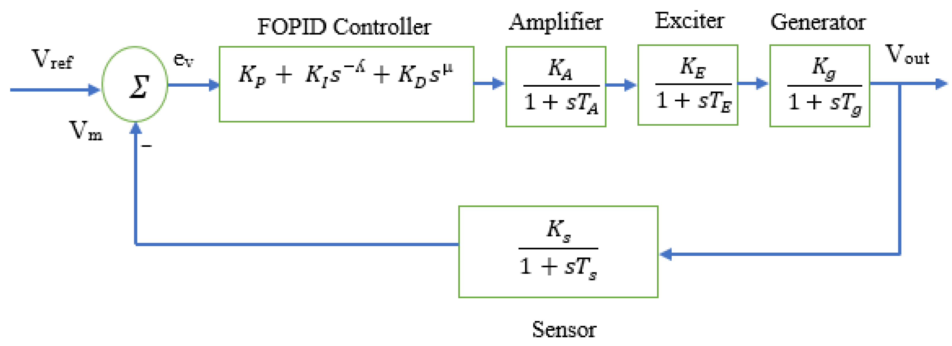
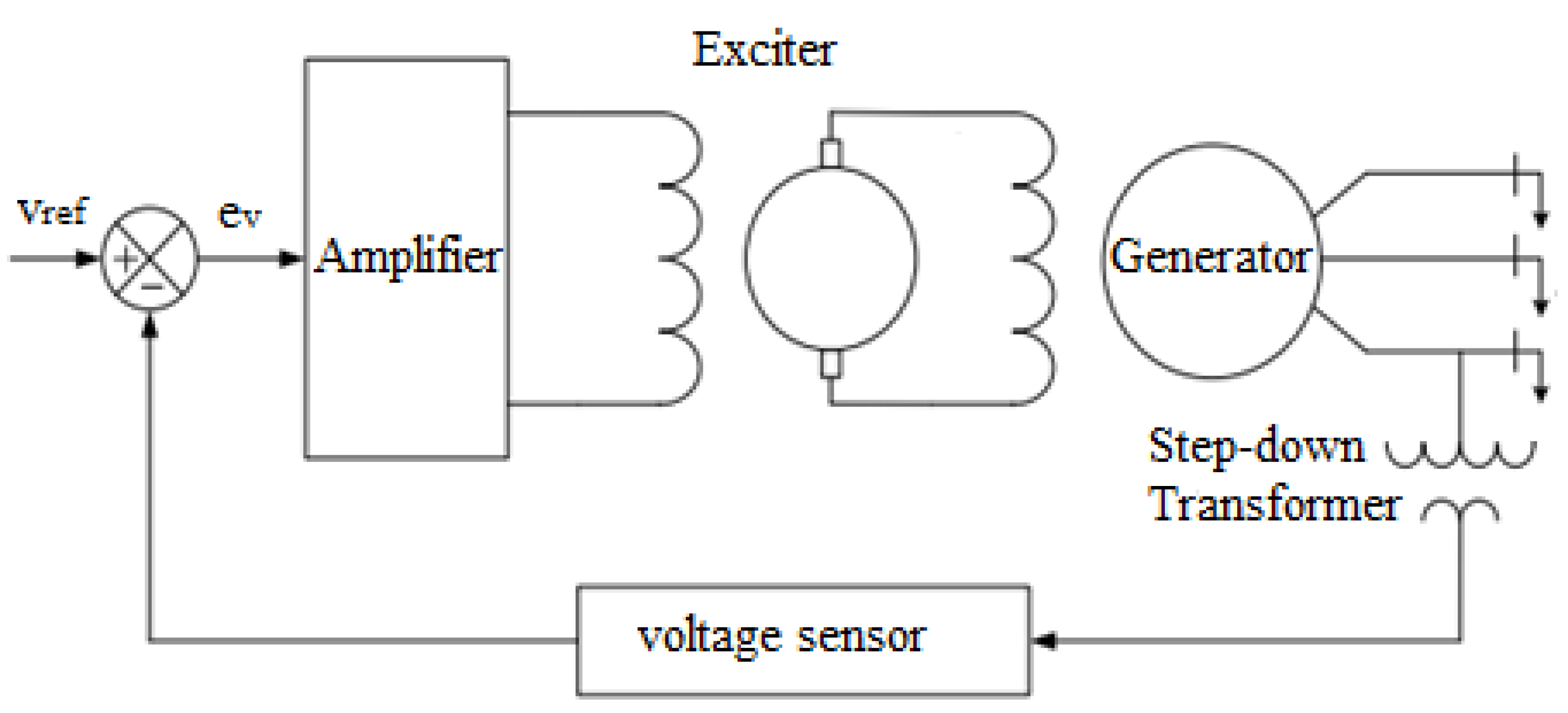
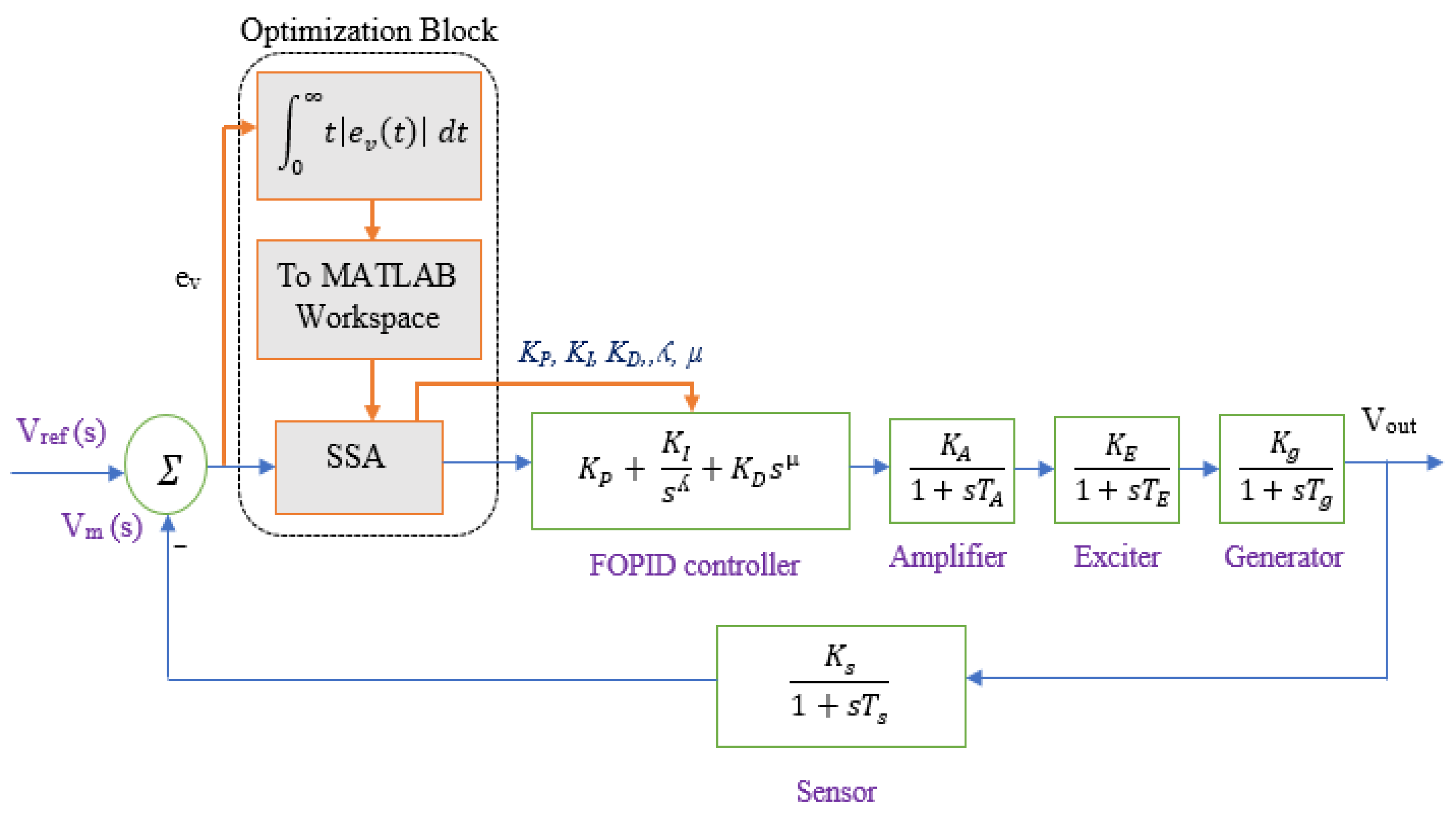
2. Mathematical Modelling of AVR System

Inevitable surges in terminal voltage are the major cause of power system performance degradation. One of the easiest and most common solutions to avoid the mentioned problem is to use an AVR system at the terminals of a synchronous generator. An AVR performs as a feedback control system that receives the feedback signal from potential and current transformers placed at the output terminals of the generator. The potential transformer continuously observes the voltage variations in the alternator, while the current transformer feeds the current signal to the controller circuit. The potential transformer feeds a comparator to calculate the error by comparing its output voltage value with the reference or nominal voltage, and the resulted signal (voltage error) is fed to the field windings of an alternator after due amplification. Moreover, an exciter is employed in order to bridge the comparator and field windings. Generally, the AVR system is composed of four basic components: sensor, amplifier, exciter, and generator. This research paper used a linear mathematical model for each basic component of the AVR. A block diagram of the FOPID-based AVR system with all the major components is shown in Figure 2.

Where ${\mathrm{V}}_{\mathrm{ref}}$ is the reference voltage, while ${\mathrm{V}}_{\mathrm{m}}$ represents the measured output voltage value of the sensor. A linear model of the amplifier results as a combination of gain and the time constant in the transfer function is given in Equation (1) [19].

$$G_{amp}\left(s\right) = \frac{K_A}{1+S{T}_A}$$

(1)

where K_A represents the gain of the amplifier with a value ranging from 10 to 40, and T_A represents the time constant of the amplifier whose value ranges from 0.02 s to 0.1 s. Similarly, Equation (2) mathematically models the transfer function of an exciter employed in AVR [19].

$$G_{exc}\left(s\right) = \frac{K_E}{1+S{T}_E}$$

(2)

In Equation (2), K_E represents the gain ranging from 1 to 10, and T_E represents the time constant in the exciter model ranging from 0.4 s to 1.0 s. Moreover, a transfer function of the terminal voltage with the field voltage of the generator is modeled by Equation (3) [19].

$$G_{gen}\left(s\right) = \frac{K_G}{1+S{T}_G}$$

(3)

where K_G represents the generator gain with a range from 0.7 to 1.0, and T_G represents the time constant in the generator transfer function. The time constant can attain a minimum value of 1 s reaching up to 2.0 s. Equation (4) presents the transfer function for the sensor connected as a feedback loop of the AVR block diagram as shown in Figure 2 [19].

$$G_{sen}\left(s\right) = \frac{K_S}{1+S{T}_S}$$

(4)

In Equation (4), K_S represents the sensor gain ranging from 0.9 to 1.1, and T_S represents the time constant ranging from 0.001 s to 0.06 s. Finally, Equation (5) represents the transfer function model for the FOPID controller.

$$G_{fopid}\left(s\right) = K_P+ K_I{s}^{-ʎ}+K_D{s}^{\mu }$$

(5)

where V_ref is the reference or rated voltage of the system, while V_m and V_out represent the measured and output voltage of AVR, respectively. Equation (6) represents the overall FOPID controller transfer function G(s) for an AVR system.

$$G\left(s\right) = \frac{G_{fopid}\left(s\right).G_{amp}\left(s\right).G_{exc}\left(s\right).G_{gen}\left(s\right)}{1+ G_{fopid}\left(s\right).G_{amp}\left(s\right).G_{exc}\left(s\right).G_{gen}\left(s\right).G_{sen}\left(s\right)}$$

(6)

It is worthwhile to mention that one of the major advantages of the conventional PID controller is that it can be easily converted into a PI or PD controller based on the requirement and control objectives. For example, the authors in Reference [20] utilized a PI controller to control the DC bus voltage in a hybrid AC/DC microgrid. In another study [21], the authors used the same controller in voltage and current control loops to regulate bus voltage and current in a hybrid renewable nano-grid. Similarly, it is also possible in FOPID control action which may operate as PI or PD or FOPI or FOPID without one of the fractional-order tuning variables, hence providing greater flexibility in control action as compared to its conventional counterpart. Furthermore, due to the two additional fractional order parameters in FOPID-based control action, finer control can be obtained which, in turn, provides higher controllability as compared to the conventional PID controller.

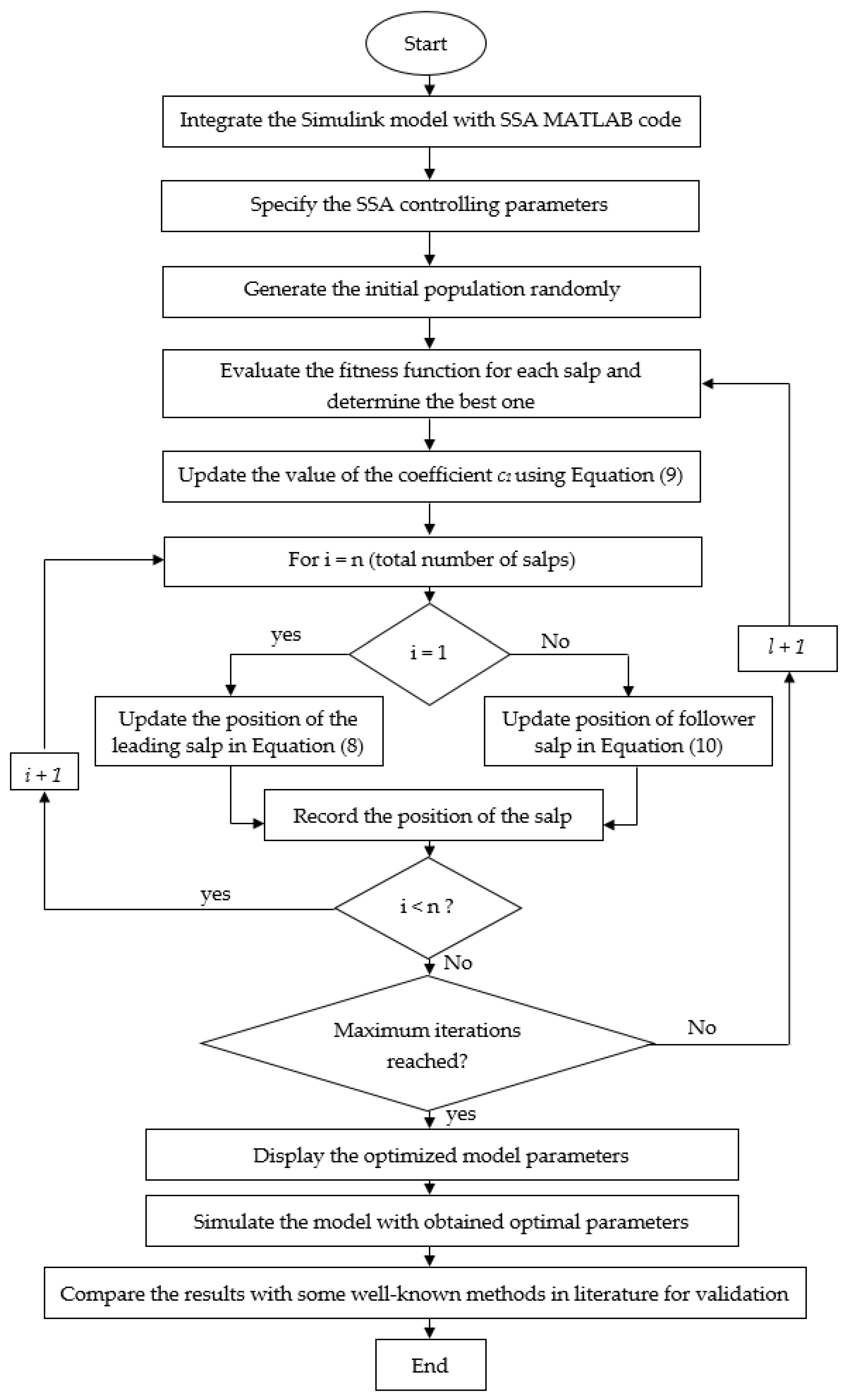
3. Salp Swarm Optimization Algorithm and Its Implementation in the Current Study

This section presents the motivational factors for the proposed optimization algorithm along with its mathematical model. A transparent bodied salp is a vertebrate and is famous for making spiral chains during its movement. Salps are usually quoted for their propulsion nature in water like a jet. To mathematically model the swarming of salps, the random initialization salp positions is made as depicted in Equation (7) [22].

$${\mathit{K}}_{\mathbf{1}}^{\mathbf{1}:\mathit{n}} = \mathit{r}\mathit{a}\mathit{n}\mathit{d}(\dots )(\mathit{u}{\mathit{b}}_{\mathit{j}}-\mathit{l}{\mathit{b}}_{\mathit{j}})+\mathit{l}{\mathit{b}}_{\mathit{j}},\forall \mathit{j} \in \mathit{n}\mathit{o}.\mathit{o}\mathit{f} \mathit{v}\mathit{a}\mathit{r}\mathit{i}\mathit{a}\mathit{b}\mathit{l}\mathit{e}\mathit{s}$$

(7)

where $K_1^{1:n}$ shows the initial positions of the salps$, u{b}_j$ indicates the upper limit, and $l{b}_j$ represents the lower limit. Furthermore, rand (….) is the mathematical notation used for the generation of a random number between 0 and 1.

Secondly, to imitate the salp swarm mechanism, a group leader and followers need to be decided. A salp individual who is leading the whole swarm is considered the leader, while the rest of the salps are considered as followers. In this formation, the leader is responsible for guiding the group towards a safer position with its every successive move. Equation (8) represents the mathematically translated version of the leader in salp swarm, where M represents the target food and K represents the two-dimensional position of each Salp [22]:

$${\mathit{K}}_{\mathit{j}}^{\mathbf{1}} = \{\begin{array}{l}{\mathit{M}}_{\mathit{i}}+{\mathit{c}}_{\mathbf{1}}\left(\right(\mathit{u}{\mathit{b}}_{\mathit{j}}-\mathit{l}{\mathit{b}}_{\mathit{j}}){\mathit{c}}_{\mathbf{2}}+\mathit{l}{\mathit{b}}_{\mathit{j}}){\mathit{c}}_{\mathbf{3}}\ge \mathbf{0}\\ {\mathit{M}}_{\mathit{i}}-{\mathit{c}}_{\mathbf{1}}\left(\right(\mathit{u}{\mathit{b}}_{\mathit{j}}-\mathit{l}{\mathit{b}}_{\mathit{j}}){\mathit{c}}_{\mathbf{2}}+\mathit{l}{\mathit{b}}_{\mathit{j}}){\mathit{c}}_{\mathbf{3}}<\mathbf{0}\end{array}$$

(8)

$K_j^1$ shows the position of the leader, $M_i$ is the position of the target food in the $j_{th}$ dimension, $u{b}_j$ indicates the upper limit of $j_{th}$ dimension, $l{b}_j$ indicates the lower limit of $j_{th}$ dimension, and c₁, c₂, and c₃ are random numbers. The SSA represents a long chain consisting of salps; therefore, this type of algorithm can circumvent the localized maximum or minimum solutions. Equation (9) represents the food perusing process of the leading salp by equating its movement towards the target food. This is one of the important parameters of SSA that guides the follower salps for catching food sources effectively.

$${\mathit{c}}_{\mathbf{1}} = \mathbf{2}{\mathit{e}}^{-{\left(\frac{\mathbf{4}\mathit{l}}{\mathit{L}}\right)}^{\mathbf{2}}}$$

(9)

where l/L represents the ratio of the current iteration to the maximum intended iterations of the salp swarm. Moreover, random approximations in the range of 0 to 1 are assigned to $c_2$ and $c_3$; this approximation is responsible for the direction of the subsequent position for every j^th dimension depending upon the step size. Newton’s law of motion plays its role in determining the subsequent positions of the followers as shown in the Equation (10).

$${\mathit{K}}_{\mathit{j}}^{\mathit{i}} = \frac{\mathbf{1}}{\mathbf{2}} \mathit{a}{\mathit{t}}^{\mathbf{2}}+{\mathit{v}}_{\mathbf{0} }\mathit{t}$$

(10)

where i ≥ 2 and $K_j^i$ represents the position of the followers. The above expression represents the direction in the j^th dimension for any follower specified by the superscript of K. In Equation (1), t represents the time and ${\mathit{v}}_{\mathbf{0}}$ is the initial velocity of the salp follower which is assumed to be zero. Usually, time is represented by the iteration number in the optimization analysis; therefore, a step size of 1 was chosen for the time variable. A simplified version of Equation (10) is shown in Equation (11).

$${\mathit{K}}_{\mathit{j}}^{\mathit{i}} = \frac{{\mathit{K}}_{\mathit{j}}^{\mathit{i}}+ {\mathit{K}}_{\mathit{j}}^{\mathit{i}-\mathbf{1}}}{\mathbf{2}}$$

(11)

It is important to note that the salp chain possesses the potential of moving towards the continuously changing global optimum (food source) in order to find a better solution by exploring and exploiting the defined search space. Some of the very important features of SSA which make it different from the conventional optimization algorithms are listed as follows [22]:

• The algorithm keeps the best-obtained solution after each iteration and assigns it to the global optimum (food source) variable. Hence, it can never be wiped out even if the whole population deteriorates;
• The SSA updates the position of the leading salp with respect to the food source only which is the best solution obtained so far; therefore, the leader salp always explores and exploits the space around it for a better solution;
• The SSA updates the position of follower salps with respect to each other in order to let them move towards the leading salp gradually;
• Gradual movements of follower salps prevent the SSA from easily stagnating into local optima;
• Parameter c₁ is decreased adaptively over the course of iterations which helps the algorithm to explore the search space at starting and exploits it at the ending phase;
• The SSA has only one main controlling parameter (c₁) which reduces the complexity and makes it easy to implement.

The abovementioned merits of the SSA make it potentially able to solve the optimization problems better than conventional optimization methods and, hence, became the motivation for the current research work. In addition, the adaptive mechanism of SSA allows this algorithm to find an accurate estimation of the best solution by continuously avoiding becoming trapped in local solutions. The overall procedure of the SSA in association with the FOPID controller parameter optimization for the AVR system is depicted in the flowchart shown in Figure 3.

Figure 3 describes the optimization mechanism of SSA for solving the current optimization problem. The SSA randomly spread all search agents (salps) over the defined search space. Then, it assesses the current population of salps to detect the leading salp and make all other salps follow the leader. In this process, the variable c₁ is updated by Equation (9). The rule in Equation (8) helps the SSA inform the state of the leader, while Equation (10) changes the position of the follower salps accordingly. Until satisfying the stopping condition, all steps excluding the initialization phase will be repeated to upsurge the quality of salps as much as possible. Since the FOPID gains are adopted as the optimization variables in the developed AVR model, the algorithm tries to minimize an error integrating fitness function (FF) in order to achieve optimal values of mentioned parameters which consequently led to the optimized dynamic response of the studied system as validated by the results of this study.

The literature studied shows that the optimization capability of SSA is relatively higher when performance metrics are based on convergence time and solution quality. Moreover, exploration and exploitation balance by the swarming mechanism provides the SSA with a higher hand on alternative metaheuristic search algorithms. The reported capabilities of the SSA has attracted many researchers in the field of PV module parameter identification [23], optimal allocation and capacity of DGs [24], fuel cell optimal parameter extraction [25], Artificial Neural Network (ANN) training for pattern recognition [26] and load frequency control [27]. These verified capabilities of the searching mechanism of the SSA are a major motivation for FOPID parameter optimization using the mentioned algorithm.

4. Fitness Function Formulation and Implementation

The solution to most of the optimization problems is conditional to the formulation of the FF. The fitness function is described as the mathematical expression of system variables that need to be minimized or maximized during the optimization process in order to attain the optimal response of the system under study. Since the least voltage error is required for an AVR system, the minimization of an error integrating expression has been adopted as the FF for the current research work. The minimization of error increases the proximity of the optimized parametric solutions for the tuning of the PID/FOPID controller. The most widely used error integrating fitness functions in literature are the integral absolute error (IAE), integral squared error (ISE), integral time-weighted squared error (ITSE), and integral time absolute error (ITAE). The ITAE is the most widely used error integrating fitness function referred to in the literature due to the fact of its smoother employment and better outcomes as compared to other contenders like ISE, IAE, and ITSE [28,29]. Both ISE and ITSE are very violent criterions due to the squaring of error and, hence, produce impractical results. Further, compared to ITAE, IAE is also an inadequate choice, owing to the integration of the time multiplying error function, providing more realistic error indexing [30]. Therefore, the proposed algorithm uses ITAE as the fitness function to optimize the studied system’s response. A mathematical representation of ITAE is expressed in Equation (12).

$$ITAE ={\int }_0^{\infty }t\left|e_v\left(t\right)\right|dt$$

(12)

where t represents the time of simulation and e_v(t) represents the error signal which is calculated by subtracting the sensor’s output voltage from the reference voltage as given in Equation (13).

$$e_v = V_{ref}-V_m$$

(13)

It is worthwhile to mention that the formulated FF was designed in SIMULINK, while the SSA was coded in the MATLAB editor window. The current value of the FF was transported to the MATLAB workspace using the “TO WORKSPACE” block which was then evaluated by the SSA code for exploring the optimal values of the FOPID controller through the optimization process mentioned in Figure 3. The resulting block diagram for the proposed FOPID optimization in the AVR system by the SSA is depicted in the simplest way in Figure 4.

It is worth mentioning that the minimization of ITAE as a fitness function is very crucial for achieving optimized parameters for FOPID controllers (K_P, K_I, K_D, µ, and $\lambda$). If the optimization algorithm gets stuck in a local solution, the consequences are reflected in the transient response of the system. Consequently, the system will observe large overshoots and settling time before settling to its final steady-state value. In the worst-case scenario, the system may step-into an unstable region of its operation and can cause supply interruption or damage of equipment due to the unstable voltage supply. Therefore, in order to avoid the mentioned issue, the current study attempts to explore an offline optimization method for selecting the optimal FOPID gains which are suitable for the optimal operation of the AVR and, hence, complete power system. The high-level programming in MATLAB was used to implement the SSA’s initializations and execution. The optimized parameters from the MATLAB workspace were imported to the SIMULINK FOPID-AVR model in order to have a comparative view of the system’s transient response.

5. Results and Discussion

In order to analyze the effectiveness of the proposed SSA algorithm along with its implementation in an FOPID-based AVR system, MATLAB/SIMULINK (2018a) was employed in a 2.77 GHz, Intel Core™ i7 computer. A maximum number of iterations was set as 50 for the SSA and its competitor algorithm. Since the random nature of SSA demands multiple simulation runs of the data set, therefore, in this research work, a simulation run of 20 times was averaged in order to get the final optimized values. In order to obtain the corresponding response of the studied system with the proposed method, the FOPID parameters were injected into the SIMULINK model and the corresponding voltage response was analyzed for different operating conditions of the AVR system. The obtained results are presented and discussed in the subsequent subsections.

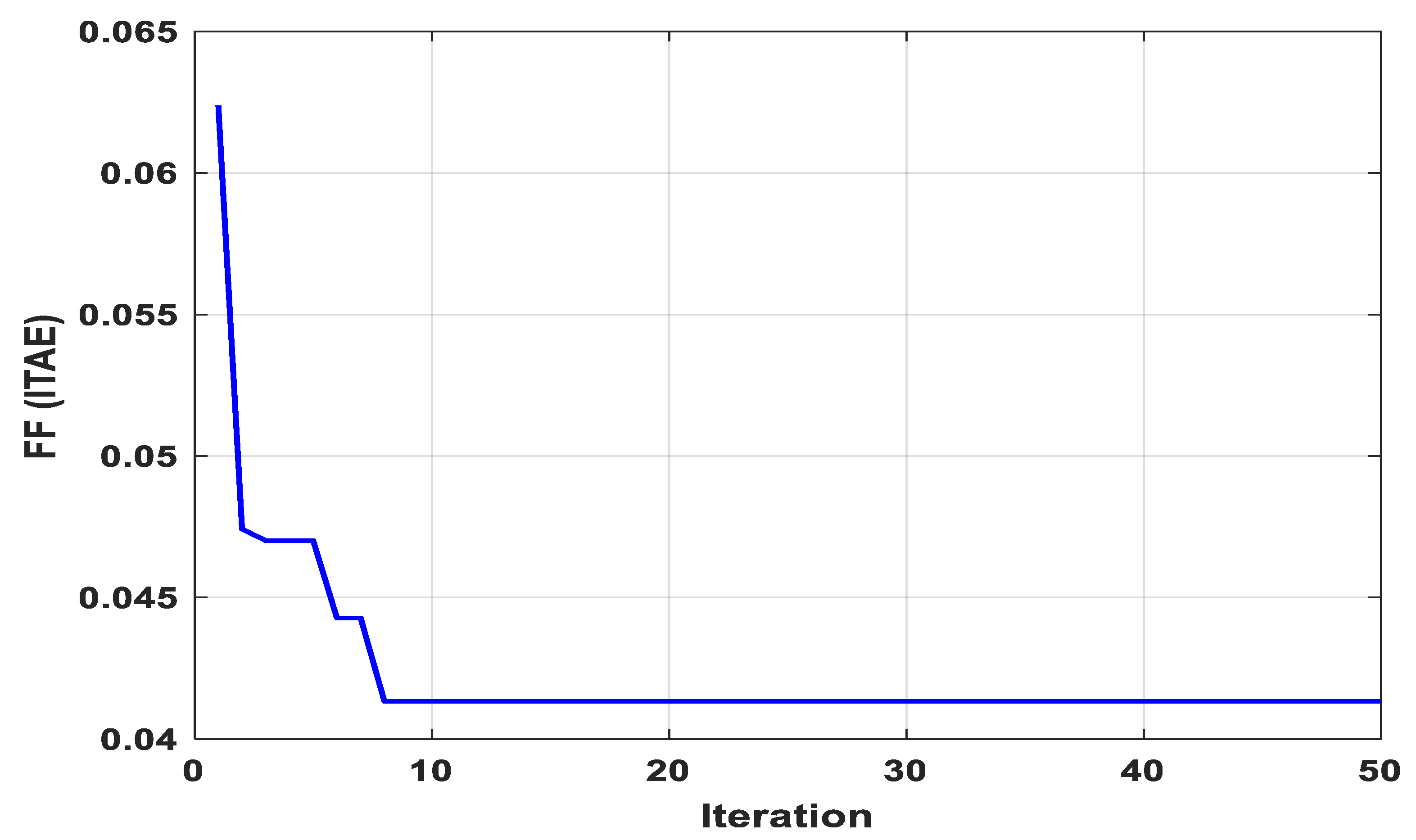
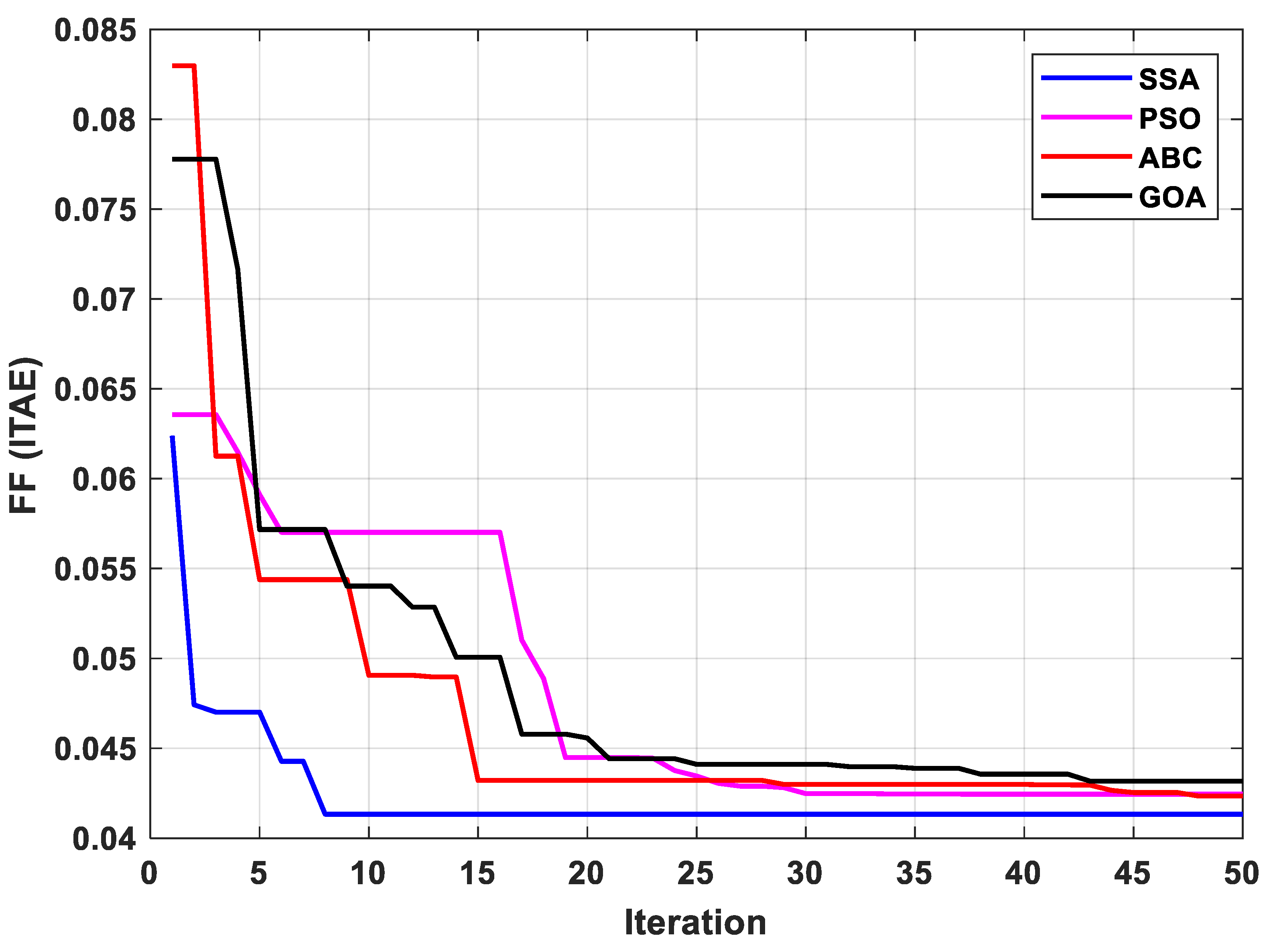
5.1. SSA Convergence Behavior

Figure 5 shows the convergence behavior of the proposed SSA in solving the current optimization problem for obtaining optimal FOPID parameters. It is observable that the value of ITAE dropped with an increase in the number of iterations. Moreover, ITAE represents the fitness function; therefore, the minimization of ITAE ensures advancements towards optimal vicinity.

For any convergence curve in the optimization process, two of the most important parameters to be assessed are the convergence rate and ultimate minimized or maximized value of FF. The first quantity decides what will be the speed of the convergence curve, while the second quantity provides direct information about the quality of the solution achieved by the optimization algorithm [12]. It is quite clear in Figure 5 that the SSA optimization technique achieves a suitable solution in minimizing the stated FF with higher solution quality and convergence rate. The minimized value for the FF for the complete minimization process is 0.004195 and is obtained in the 8th iteration of the simulation. Furthermore, to fairly evaluate the solution quality and convergence rate of the proposed SSA-based FOPID tuning method, its performance was compared with some of the well-known optimization algorithms with identical FF (ITAE) and optimization parameters like the number of search agents, iterations, and search space boundaries. The outcomes are presented in Figure 6.

It is obvious from Figure 6 that the SSA-based FOPID tuning method provided a better convergence rate and quality of solution as compared to the PSO-, ABC-, and GOA-based methods for the identical system and optimization parameters. It is worthwhile to mention that, in order to commence a fair comparison among the studied algorithms, they were made to optimize the given FF under identical iteration numbers, i.e., search agents: 50; number of dimensions: 5. Since all the studied algorithms are based on random number generation during their initial phase and are stochastic in nature, each algorithm was run 10 times to optimize the identical FF. As the objective of the study was to minimize the formulated FF, its least value for each algorithm was adopted and presented in Figure 6. Furthermore, the number of iterations was set at 50 in this case using the “trial and error” method based on a survey of the literature. Further increasing the number of iterations might have given a further reduced value of FF; however, the time for the optimization process would have been large which is one of the important factors that needs to be considered for the optimization process. It can be concluded from Figure 6 that all the studied optimization algorithms reached their minimum value well before the set iteration number.

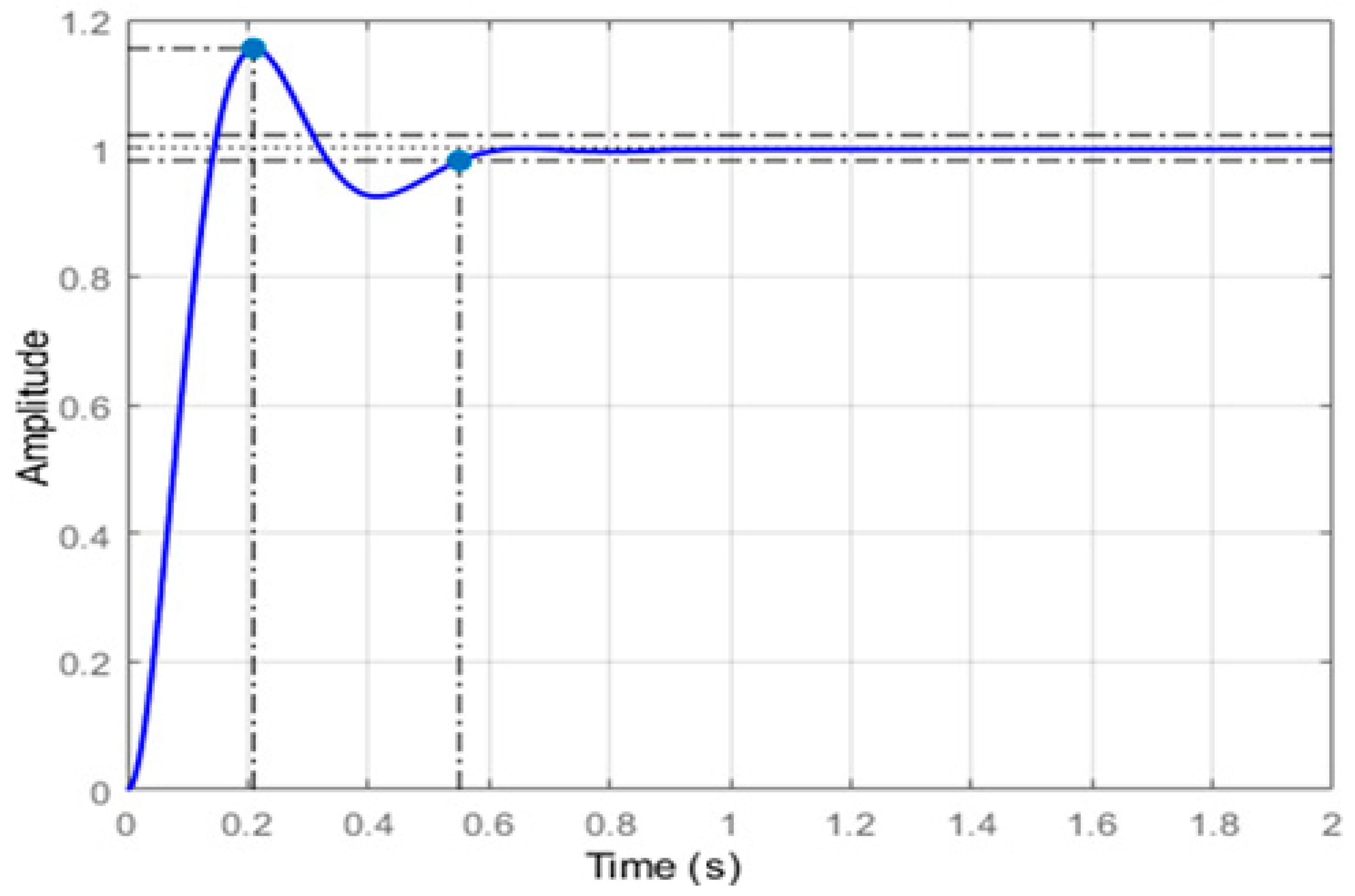
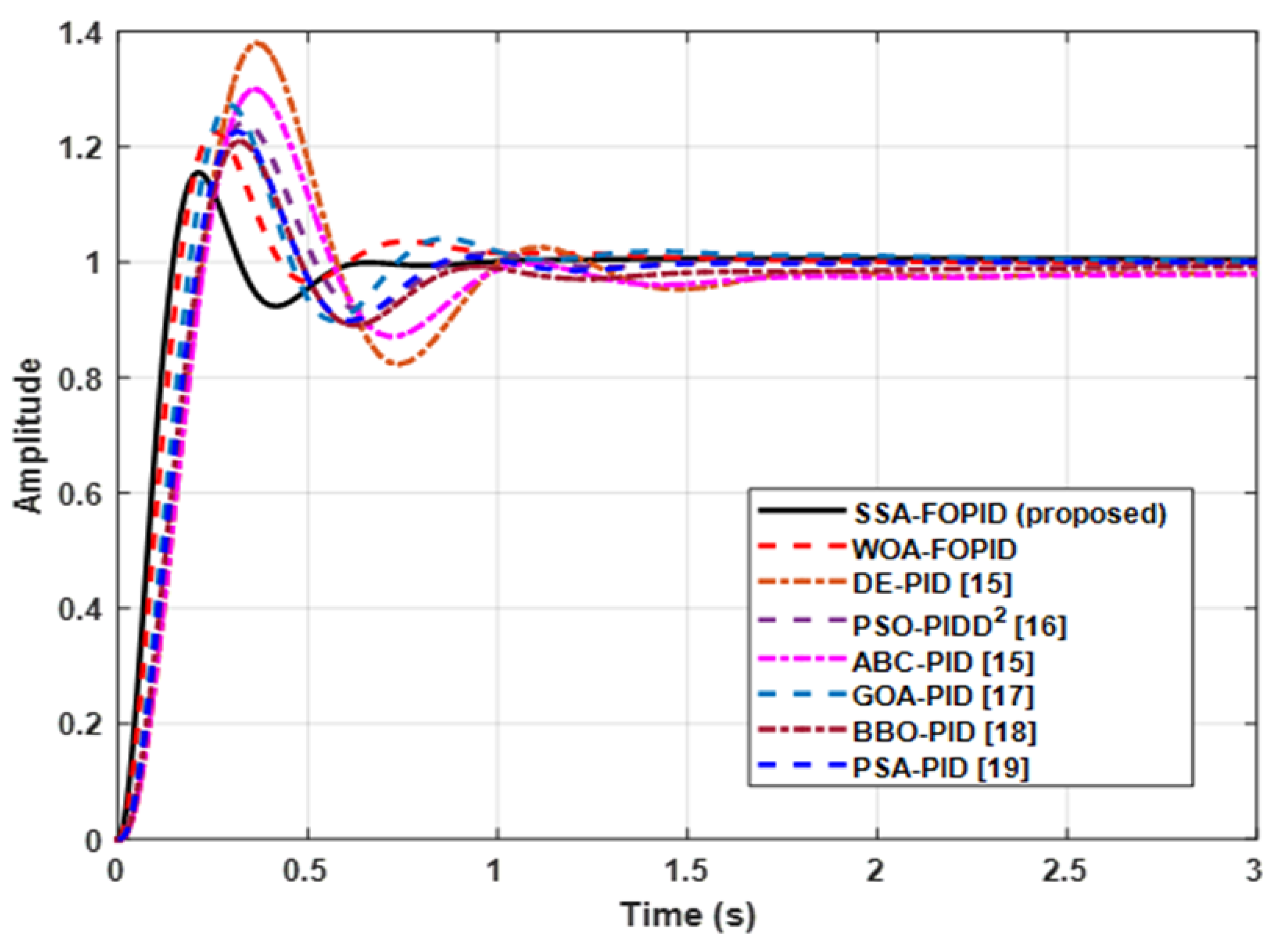
5.2. Transient Response Analysis

The optimized gains of the PID controller obtained at the end of the simulation are given as K_P = 1.99820165729046, K_I = 1.17065053226562, K_D = 0.574968449143989, $\lambda$ = 1.13952046907660, and µ = 1.16565794054897. By rounding-off and inserting the obtained FOPID parameters and other time constant and gain values into Equation (6), the overall transfer function model of the studied AVR system is depicted in Equation (14).

$$\frac{v_{out}\left(s\right)}{v_{ref}\left(s\right)} = \frac{0.575s^{2.3}+1.998s^{1.14}+1.171}{s^{1.14}}$$

(14)

The overall transfer function model was then energized by a unit step input signal to assess the transient response characteristics of the AVR system at stake. Figure 7 shows the voltage magnitude for the unit step input to the studied AVR system.

In this research work, rise time, settling time, peak time, and maximum overshoot were chosen as the performance metrics for characterization of the transient response for a unit step input. The settling time was referred to as the time required to reach 2% of the final steady-state value, while the time required for the response to rise from 10% to 90% of its final value was referred to as the rise time. To highlight the advantages of the proposed SSA-based PID tuning method, the obtained results were compared with the other optimization algorithms available in the literature as shown in Figure 8.

A comparison of the proposed method with other well-known PID and FOPID tuning methods explored in recent literature was made for the AVR system on the basis of peak value, percentage overshoot, rise time, peak time, and settling time, and the obtained results are depicted in tabular form in

Table 1. Comparison of transient response.

PID/FOPID Tuning Method	Dynamic Response Comparison
	Peak Value	%Mp	tr	tp	ts
SSA-FOPID (proposed)	1.15	15.5	0.0981	0.209	0.551
WOA-FOPID	1.23	22.5	0.111	0.256	0.931
DE-PID [14]	1.3285	32.8537	0.1516	0.3655	2.6495
PSO-PIDD 2 [15]	1.1882	18.8183	0.1493	0.3372	0.8145
ABC-PID [14]	1.2501	25.0071	0.1557	0.3676	3.0939
GOA-PID [16]	1.2053	20.5306	0.1300	0.2862	0.9706
BBO-PID [17]	1.1552	15.5187	0.1485	0.3165	1.4457
PSA-PID [18]	1.1684	16.8449	0.1445	0.3060	0.8039

² PIDD represents PID plus a second-order derivative controller.

.

It was concluded that the SSA offers a better solution for the FOPID gains optimal selection problem than other well-known algorithms in terms of transient response indicators. For example, the proposed algorithm based on FOPID tuning provided 52.82%, 17.63%, 38.02%, 0.12%, 24.50%, 7.98%, and 31.1% less overshoot than that of DE [14], PSO [15], ABC [14], BBO [17], GOA [16], PSA [18], and the whale optimization algorithm (WOA), respectively. Hence, the proposed algorithm duly validated its performance superiority over the other optimization methods for the same system configuration and parameters.

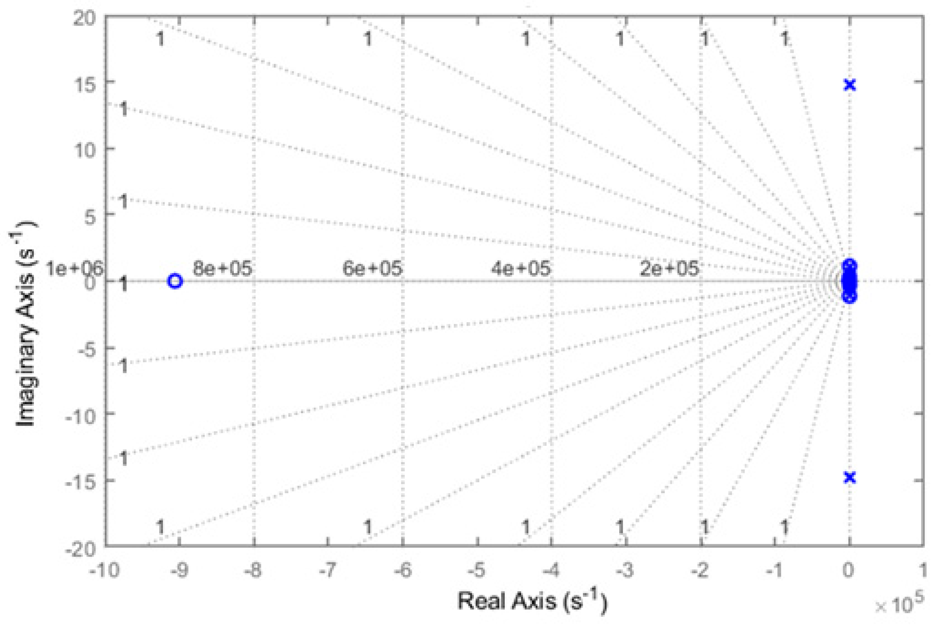
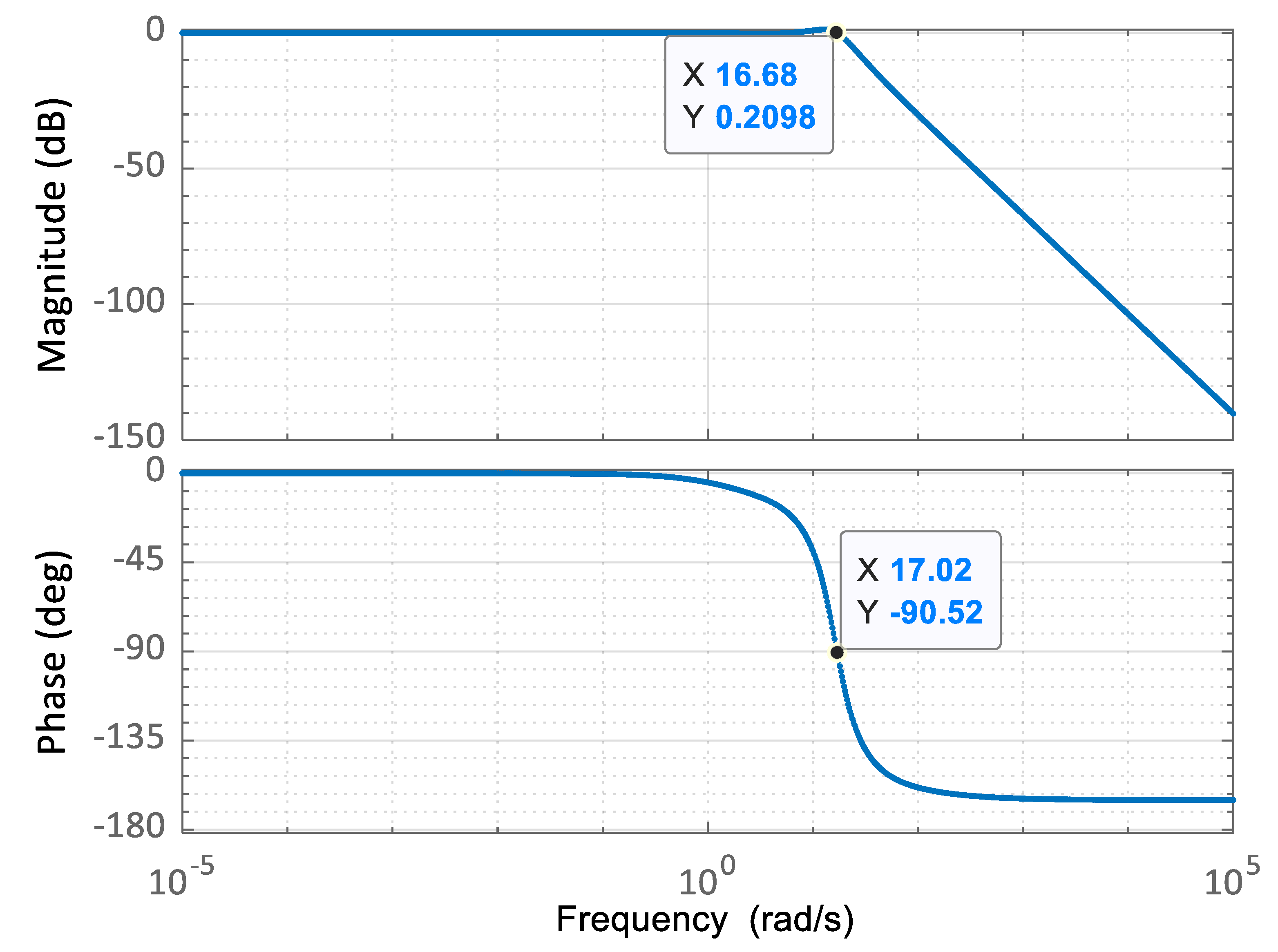
5.3. Stability Analysis

Figure 9 and Figure 10 show the pole/zero map and bode plot of the AVR system. The analysis of the bode plot and pole zeros was carried out in order to assess the stability of the system. The AVR system was derived using the controller parameters optimized by SSA. Therefore, the foremost analysis of the control system requires the assessment of the pole/zero map and bode plot.

Figure 9 shows that all the poles for the closed-loop AVR control system were found in the left half-plane of the s-graph. This is evidence of the stability and frequency response of the AVR system. Furthermore, since the phase never crosses −180° for all values of the gain, the gain margin for the system is said to be infinity which means the system is stable for all values of gain.

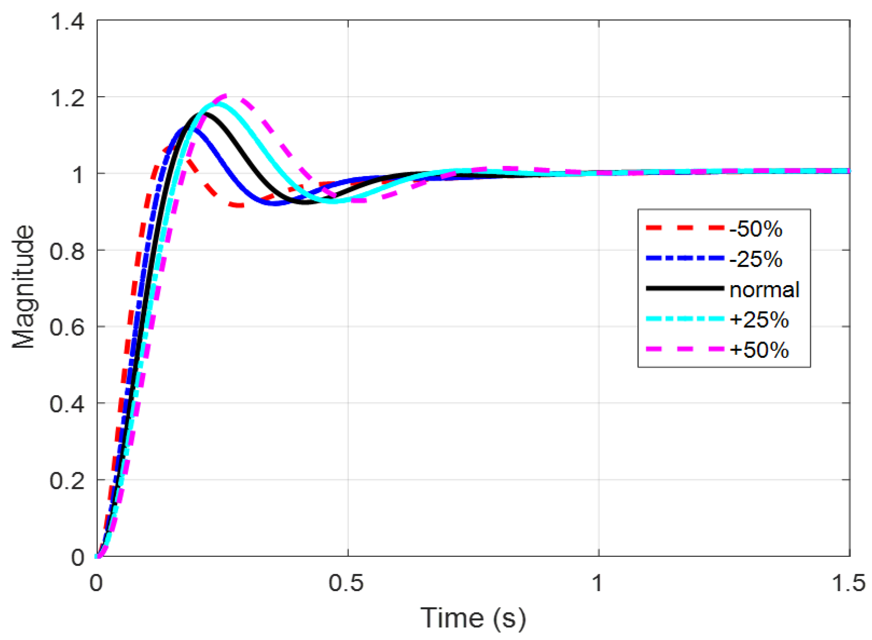
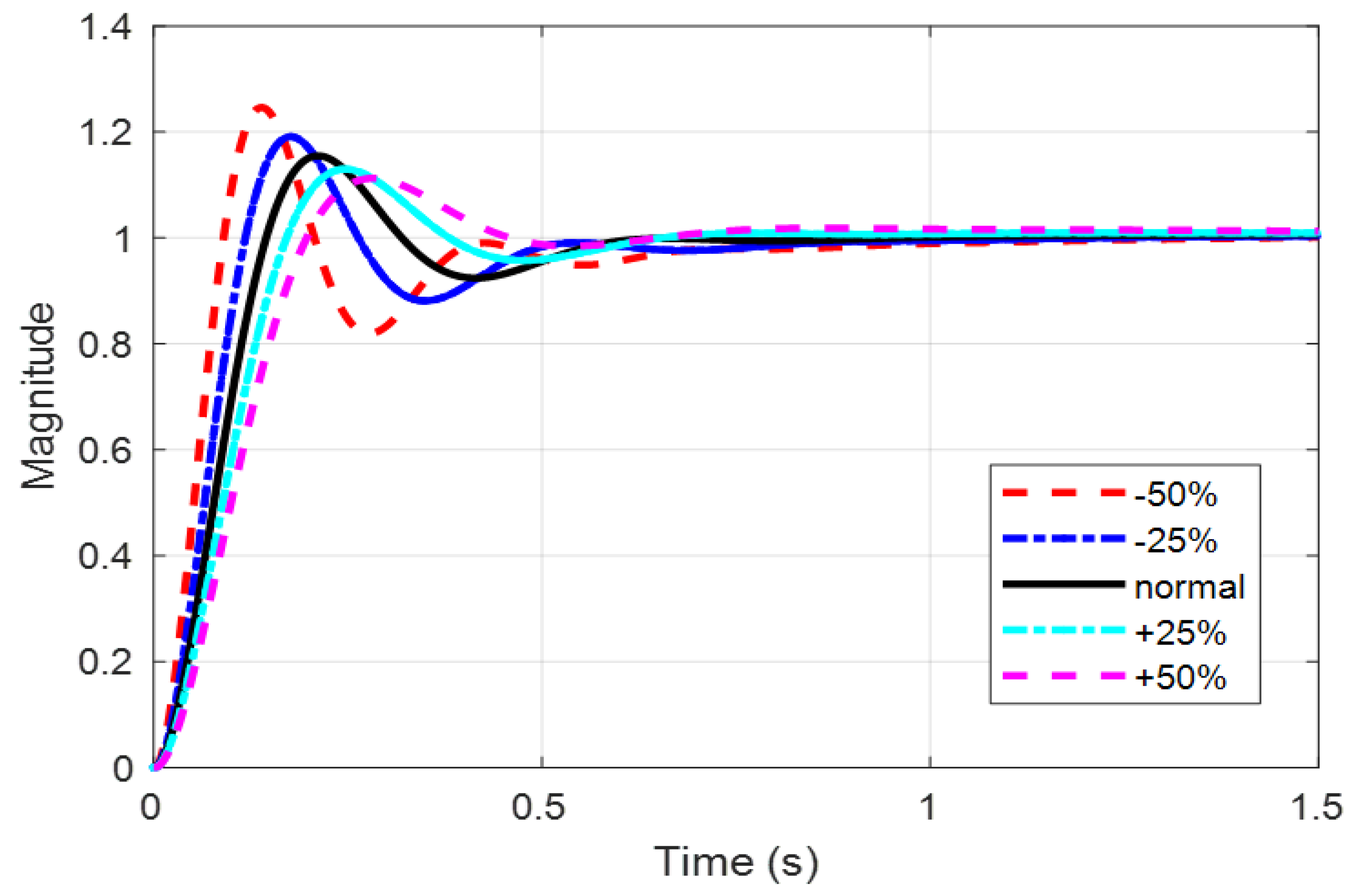
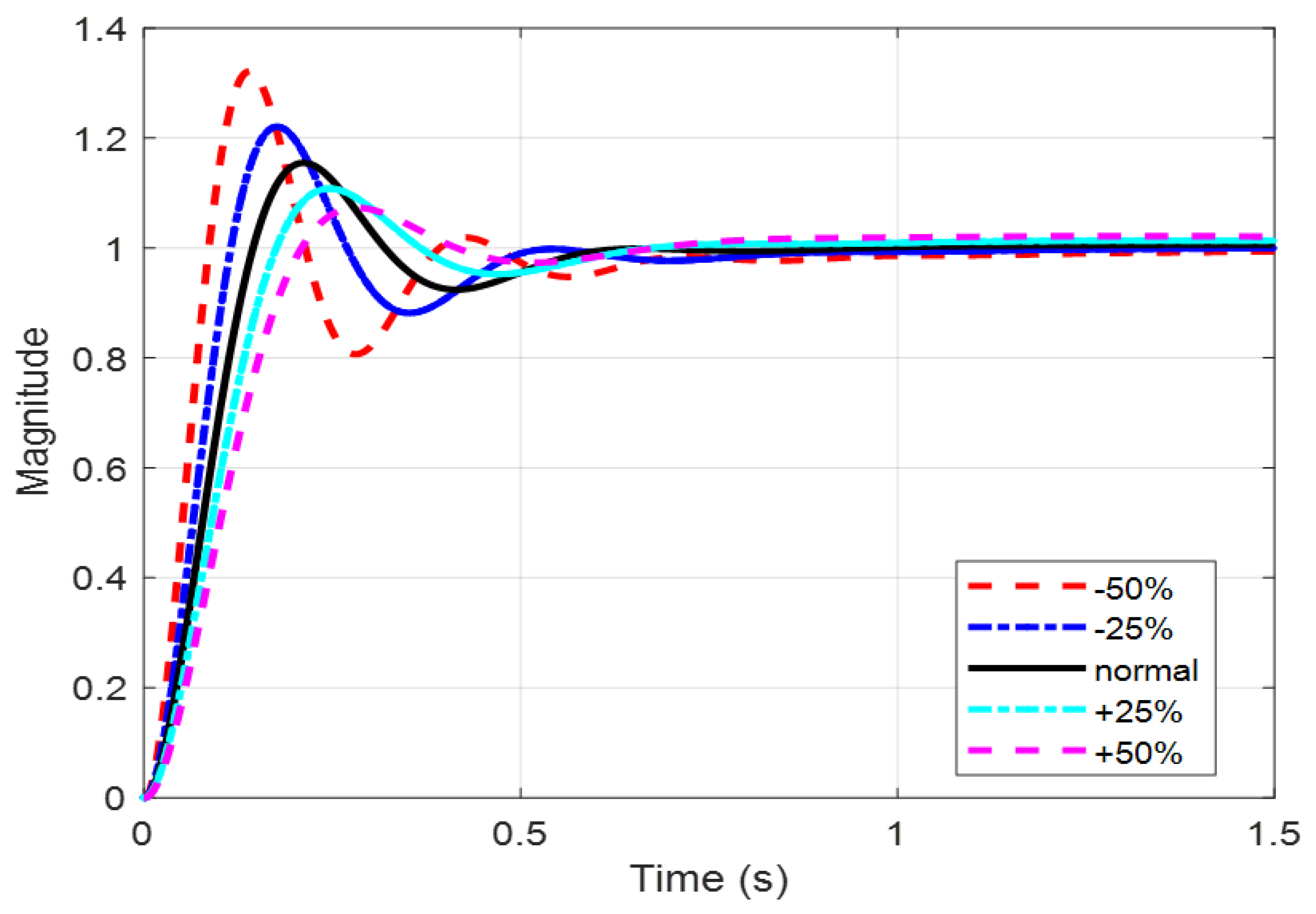
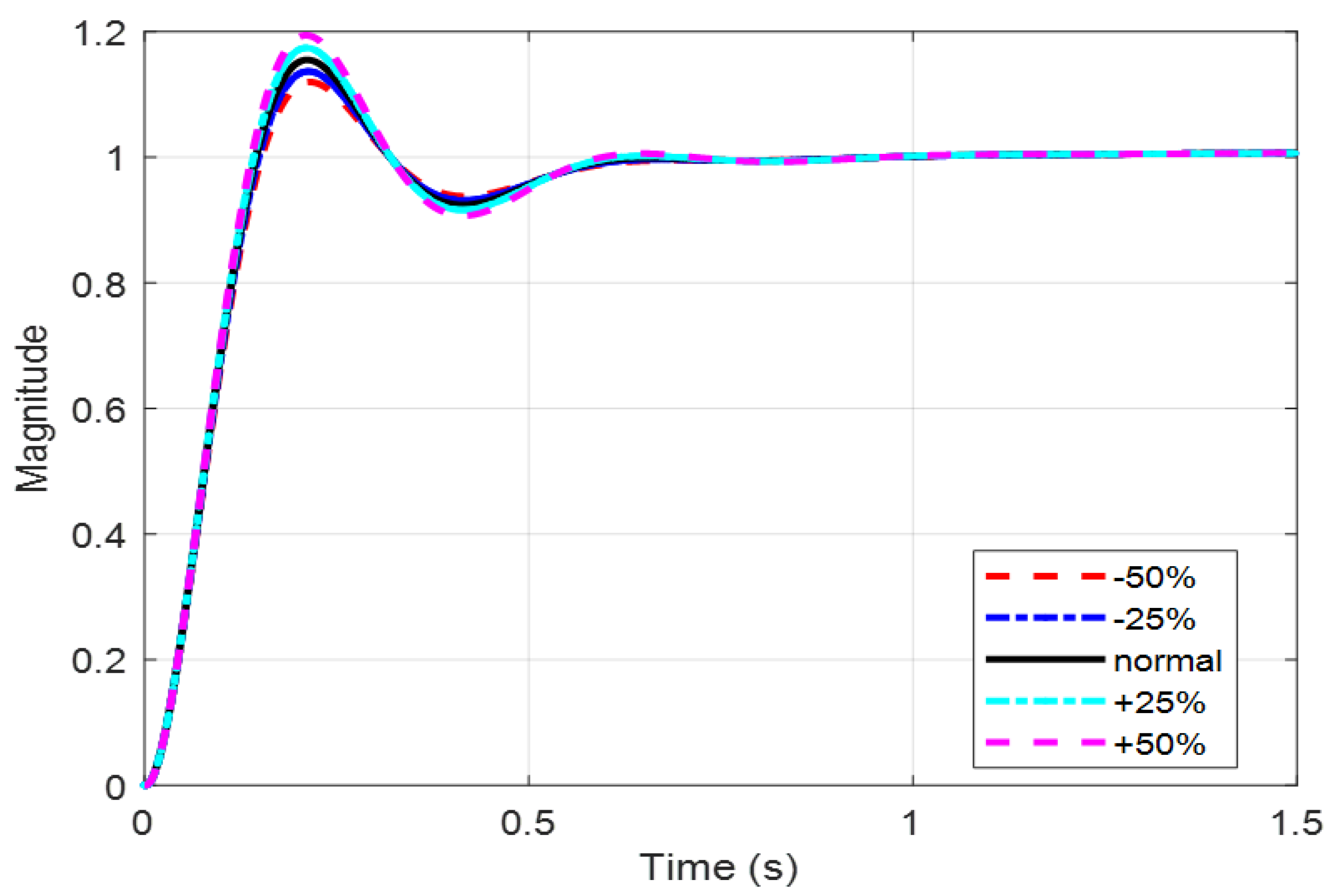
5.4. Robustness Analysis

Uncertainties in the control system parameters are a major cause of the instability. Therefore, a robustness analysis was carried out to assess the performance of the control system’s ability to surpass parameter uncertainty. This section focuses on the testing of the SSA-based AVR control system for uncertainties in the amplifier, exciter, generator, and sensor. The range of the variation was set to ±50% of the nominal values with a 25% step size. Corresponding responses are shown in Figure 11, Figure 12, Figure 13 and Figure 14.

It is observable from Figure 11, Figure 12, Figure 13 and Figure 14 that the system response curves only deviate within a small margin for a given time constant. This is major evidence of the ability of the proposed AVR controller in maintaining stability regardless of the variations in the parameters.

6. Conclusions

In this study, one of the most intelligent AI techniques called SSA was proposed in the design of an AVR system for the first time in the literature. The SSA is a self-adaptive algorithm with advanced convergence capabilities and showed better performance indicators than that of the other techniques used in recent state-of-the-art studies. The intelligence of the SSA was exploited to obtain the best combination of FOPID gains by minimizing a time integrating error fitness function. In order to assess the effectiveness of the proposed design, comparisons of the performance metrics were carried out with different optimization algorithms including DE [14], PSO [15], ABC [14], GOA [16], BBO [17], and PSA [18] on the basis of transient response and stability. The results showed that the FOPID controller tuned by SSA expresses improvement in transient response in comparison to alternate techniques in terms of Mp%, ts, tr, and tp values. Furthermore, from these analyses it was found that the system structure had good stability and the proposed SSA-FOPID controller was not affected by the changes in system parameters and, hence, proved to be robust against system parameter variations.

References

1. Ang, K.H.; Chong, G.; Li, Y. PID control system analysis, design, and technology. IEEE Trans. Control Syst. Technol. 2005, 13, 559–576. [Google Scholar]
2. Karimi-Ghartemani, M.; Zamani, M.; Sadati, N.; Parniani, M. An optimal fractional order controller for an AVR system using particle swarm optimization algorithm. In Proceedings of the 2007 Large Engineering Systems Conference on Power Engineering, Montreal, QC, Canada, 10–12 October 2007; pp. 244–249. [Google Scholar]
3. Tepljakov, A.; Alagoz, B.B.; Yeroglu, C.; Gonzalez, E.; HosseinNia, S.H.; Petlenkov, E. FOPID controllers and their industrial applications: A survey of recent results. IFAC PapersOnLine 2018, 51, 25–30. [Google Scholar] [CrossRef]
4. Podlubny, I. Fractional-order systems and PI/sup/spl lambda//D/sup/spl mu//-controllers. IEEE Trans. Autom. Control 1999, 44, 208–214. [Google Scholar] [CrossRef]
5. Li, X.; Wang, Y.; Li, N.; Han, M.; Tang, Y.; Liu, F. Optimal fractional order PID controller design for automatic voltage regulator system based on reference model using particle swarm optimization. Int. J. Mach. Learn. Cybern. 2017, 8, 1595–1605. [Google Scholar] [CrossRef]
6. Zamani, M.; Karimi-Ghartemani, M.; Sadati, N.; Parniani, M. Design of a fractional order PID controller for an AVR using particle swarm optimization. Control Eng. Pract. 2009, 17, 1380–1387. [Google Scholar] [CrossRef]
7. Ramezanian, H.; Balochian, S.; Zare, A. Design of optimal fractional-order PID controllers using particle swarm optimization algorithm for automatic voltage regulator (AVR) system. J. Control Autom. Electr. Syst. 2013, 24, 601–611. [Google Scholar] [CrossRef]
8. Lahcene, R.; Abdeldjalil, S.; Aissa, K. Optimal tuning of fractional order PID controller for AVR system using simulated annealing optimization algorithm. In Proceedings of the 2017 5th International Conference on Electrical Engineering-Boumerdes, Boumerdes, Algeria, 29–31 October 2017; pp. 1–6. [Google Scholar]
9. Aguila-Camacho, N.; Duarte-Mermoud, M.A. Fractional adaptive control for an automatic voltage regulator. ISA Trans. 2013, 52, 807–815. [Google Scholar] [CrossRef]
10. Pan, I.; Das, S. Chaotic multi-objective optimization based design of fractional order PIλDμ controller in AVR system. Int. J. Electr. Power Energy Syst. 2012, 43, 393–407. [Google Scholar] [CrossRef] [Green Version]
11. Jumani, T.A.; Mustafa, M.W.; Rasid, M.M.; Mirjat, N.H.; Baloch, M.H.; Salisu, S. Optimal Power Flow Controller for Grid-Connected Microgrids using Grasshopper Optimization Algorithm. Electronics 2019, 8, 111. [Google Scholar] [CrossRef] [Green Version]
12. Jumani, T.A.; Mustafa, M.W.; Rasid, M.M.; Mirjat, N.H.; Leghari, Z.H.; Saeed, M.S. Optimal Voltage and Frequency Control of an Islanded Microgrid using Grasshopper Optimization Algorithm. Energies 2018, 11, 3191. [Google Scholar] [CrossRef] [Green Version]
13. Li, M.; Du, W.; Nian, F. An adaptive particle swarm optimization algorithm based on directed weighted complex network. Math. Probl. Eng. 2014, 2014, 7. [Google Scholar] [CrossRef] [Green Version]
14. Gozde, H.; Taplamacioglu, M.C. Comparative performance analysis of artificial bee colony algorithm for automatic voltage regulator (AVR) system. J. Frankl. Inst. 2011, 348, 1927–1946. [Google Scholar] [CrossRef]
15. Sahib, M.A. A novel optimal PID plus second order derivative controller for AVR system. Eng. Sci. Technol. Int. J. 2015, 18, 194–206. [Google Scholar] [CrossRef] [Green Version]
16. Hekimoğlu, B.; Ekinci, S. Grasshopper optimization algorithm for automatic voltage regulator system. In Proceedings of the 2018 5th International Conference on Electrical and Electronic Engineering (ICEEE), Istanbul, Turkey, 3–5 May 2018; pp. 152–156. [Google Scholar]
17. Güvenç, U.; Işik, A.H.; Yiğit, T.; Akkaya, I. Performance analysis of biogeography-based optimization for automatic voltage regulator system. Turk. J. Electr. Eng. Comput. Sci. 2016, 24, 1150–1162. [Google Scholar] [CrossRef]
18. Sahu, B.K.; Panda, S.; Mohanty, P.K.; Mishra, N. Robust analysis and design of PID controlled AVR system using Pattern Search algorithm. In Proceedings of the 2012 IEEE International Conference on Power Electronics, Drives and Energy Systems (PEDES), Bengaluru, India, 16–19 December 2012; pp. 1–6. [Google Scholar]
19. Mukherjee, V.; Ghoshal, S. Intelligent particle swarm optimized fuzzy PID controller for AVR system. Electr. Power Syst. Res. 2007, 77, 1689–1698. [Google Scholar] [CrossRef]
20. Hosseinzadeh, M.; Salmasi, F.R. Robust optimal power management system for a hybrid AC/DC micro-grid. IEEE Trans. Sustain. Energy 2015, 6, 675–687. [Google Scholar] [CrossRef]
21. Schonberger, J.; Duke, R.; Round, S.D. DC-bus signaling: A distributed control strategy for a hybrid renewable nanogrid. IEEE Trans. Ind. Electron. 2006, 53, 1453–1460. [Google Scholar] [CrossRef]
22. Mirjalili, S.; Gandomi, A.H.; Mirjalili, S.Z.; Saremi, S.; Faris, H.; Mirjalili, S.M. Salp Swarm Algorithm: A bio-inspired optimizer for engineering design problems. Adv. Eng. Softw. 2017, 114, 163–191. [Google Scholar] [CrossRef]
23. Abbassi, R.; Abbassi, A.; Heidari, A.A.; Mirjalili, S. An efficient salp swarm-inspired algorithm for parameters identification of photovoltaic cell models. Energy Convers. Manag. 2019, 179, 362–372. [Google Scholar] [CrossRef]
24. Tolba, M.; Rezk, H.; Diab, A.; Al-Dhaifallah, M. A novel robust methodology based Salp swarm algorithm for allocation and capacity of renewable distributed generators on distribution grids. Energies 2018, 11, 2556. [Google Scholar] [CrossRef] [Green Version]
25. El-Fergany, A.A. Extracting optimal parameters of PEM fuel cells using Salp Swarm Optimizer. Renew. Energy 2018, 119, 641–648. [Google Scholar] [CrossRef]
26. Abusnaina, A.A.; Ahmad, S.; Jarrar, R.; Mafarja, M. Training neural networks using salp swarm algorithm for pattern classification. In Proceedings of the 2nd International Conference on Future Networks and Distributed Systems, Amman, Jordan, 26–27 June 2018; p. 17. [Google Scholar]
27. Kumari, S.; Shankar, G. A Novel Application of Salp Swarm Algorithm in Load Frequency Control of Multi-Area Power System. In Proceedings of the 2018 IEEE International Conference on Power Electronics, Drives and Energy Systems (PEDES), Madras, India, 18–21 December 2018; pp. 1–5. [Google Scholar]
28. Seborg, D.E.; Mellichamp, D.A.; Edgar, T.F.; Doyle, F.J., III. Process Dynamics and Control, 2nd ed.; John Wiley & Sons: Hoboken, NJ, USA, 2004. [Google Scholar]
29. Killingsworth, N.; Krstic, M. Auto-tuning of PID controllers via extremum seeking. In Proceedings of the American Control Conference 2005, Portland, OR, USA, 8–10 June 2005; pp. 2251–2256. [Google Scholar]
30. Jumani, T.A.; Mustafa, M.; Rasid, M.M.; Anjum, W.; Ayub, S. Salp Swarm Optimization Algorithm-Based Controller for Dynamic Response and Power Quality Enhancement of an Islanded Microgrid. Processes 2019, 7, 840. [Google Scholar] [CrossRef] [Green Version]
Figure 1. A typical arrangement of a simple automatic voltage regulator (AVR).
Electronics 08 01472 g001
Figure 2. The fractional-order proportional-integral-derivative (FOPID)-based AVR system.
Electronics 08 01472 g002
Figure 3. Proposed salp swarm optimization algorithm (SSA)-based FOPID parameter selection in the AVR system.
Electronics 08 01472 g003
Figure 4. Proposed FOPID tuning by SSA algorithm in the AVR system.
Electronics 08 01472 g004
Figure 5. Convergence curve for the proposed SSA for FOPID tuning in an AVR system.
Electronics 08 01472 g005
Figure 6. Comparison of the convergence behavior of the proposed algorithms with PSO, ABC, and GOA for the FOPID-based AVR system.
Electronics 08 01472 g006
Figure 7. AVR system step response with the SSA-optimized FOPID gains.
Electronics 08 01472 g007
Figure 8. Comparison of the proposed AVR FOPID tuning method with other methods used recently in the literature.
Electronics 08 01472 g008
Figure 9. Pole-zero map of the SSA-based AVR system.
Electronics 08 01472 g009
Figure 10. Bode analysis of the SSA-based AVR system.
Electronics 08 01472 g010
Figure 11. Amplifier gain change from −50% to 50%.
Electronics 08 01472 g011
Figure 12. Exciter gain change from −50% to 50%.
Electronics 08 01472 g012
Figure 13. Generator gain change from −50% to 50%.
Electronics 08 01472 g013
Figure 14. Sensor gain change from −50% to 50%.
Electronics 08 01472 g014