Performance Evaluation of Group Sparse Reconstruction and Total Variation Minimization for Target Imaging in Stratified Subsurface Media


Abstract
1. Introduction
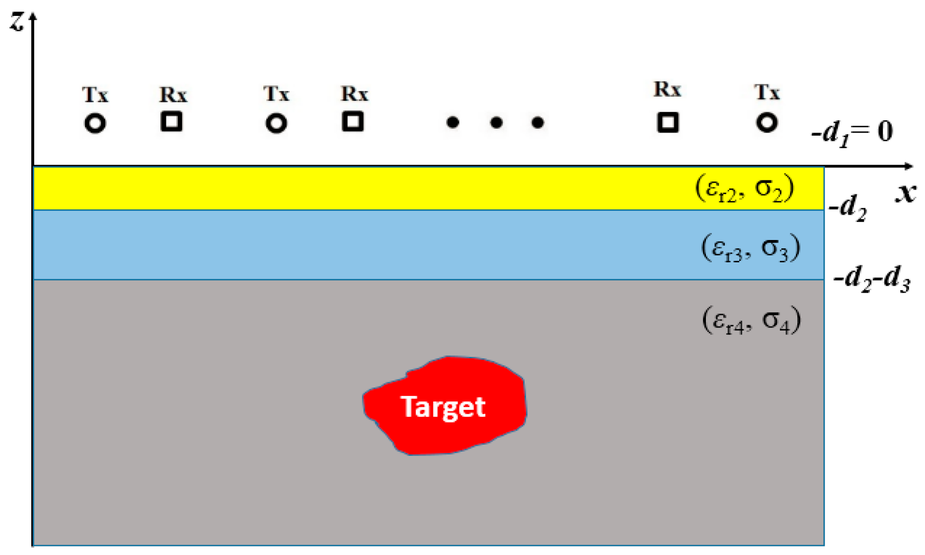
2. Sparsity-Based Image Formation through Stratified Subsurface Media
2.1. Signal Model in Matrix Form
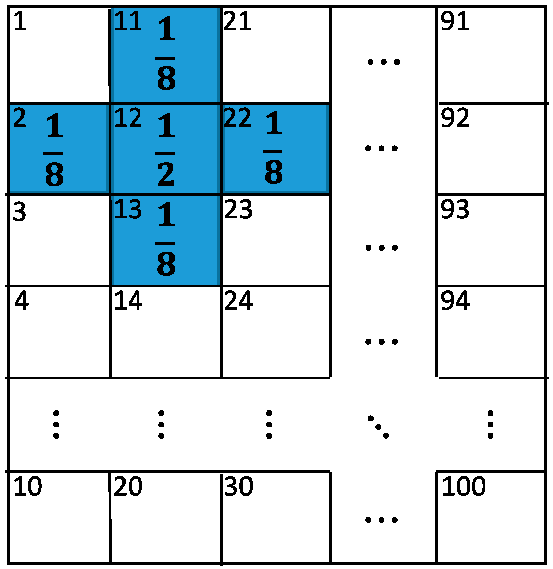
2.2. Total Variation Minimization
2.3. Group Sparse Reconstruction
3. Performance Evaluation Results and Discussion
3.1. Quantitative Metrics
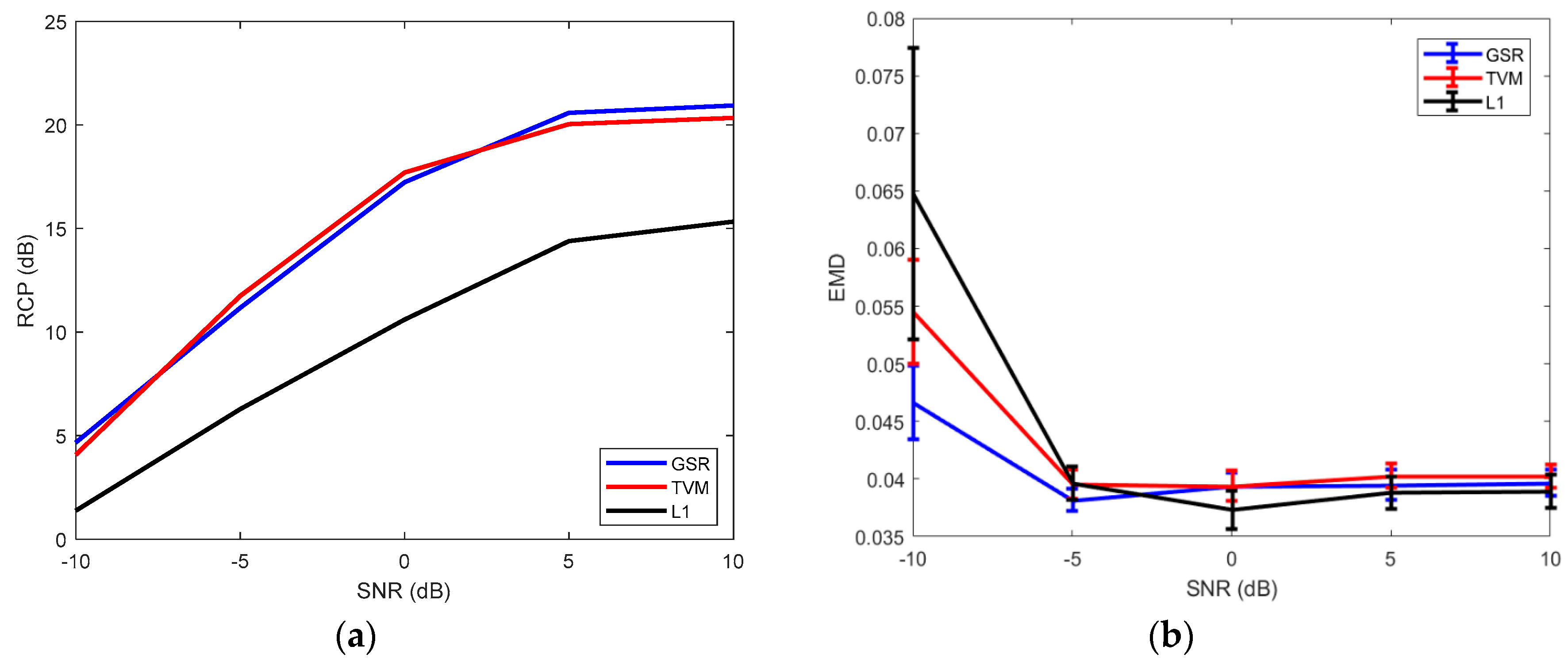
3.1.1. Relative Clutter Peak
3.1.2. Earth Mover’s Distance
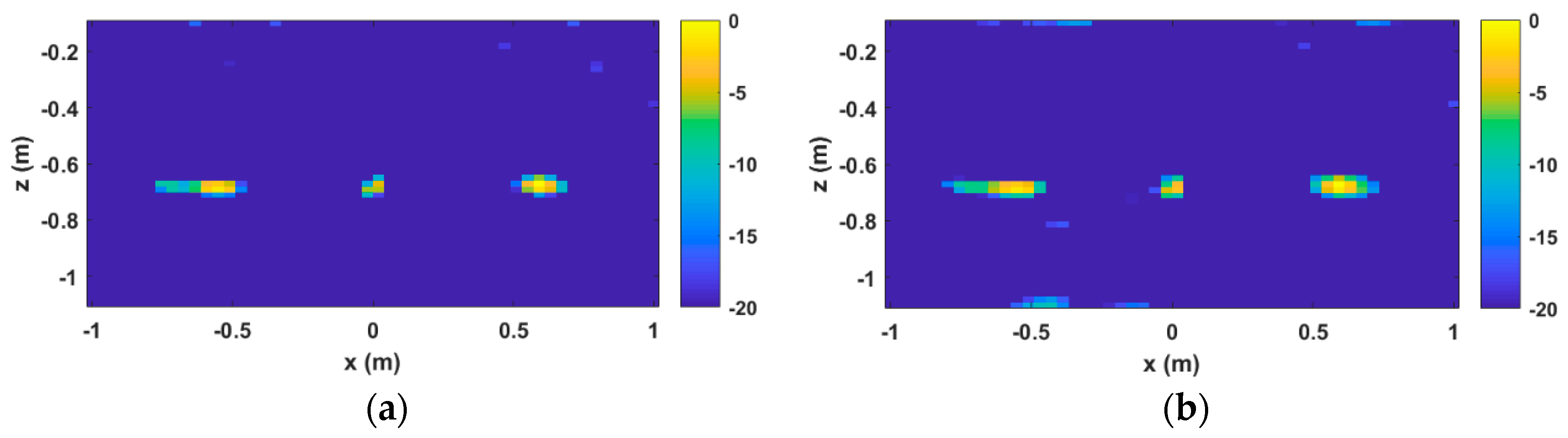
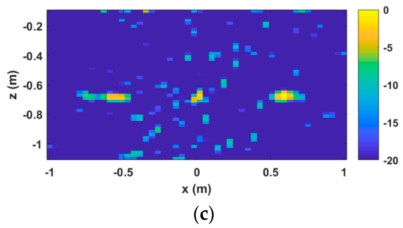
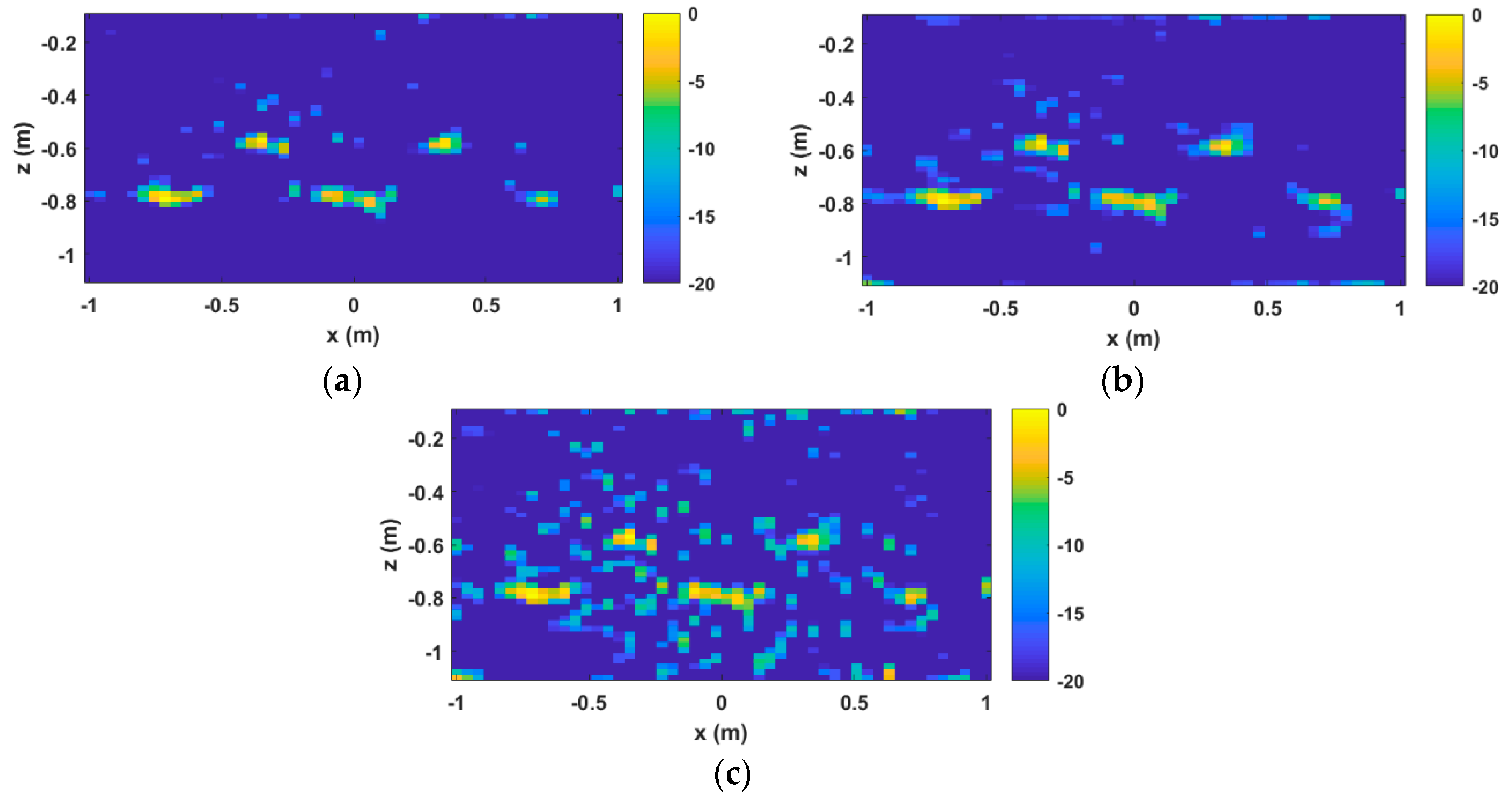
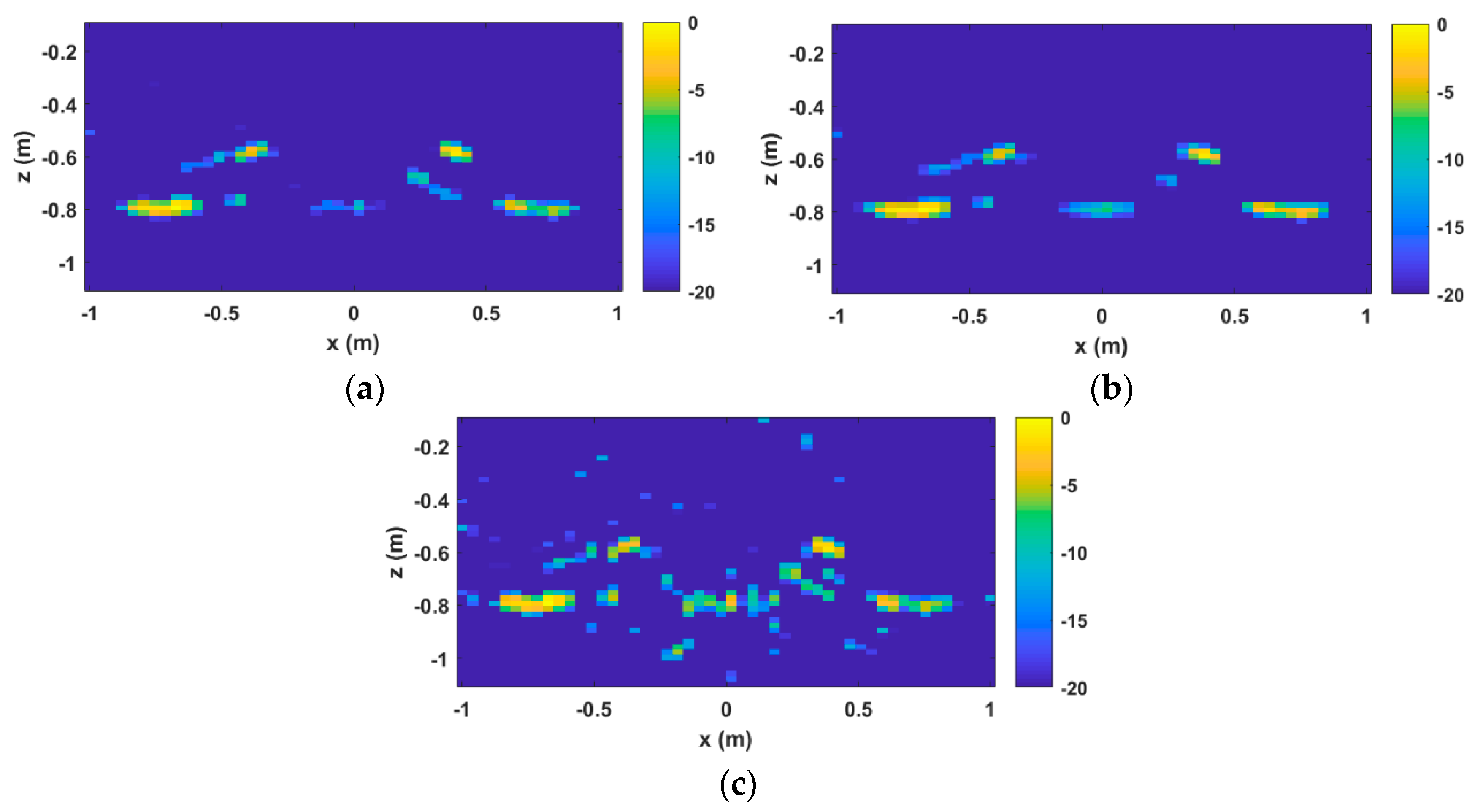
3.2. Performance Comparison
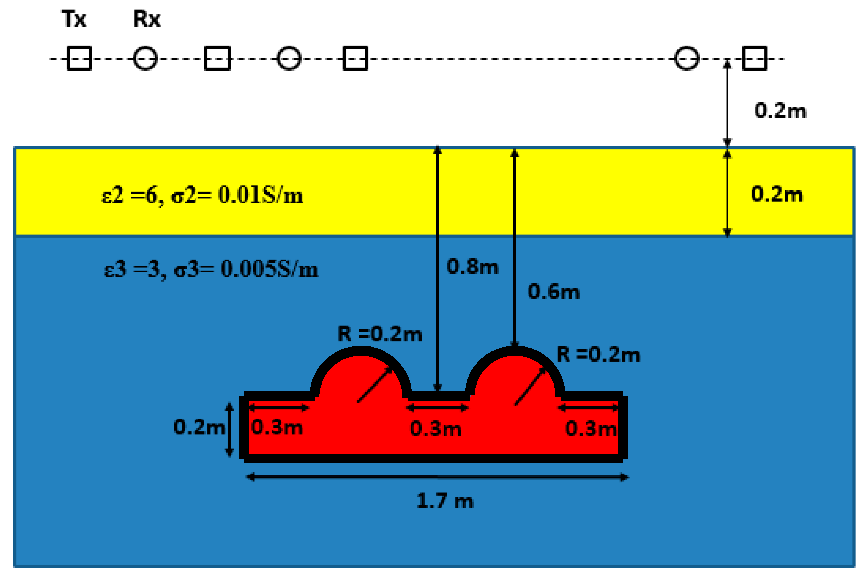
3.2.1. Example 1
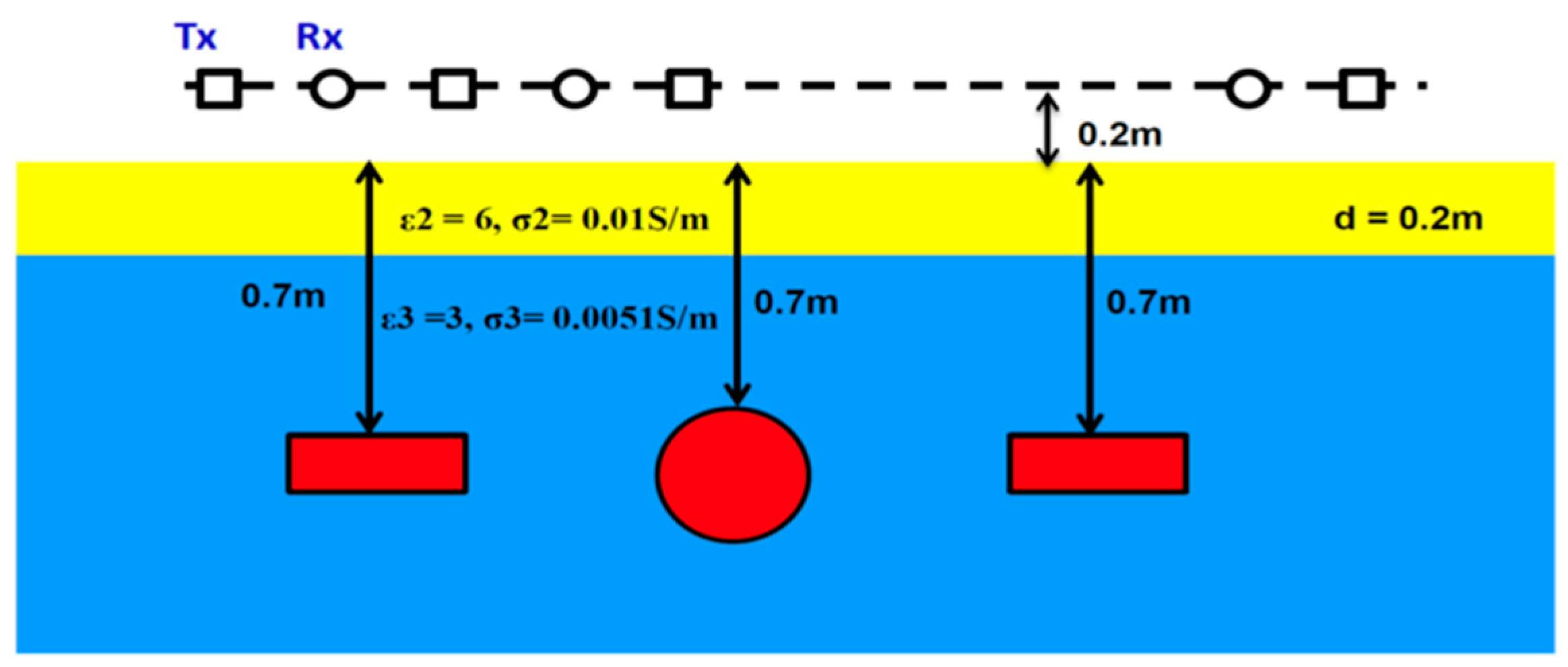
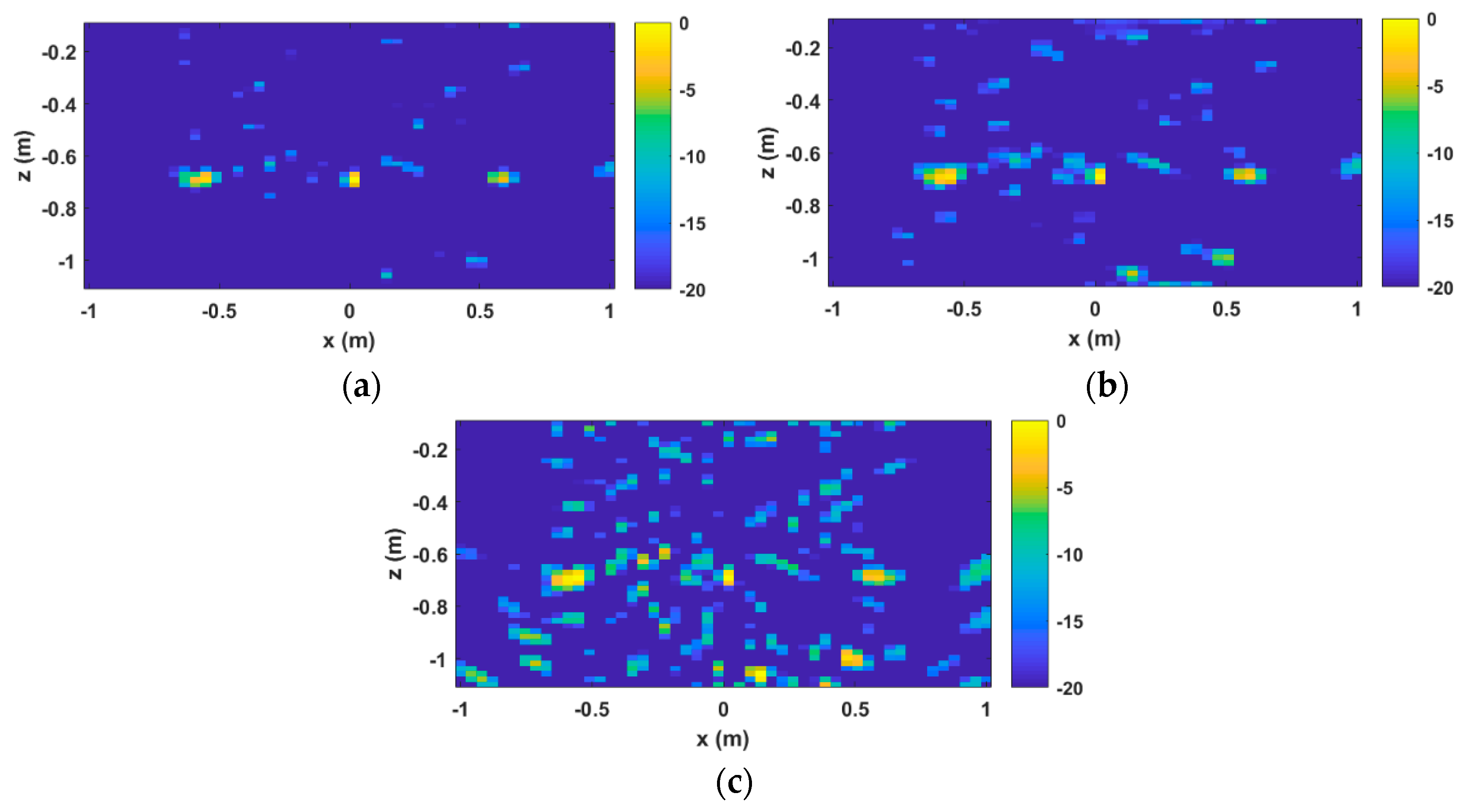
3.2.2. Example 2
3.3. Discussion
4. Conclusions
Author Contributions
Funding
Conflicts of Interest
References
- Persico, R. Introduction to Ground Penetrating Radar: Inverse Scattering and Data Processing; Wiley-IEEE Press: Hoboken, NJ, USA, 2014; ISBN 978-1-118-30500-3. [Google Scholar]
- Daniels, D.J. (Ed.) Ground Penetrating Radar, 2nd ed.; The Institution of Electrical Engineers: London, UK, 2004; ISBN 978-0-86341-360-5. [Google Scholar]
- Perisco, R.; Teixeira, F.L. Special Issue on Recent Progress in Ground Penetrating Radar Remote Sensing. Remote Sens. 2019, 11, 1864. [Google Scholar]
- Zhang, W.; Hoorfar, A. MIMO ground penetrating radar imaging through multilayered subsurface using total variation minimization. IEEE Trans. Geosci. Remote Sens. 2019, 57, 2107–2115. [Google Scholar] [CrossRef]
- Pambudi, A.D.; Fauss, M.; Ahmad, F.; Zoubir, A.M. Robust detection for forward-looking GPR in rough-surface clutter environments. In Proceedings of the 52nd Asilomar Conference on Signals, Systems, and Computers, Pacific Grove, CA, USA, 28–31 October 2018; pp. 2077–2080. [Google Scholar] [CrossRef]
- De Coster, A.; Lambot, S. Full-wave removal of internal antenna effects and antenna–medium interactions for improved ground-penetrating radar imaging. IEEE Trans. Geosci. Remote Sens. 2019, 57, 93–103. [Google Scholar] [CrossRef]
- Comite, D.; Ahmad, F.; Dogaru, T.; Amin, M.G. Adaptive detection of low-signature targets in forward-looking GPR imagery. IEEE Geosci. Remote Sens. Lett. 2018, 15, 1520–1524. [Google Scholar] [CrossRef]
- Camilo, J.A.; Collins, L.M.; Malof, J.M. A large comparison of feature-based approaches for buried target classification in forward-looking ground-penetrating radar. IEEE Trans. Geosci. Remote Sens. 2018, 56, 547–558. [Google Scholar] [CrossRef]
- Comite, D.; Ahmad, F.; Liao, D.; Dogaru, T.; Amin, M.G. Multiview imaging for low-signature target detection in rough-surface clutter environment. IEEE Trans. Geosci. Remote Sens. 2017, 55, 5220–5229. [Google Scholar] [CrossRef]
- Catapano, I.; Affinito, A.; Del Moro, A.; Alli, G.; Soldovieri, F. Forward-looking ground-penetrating radar via a linear inverse scattering approach. IEEE Trans. Geosci. Remote Sens. 2015, 53, 5624–5633. [Google Scholar] [CrossRef]
- Catapano, I.; Randazzo, A.; Slob, E.; Solimene, R. GPR imaging via qualitative and quantitative approaches. In Civil Engineering Applications of Ground Penetrating Radar; Springer Transactions in Civil and Environmental Engineering; Benedetto, A., Pajewski, L., Eds.; Springer: Cham, Switzerland, 2015. [Google Scholar]
- Wang, T.; Keller, J.M.; Gader, P.D.; Sjahputera, O. Frequency sub-band processing and feature analysis of forward-looking ground penetrating radar signals for land-mine detection. IEEE Trans. Geosci. Remote Sens. 2007, 45, 718–729. [Google Scholar] [CrossRef]
- Wang, Y.; Sun, Y.; Li, J.; Stoica, P. Adaptive imaging for forward-looking ground penetrating radar. IEEE Trans. Aerosp. Electron. Syst. 2005, 41, 922–936. [Google Scholar] [CrossRef]
- Estatico, C.; Fedeli, A.; Pastorino, M.; Randazzo, A. Buried object detection by means of a Banach-space inversion procedure. Radio Sci. 2015, 50, 41–51. [Google Scholar] [CrossRef]
- Estatico, C.; Fedeli, A.; Pastorino, M.; Randazzo, A. A multi-frequency inexact-Newton method in Banach spaces for buried objects detection. IEEE Trans. Antennas Propag. 2015, 63, 4198–4204. [Google Scholar] [CrossRef]
- Estatico, C.; Fedeli, A.; Pastorino, M.; Randazzo. Microwave imaging by means of Lebesgue-space inversion: An overview. Electronics 2019, 8, 945. [Google Scholar] [CrossRef]
- Yang, J.; Jin, T.; Huang, X.; Thompson, J.; Zhou, Z. Sparse MIMO array forward-looking GPR imaging based on compressed sensing in clutter environment. IEEE Trans. Geosci. Remote Sens. 2014, 52, 4480–4494. [Google Scholar] [CrossRef]
- Qu, L.; Yang, T. Investigation of air/ground reflection and antenna beamwidth for compressive sensing SFCW GPR migration imaging. IEEE Trans. Geosci. Remote Sens. 2012, 50, 3143–3149. [Google Scholar] [CrossRef]
- Soldovieri, F.; Solimene, R.; Lo Monte, L.; Bavusi, M.; Loperte, A. Sparse reconstruction from GPR data with applications to rebar detection. IEEE Trans. Instrum. Meas. 2011, 60, 1070–1079. [Google Scholar] [CrossRef]
- Gurbuz, A.C.; McClellan, J.H.; Scott, W.R. A compressive sensing data acquisition and imaging method for stepped frequency GPRs. IEEE Trans. Signal Process. 2009, 57, 2640–2650. [Google Scholar] [CrossRef]
- Ahmad, F.; Zhang, W.; Hoorfar, A. Performance comparison of total variation minimization and group sparse reconstructions for extended target imaging in multilayered dielectric media. In Proceedings of the SPIE 10658, Compressive Sensing VII: From Diverse Modalities to Big Data Analytics, Orlando, FL, USA, 18–19 April 2018; p. 106580I. [Google Scholar] [CrossRef]
- Wakin, M.B. Compressing Sensing Fundamentals. In Compressive Sensing for Urban Radar; Amin, M.G., Ed.; CRC Press: Boca Raton, FL, USA, 2015; pp. 1–48. [Google Scholar]
- Leigsnering, M.; Ahmad, F.; Amin, M.; Zoubir, A. Multipath exploitation in through-the-wall radar imaging using sparse reconstruction. IEEE Trans. Aerosp. Electronic Syst. 2014, 50, 920–939. [Google Scholar] [CrossRef]
- Qian, J.; Ahmad, F.; Amin, M.G. Joint localization of stationary and moving targets behind walls using sparse scene recovery. J. Electron. Imag. 2013, 22, 1–11. [Google Scholar] [CrossRef]
- Becker, S.; Bobin, J.; Candès, E.J. NESTA: A fast and accurate first-order method for sparse recovery. SIAM J. Imag. Sci. 2011, 4, 1–39. [Google Scholar] [CrossRef]
- Yuan, M.; Lin, Y. Model selection and estimation in regression with grouped variables. J. R. Stat. Soc. Ser. B 2006, 68, 49–67. [Google Scholar] [CrossRef]
- Deng, W.; Yin, W.; Zhang, Y. Group Sparse Optimization by Alternating Direction Method; Technical Report TR11-06; Department of Computational and Applied Mathematics, Rice University: Houston, TX, USA, 2011. [Google Scholar]
- Rubner, Y.; Tomasi, C.; Guibas, L.J. The Earth Mover’s Distance as a metric for image retrieval. Int. J. Comput. Vis. 2000, 40, 99–121. [Google Scholar] [CrossRef]
- Gupta, R.; Indyk, P.; Price, E. Sparse recovery for Earth Mover Distance. In Proceedings of the 48th Annual Allerton Conf. Communication, Control, and Computing, Monticello, IL, USA, 29 September–1 October 2010; pp. 1742–1744. [Google Scholar]
- Krueger, K.; McClellan, J.H.; Scott, W.R., Jr. 3-D imaging for groung penetrating radar using compressive sensing with block-toeplitz structures. In Proceedings of the IEEE 7th Sensor Array and Multichannel Signal Process. Workshop, Hoboken, NJ, USA, 17–20 June 2012; pp. 229–232. [Google Scholar]
- Pele, O.; Werman, M. Fast and robust earth mover’s distances. In Proceedings of the IEEE 12th Int. Conf. Computer Vision, Kyoto, Japan, 29 September–2 October 2009; pp. 460–467. [Google Scholar]
- Thajudeen, C.; Hoorfar, A.; Zhang, W. Estimation of frequency-dependent parameters of unknown walls for enhanced through-the-wall imaging. In Proceedings of the IEEE International Symposium Antennas Propagation URSI Meeting, Spokane, WA, USA, 3–8 July 2011; pp. 3070–3073. [Google Scholar] [CrossRef]
- Zarifi, D.; Farahbakhsh, A.; Abdolali, A.; Soleimani, M. Reconstructing constitutive parameters of inhomogeneous planar layered chiral media based on the optimization approach. Prog. Electromagn. Res. M 2013, 29, 29–39. [Google Scholar] [CrossRef]
- Spagnolini, U. Permittivity measurements of multilayered media with monostatic pulse radar. IEEE Trans. Geosci. Remote Sens. 1997, 35, 454–463. [Google Scholar] [CrossRef]
- Thajudeen, C.; Hoorfar, A. A hybrid bistatic-monostatic radar technique for estimation of lossy wall parameters. IEEE Antenn. Wireless Propag. Lett. 2016, 16, 1249–1252. [Google Scholar] [CrossRef]
- NESTA: A Fast and Accurate First-order Method for Sparse Recovery. Available online: http://statweb.stanford.edu/~candes/nesta/ (accessed on 23 October 2019).


| Type | Dimensions | Center Position |
|---|---|---|
| Rectangular | 0.2 m 0.1 m | (−0.6 m, −0.75 m) |
| Cylindrical | Radius = 0.1 m | (0, −0.8 m) |
| Rectangular | 0.2 m 0.1 m | (0.6 m, −0.75 m) |
© 2019 by the authors. Licensee MDPI, Basel, Switzerland. This article is an open access article distributed under the terms and conditions of the Creative Commons Attribution (CC BY) license (http://creativecommons.org/licenses/by/4.0/).
Share and Cite
Ahmad, F.; Hoorfar, A.; Zhang, W. Performance Evaluation of Group Sparse Reconstruction and Total Variation Minimization for Target Imaging in Stratified Subsurface Media. Electronics 2019, 8, 1245. https://doi.org/10.3390/electronics8111245
Ahmad F, Hoorfar A, Zhang W. Performance Evaluation of Group Sparse Reconstruction and Total Variation Minimization for Target Imaging in Stratified Subsurface Media. Electronics. 2019; 8(11):1245. https://doi.org/10.3390/electronics8111245
Chicago/Turabian StyleAhmad, Fauzia, Ahmad Hoorfar, and Wenji Zhang. 2019. "Performance Evaluation of Group Sparse Reconstruction and Total Variation Minimization for Target Imaging in Stratified Subsurface Media" Electronics 8, no. 11: 1245. https://doi.org/10.3390/electronics8111245
APA StyleAhmad, F., Hoorfar, A., & Zhang, W. (2019). Performance Evaluation of Group Sparse Reconstruction and Total Variation Minimization for Target Imaging in Stratified Subsurface Media. Electronics, 8(11), 1245. https://doi.org/10.3390/electronics8111245