Deployment of a Software to Simulate Control Systems in the State-Space

Abstract

In this work, we present a simulation software that permits designing and testing several types of controllers based on both classical and modern control theory. It has been created using Easy JavaScript Simulations, since this software permits implementing interactive simulations of physical systems in a quick and intuitive way. This laboratory contains a SISO (Single-Input and Single-Output) and a MIMO (Multiple-Input and Multiple-Output) plant, which are hydraulic and nonlinear, thus the linear model (linearized equations) and the original model (nonlinerized equations) have been implemented. The user can choose any of these physical systems and they have the options to control them using either continuous-time or discrete-time controllers. All parameters of the plant are fully configurable by the user. After that, the controller can be designed and tested. This simulation software offers several configurations: (a) PID (Proportional, Integral and Derivative controller); (b) state feedback; (c) observer and state feedback; and (d) integral controller, observer and state feedback control. The evolution of the controlled system is visualized using an animation of the virtual plant and a graphical representation of the evolution of the most important variables. In this paper, the steps for the implementation of this simulation software are detailed.

1. Introduction

Laboratory exercises are a fundamental part of education curricula in scientific and technological fields, such as computer science, engineering, natural sciences and others [1]. Students get theoretical knowledge in the classroom. However, laboratories are necessary to gain practical knowledge and experience [2]. The work in a traditional laboratory presents some disadvantages such as time and place restrictions for both students and academic staff. Another one is that this laboratory involves high costs associated with equipment [3], since the cost of purchasing and maintaining the necessary equipment is usually high, and often several units of the equipment must be available [4].

Other educational resources can be employed as an alternative or supplement to real laboratories. For instance, remote laboratories [5,6,7] use real plants and physical devices which are operated at distance [8]. This type of laboratory overcomes some of the traditional laboratory disadvantages. For instance, it is not necessary to find space for students to access the equipment. In addition, remote laboratories are cheaper than traditional ones, since having several units is not a requirement [9]. However, it means that only one student can access a particular equipment at a time. Besides, the implementation of this option can be complex, especially with regard to the communication and sensory-control hardware and software required [10].

On the contrary, the virtual laboratories [11,12,13,14] provide a cost-efficient alternative and several students can use the same virtual equipment at the same time. In addition, the student can access anytime and anywhere. Other advantage of the virtual system is that it permits configuring the parameters of the plant, which is often not possible in real systems. This type of laboratories constitute a useful teaching and learning environment where the physical system is virtualized by means of a series of simulations [15], thus the plant is not real. They can be implemented as desktop programs (running on the user’s operating system) or web-based applications (running on the user’s web browser) [16]. Nowadays, simulations have evolved into interactive graphical user interfaces where students can manipulate the experiment parameters and explore their evolution. This allows students to study different systems and, with basic programming skills, change the mathematical model or construct a new one [17]. It is worth highlighting that this simulation platform has been implemented as a supplementary tool, not an alternative tool. Thanks to it, students can familiarize with the calculation and initial implementation of controllers, before going to the real laboratory (where only a reduced number of sessions will be necessary).

Many examples of virtual laboratories in the field of control education can be found in the literature [18,19,20]. Most of them are designed to put into practice classical control techniques, based on the use of the transfer function. Modern control techniques, based on the use of the state-space representation, can be advantageous in some cases. The modern control is applicable to multiple-input, multiple-output (MIMO) systems, which may be linear or nonlinear, time invariant or time variant, while the classical control is typically applicable to linear time invariant single-input, single-output (SISO) systems [21].

In this work, we present a simulation software, implemented to ease the understanding of modern control techniques by the students. The software Easy Java/JavaScript Simulations (EJsS) [22,23] has been used to create the simulation software. EJsS is a free authoring tool designed for science students, teachers and researchers, and it permits creating simulations in a quick and simple way [24].

In comparison to other tools, EJsS presents several advantages for the development of simulation applications. The main one is that this tool does not focus on the technical programming aspects, but in the simulation itself. As a matter of fact, EJsS separates the design of the platform into modular parts: the implementation of the model (variables and evolution) and the visualization of the simulated model (view). Another advantage is that it simplifies the creation of a graphical user interface for simulations; EJsS offers a complete set of interactive components easily configurable to build it, according to the user needs of interactivity and visualization [25,26]. As mentioned above, the aim of this work is to create a simulation software which the students can run in a web browser from their house, hence EJsS has been chosen since it permits building it without the need for having a high knowledge about HTML programming. The implement is easy to replicate so other studies could use these developments to implement new simulation software with other plants or control methods.

The present paper continues and expands the work developed by Payá et al. [27], in which a virtual laboratory to control two different plants using controllers based either on classical or modern control theory is presented. However, the plants included are linear and SISO systems, and only continuous-time control is allowed. For this reason, the simulation software developed in the present paper includes new plants and control modes, in such a way that students can address more challenging problems. More concisely, two hydraulic plants are included and several control modes are available, based either on classical or on modern theory. The main contributions of this platform with respect to the previous work are threefold. (a) Either continuous-time or discrete-time controllers can be designed and tested in all cases. (b) A plant with multiple inputs and outputs is included, so that students can put into practice their knowledge in MIMO controllers. (c) Both plants are originally nonlinear systems; once the controller is designed, the student has the possibility of visualizing the behavior of the initially nonlinear system after adding the controller. It can be seen in the work developed by Galan et al. [28], since a hydraulic plant has been implemented and the behavior of the linear and original model are visualized. However, this virtual plant has only a single input and a single output and the options implemented to control it are manual control, PI/P controller and an on–off controller. Therefore, the work presented in the present paper offers a wider range of techniques, including state-space methods, to control a hydraulic system, and additionally one of the plants is a MIMO system.

In broad lines, the student has to complete the next steps to fully control a plant through this platform. These steps are developed in subsequent sections. First, the student must obtain the mathematical model of the original nonlinear system. All parameters that define the plant are fully configurable. Second, they must linearize the model around a working point to obtain either the transfer function or the state-space representation, depending on the control technique to use. Third, the kind of controller must be chosen. The options that our platform offers are classic and modern control. Within the classic control, students can design a PID controller while, in the case of modern control, the dynamics of the system can be controlled using state feedback and the user can also add a state observer and/or an integral controller to track the reference input. Fourth, once the type of control has been chosen, its parameters must be calculated. Thus far, the student has to model and design the control system manually, which allows them to put in practice the concepts studied in the classroom. Fifth, they can introduce the values of the controller in the platform and check if the system behaves according to the specifications. To this purpose, a simulation of the behavior of the system is shown and the user can introduce different reference inputs. Since the plants included in the platform are nonlinear and controllers are often obtained from the linearized model, it is interesting to check if the controller works correctly when used to control the original nonlinear plant. This platform permits visualizing both the linearized and the nonlinear model response. The behavior of the controlled system is shown using a virtual plant and a graphical representation of some relevant variables.

The main objective of the paper is to show the implementation that has been carried out in detail, focusing on the most relevant parts, providing all the necessary information so that other researchers can implement virtual laboratories in control engineering, based on these concepts. Additionally, the interface of the platform is shown and the modes of use, from the students’ point of view is remarked.

The remainder of the paper is structured as follows. In Section 2, the tool Easy Javascript Simulations is briefly presented. The implementation of the equations of the first plant, which is a SISO system, is described in Section 3 and the implementation of the controllers is detailed in Section 4. After that, Section 5 and Section 6 show the modeling of the second plant (MIMO system) along with the controllers. Section 7 presents the graphical interface of the platform and the results of some simulations. Finally, the conclusion and future works are outlined in Section 8.

The user can access this simulation software entering [29]. In addition, some laboratory guides are included on this platform website.

The previous sections contain the most relevant parts of the codes to carry out the implementation, the variables that appear are defined in Appendix A for a better understanding.

2. Easy JavaScript Simulations

In this section, Easy JavaScript Simulations (EJsS), which is the tool used to implement the simulation software, is briefly presented. Easy Java Simulations (EJS) permits creating interactive simulations of a physical system, showing the evolution of one or several variables that describe its state. The mathematical relations that define this state can be introduced in the platform in a relatively straightforward way. Therefore, EJsS eases the process to implement a virtual laboratory [22].

From release 5.0, the simulation can be created using also JavaScript and HTML5. In this work, the platform is implemented by means of JavaScript, due to the advantages it presents in comparison with Java. For instance, JavaScript simulations are more accessible since they can be run directly in standard web browsers. Besides, there are some technological devices that do not support Java applets, so in these cases JavaScript Simulations are a good solution.

This tool is based on the model–control–view paradigm, thus the simulation is divided into three parts that are deeply interconnected. The first one (model) describes the phenomenon or physical system by means of a set of variables and relationships among these variables. The second part (control) defines the user’s actions to have an influence upon the simulation. Finally, the third part (action) shows a graphical representation of the different states that the system may present.

To implement new simulations, EJsS offers a sequence of work panels (specifically three) that permit designing the model and its graphical user interface. They are denominated: Description, Model and View or HtmlView, being the last two the most important ones.

The Model panel is dedicated to define the mathematical model of the system. First, the variables and parameters that describe them must be declared and initialized. Then, the equations which determine how their values change in time have to be introduced. Finally, it is necessary to establish the behavior of the variables when the user interacts and modifies one or more of their values. To these purposes, the Model panel has six subpanels available, which are denominated Variables, Initialization, Evolution, Fixed Relations, Custom and Elements.

The evolution subpanel provides two ways to implement the equations that describe the evolution in time: by means of direct mathematical expressions or first-order differential equations. On the one hand, the first alternative is carried out in a page of code, and it only requires instructions in JavaScript language. On the other hand, the second alternative can be performed by creating a page of EDOs (Ordinary Differential Equation). Apart from the equations, three parameters must be defined in this page, which affect how the simulation is computed and displayed. They are the increment, the number of Frames Per Second (FPS) and the number of Steps Per Display (SPD). The last one determines how many steps must advance the evolution of the model before refreshing the graphical representation. To solve these differential equations, a solver algorithm must be chosen.

The View/HtmlView panel permits building the graphical user interface by selecting elements from palettes and adding them to the view’s tree of elements. It determines the user interaction with the model and shows a schematic or realistic representation of the phenomenon or system. In the case of HtmlView, the interface elements present CSS properties.

3. Implementation of the First Plant (SISO System). Mathematical Model

The first system implemented in the simulation software is a SISO system (Single-Input and Single-Output). As commented above, the tool EJsS has been used. Section 3.1 describes succinctly this system. After that, the next subsections present the implementation of the system equations in EJsS. First, Section 3.2 details the steps for the linearized version, and then Section 3.3 for the original nonlinear model. Section 3.4 describes the implementation of the saturation block.

3.1. System Description

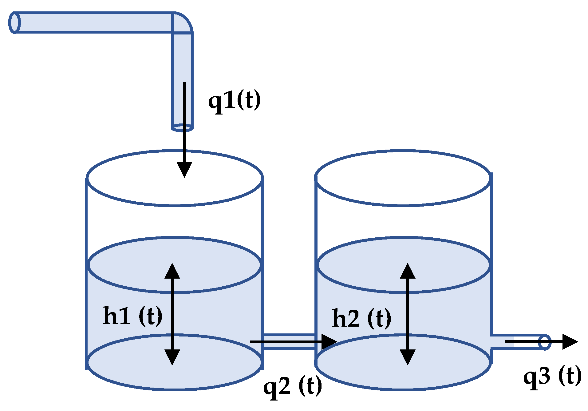
The plant is composed of two consecutive tanks, as shown in Figure 1. The first one is supplied by a flow $q1\left(t\right)$ which is the system input. The output variable is the height of the second tank $h2\left(t\right)$.

The parameters of the process are the cross section of each tank ($A1$ and $A2$) and the discharge coefficients ($r1$ and $r2$). The user can freely configure these parameters before starting any simulation.

Furthermore, the variables are the input flow $q1\left(t\right)$, the flow from the first to the second tank $q2\left(t\right)$, the output flow of the second tank $q3\left(t\right)$, the fluid level of the first tank $h1\left(t\right)$ and the fluid level of the second tank $h2\left(t\right)$. Once the parameters and variables are defined, the equations of this system are:

$$q2\left(t\right)=r1\sqrt{h1\left(t\right)-h2\left(t\right)}$$

(1)

$$q3\left(t\right)=r2\sqrt{h2\left(t\right)}$$

(2)

$$A1·\frac{dh1\left(t\right)}{dt}=q1\left(t\right)-q2\left(t\right)$$

(3)

$$A2·\frac{dh2\left(t\right)}{dt}=q2\left(t\right)-q3\left(t\right)$$

(4)

In this hydraulic system, one can consider the fluid heights of both tanks as the physical state variables. In addition, it is worth highlighting the fact that this plant is nonlinear. For this reason, if linear techniques are used to calculate the controller, the student must linearize it around a working point, obtaining either its transfer function or its state space representation. Both the linearized system and the original nonlinear model have been implemented in the same HTML page. The user can choose the type of equations to be used for the simulation (linearized or original model) at the parameters window. The plant can be controlled in either continuous- or discrete-time. For this reason, two different HTML pages have been created.

In brief, the user will open one or another page depending on the kind of controller (continuous- or discrete-time). Then, they will choose the set of equations (original nonlinear or linearized) to simulate. The codes to carry out the implementation of this system are shown in the next sections, with the purpose of easing the understanding of them and the replication or implementation of new laboratories. All the variables and parameters that appear are defined in Appendix A.1.

3.2. Implementation of the Linearized Model

To implement both models, the first step is to define the parameters and variables which characterize each mathematical model. That is to say, in the case of the original nonlinear system, it is necessary to define the variables of the plant and, in the case of the linearized system, the working point and the incremental variables around it must be defined.

Apart from the variables of the plant, there are some other variables, e.g. time, which has been initialized to zero for starting the simulation at that instant of time, and its differential, which is necessary to write the differential equations. As described in the next sections, the controllers included in the platform are obtained from the linearized system. Therefore, they work with incremental variables. For this reason, it is necessary to obtain the incremental value of the reference height (h2ref_inc), whose value is introduced by the user (h2ref). The code is shown in Listing 1. It has been implemented in the fixed relations panel, since it does not depend on the simulated model.

Listing 1. Fixed relations panel (SISO).

h2ref_inc=h2ref-h20;

Once all the variables are defined, the equations that describe the behavior of the system must be introduced in the evolution method panel. This subsection focuses on the implementation of the linearized model; thus, the defined equations to define are those obtained after linearizing the equations of Section 3.1 around a working point. The equations of the plant are continuous-time, consequently are included on an ODE page, as shown in

Table 1. Differential equations of linearized system (linear SISO).

State	Derivative
$\frac{dh1\_inc\left(t\right)}{dt}$	$height1\_L(h1\_inc,h2\_inc,q1\_inc)$
$\frac{dh2\_inc\left(t\right)}{dt}$	$height2\_L(h1\_inc,h2\_inc)$

. To solve the differential equations, the Runge–Kutta method has been selected [30].

As shown in Table 1, two functions have been created in the custom methods panel and they are invoked from the ODE page to compute the differential equations. These functions are included in Listings 2 and 3.

The first function, whose code is shown in Listing 2, receives the values of the incremental variables of the first tank height (h1_inc), second tank height (h2_inc) and the input flow (q1_inc). The first derivative of h1_inc is calculated using Equation (3), but, before that, the incremental flow between both tanks (q2_inc) must be obtained by means of Equation (1) after linearized.

The code implemented in each function must limit that the final height of the fluid cannot be negative, since it is physically impossible. Therefore, when it happens, the height is saturated to zero and the differential equation is solved considering it. In other words, a lower limit must be defined for both heights. In the case of the linearized model, the heights (h1_inc and h2_inc) will not be lower than their value at the operating point (h10 and h20), but with negative sign.

Listing 2. Function to obtain the height of the first tank h1: height1_L (linear SISO).

function height1_L (h1_inc,h2_inc,q1_inc) {

if(h1_inc<-h10){

h1_inc=-h10;

}

if(h2_inc<-h20){

h2_inc=-h20;

}

//flow between both tanks

q2_inc=((r1*h1_inc*(1/(2*Math.sqrt(h10-h20))))-(r1*h2_inc*(1/(2*Math.sqrt(h10-h20)))));

return((1/A1)*(q1_inc-q2_inc)); //compute first derivative of H1

}

The code implemented in the second function, as shown in Listing 3, computes the incremental variables of the flow between both tanks (q2_inc) and the output flow of the second tank (q3_inc), the last one by means of Equation (2) but linearized. Finally, Equation (4) is used to obtain the first derivative of the second tank height.

Listing 3. Function to obtain the height of the second tank h2: height2_L (linear SISO).

function height2_L (h1_inc,h2_inc){

if(h1_inc<-h10){

h1_inc=-h10;

}

if(h2_inc<-h20){

h2_inc=-h20;

}

//flow between both tanks

q2_inc=((r1*h1_inc*(1/(2*Math.sqrt(h10-h20))))-(r1*h2_inc*(1/(2*Math.sqrt(h10-h20)))));

// tank 2 output flow

q3_inc=r2*(1/(2*Math.sqrt(h20)))*h2_inc;

return((1/A2)*(q2_inc-q3_inc)); // compute first derivative of H2

}

To end the implementation of the linearized model, it is necessary to take it into account that the evolution of some variables must be shown to the user. However, the values obtained with these equations are incremental, so the working point must be added to these values. Consequently, a code page (Listing 4) has been created, on which these operations are carried out.

Listing 4. Code page: Linearized system (linear SISO).

h1=h1_inc+h10;

h2=h2_inc+h20;

q1=q1_inc+q10;

3.3. Implementation of the Original Nonlinear Model

The original nonlinear model is composed of the equations shown in Section 3.1. They are continuous-time differential equations; thus, an ODE page (

Table 2. Differential equations of original system (nonlinear SISO).

State	Derivative
$\frac{dh1\_inc\left(t\right)}{dt}$	$height1\_NL(h1,h2,q1)$
$\frac{dh2\_inc\left(t\right)}{dt}$	$height2\_NL(h1,h2)$

) has been created to solve them.

As in the case of the linearized model, two functions, whose codes are shown in Listings 5 and 6, have been created to define the equations of this model and the behavior of the fluid heights. Their values cannot be negative, so the lower value of these variables is set to zero, when the equations are solved. Besides, a difference between both heights appear in a square root, as shown as Equation (1). For this reason, the result of this difference must be checked too. If the fluid height of the first tank $h1\left(t\right)$ is lower than the fluid height of the second tank $h2\left(t\right)$, then the direction of the flow between both tanks $q2\left(t\right)$ is opposite. In other words, the fluid will flow from the second tank to the first one.

Listing 5. Function to obtain the height of the first tank h1: height1_NL (nonlinear SISO).

function height1_NL (h1, h2, q1) {

if (h1<0){

h1=0;

}

if(h2<0){

h2=0;

}

if (h1 < h2) {

q2=-r1*Math.sqrt(h2-h1);

else {

q2=r1*Math.sqrt(h1-h2);

}

h1_inc=h1-h10; ; // compute the incremental value of h1

return (1/A1)*(q1-q2);

}

Listing 6. Function to obtain the height of the second tank h2: height2_L (nonlinear SISO).

function height2_NL (h1, h2) {

if (h1<0){

h1=0;

}

if(h2<0){

h2=0;

}

if (h1 < h2) {

q2=-r1*Math.sqrt(h2-h1);

else {

q2=r1*Math.sqrt(h1-h2);

}

h2_inc=h2-h20; ; // compute the incremental value of h1

return (1/A2)*(q2-r2*Math.sqrt(h2));

}

An important aspect is that the controllers included in the platform are calculated from the linearized plant, hence the variables involved in the controller must be incremental.

To carry out the control, the feedback of some variables is necessary. In other words, these variables are inputs to the controller, thus the working point must be subtracted from their values to obtain the incremental variables. On the contrary, the operating point will be added to the output variables of the controller, that is to say, to the calculated control action. These operations are carried out on a code page.

3.4. Saturation

Sometimes, the control action takes values which are not admissible when a system is controlled, since their values are limited in the real system. For this reason, an optional saturation block has been implemented for the control action. The user can activate it and set the maximum and minimum values of these variables (control action). The code to perform this behavior is implemented in each of the code pages created for each of the control techniques.

As shown in Listing 7, some new variables have been defined in a variable page to describe the behavior of the saturation block. For example, two boolean variables (sat_upper and sat_low) that determine if the user has activated the upper and/or lower saturation by means of a checkbox.

Listing 7. Code page: Saturation block (SISO).

if(sat_upper){

if (q1_inc+q10 > value_sat_upper){

q1_inc=value_sat_upper-q10;

}

}

if(sat_low){

if(q1_inc+q10 < value_sat_low){

q1_inc=value_sat_low-q10;

}

}

4. Implementation of the First Plant (SISO System). Controllers

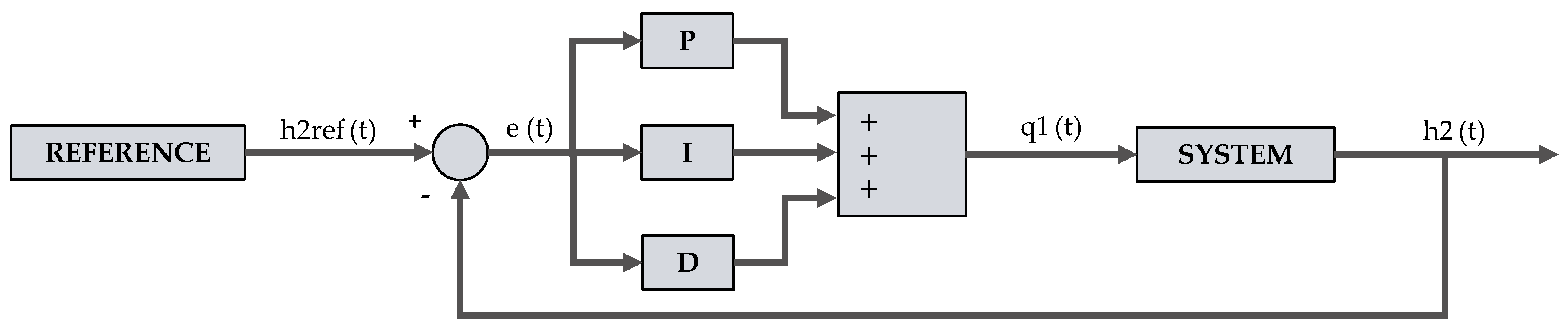
The purpose of this work consists in developing a simulation software that permits controlling some virtual systems, such as the plants described in the previous section. Several kinds of control techniques have been included in the platform, based on both classic and modern approaches. For example, Figure 2 shows the block diagram of a PID controller.

This section describes in detail the different kinds of controllers that the student can define, and how they are implemented in the platform. More information about the implementation of the controllers can be found in [21,31]. Section 4.1 focuses on the implementation of the controllers based on classical theory (continuous-/discrete-time) and Section 4.2 describes the implementation of the controllers based on modern theory (continuous-/discrete-time).

4.1. Classical Control Theory

This subsection presents the implementation of the PID controller. To describe the behavior of this kind of controller, first some parameters must be defined, such as the proportional ($kp$), derivative ($kd$) and integral ($kint$) constants, as well as the error signal ($error$), and its derivative ($derror$) and integral ($ei$). All these variables are included on the page of variables.

The platform permits controlling the system in either continuous- or discrete-time, so this subsection is divided into two parts.

4.1.1. Continuous-Time

The control action is obtained as a result of adding the integral, proportional and derivative actions that constitute the PID controller. The integral action must be expressed as a differential equation so that EJsS can calculate it. Therefore, to include it in the platform, we use the inverse operation, as shown in

Table 3. ODE page of classical control (SISO system).

State	Derivative
$\frac{dei}{dtime}$	error

. If the result of integrating the error is derived, the error is obtained. This equation is defined in the ODE page corresponding to this type of control and with the differential equations of the plant.

By contrast, the derivative and proportional parts have been implemented on a code page (Listing 8), as well as the final equation of the controller. The error signal is the difference between the incremental value of the reference and the incremental value of the output. In this platform, the first one is assumed to be a constant. Therefore, the derivative of the error is the value of the first derivative of the output (h2_d) with negative sign.

The equations of the control block do not depend on the model being used; however, it is important to calculate the derivative of the error (h2_d), thus its calculation is implemented in the function corresponding to the height of the second tank.

Listing 8. Code page: Continuous-time PID controller (SISO system).

error=h2ref_inc-h2_inc;

derror=-h2_d; // value computed in function height2

q1_inc=kp*error+kint*ei+kd*derror; //control action

4.1.2. Discrete-Time

The philosophy to implement the discrete controller changes substantially with respect to the method presented in the previous subsection for the continuous-time controller, because the system now contains both a continuous-time part (the plant) and a discrete-time part (the controller).

Therefore, the behavior of the discrete-time controller must be implemented on a code page, as shown in Listing 9, in such a way that only the differential equations of the plant are included in the ODE page.

The controller only makes calculations at specific moments of time (sampling instants). Thus, the code must check if the simulation time coincides with a sampling instant. In this case, the values of the variables will be kept until the next sampling instant (a zero-order hold is used to reconstruct the control action).

Listing 9. Code page: Discrete-time PID controller (SISO system).

if ((Math.round(time/dt))% (Ts/dt) === 0){

//Derivative

derror=(h2ref_inc-h2_inc)-error; //error[k]-error[k-1]

//Proportional

error=h2ref_inc-h2_inc;

//Integral

ei=error+ei; //error[k]+error[1:k-1]

q1_inc=kp*error+ki*ei+kd*derror;

}

else{

error=error;

derror=derror;

ei=ei;

q1_inc=q1_inc;

h2_inc=h2_inc;

}

In this case, the integral part is obtained using the product of the integral constant and the sum of the values of the error signal, since the beginning of the simulation until the actual sampling instant. Additionally, the derivative of the error signal is calculated as the difference between its current value and its value at the previous sampling instant.

4.2. Modern Control Theory

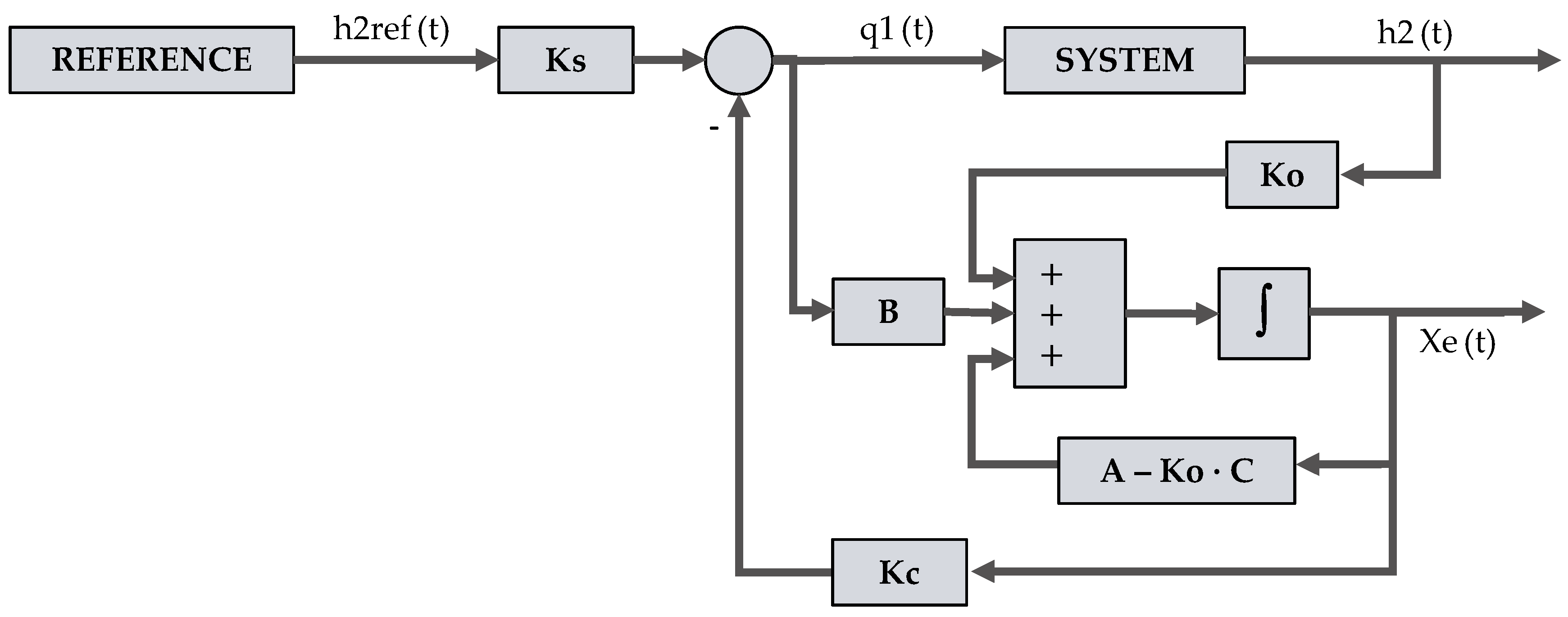
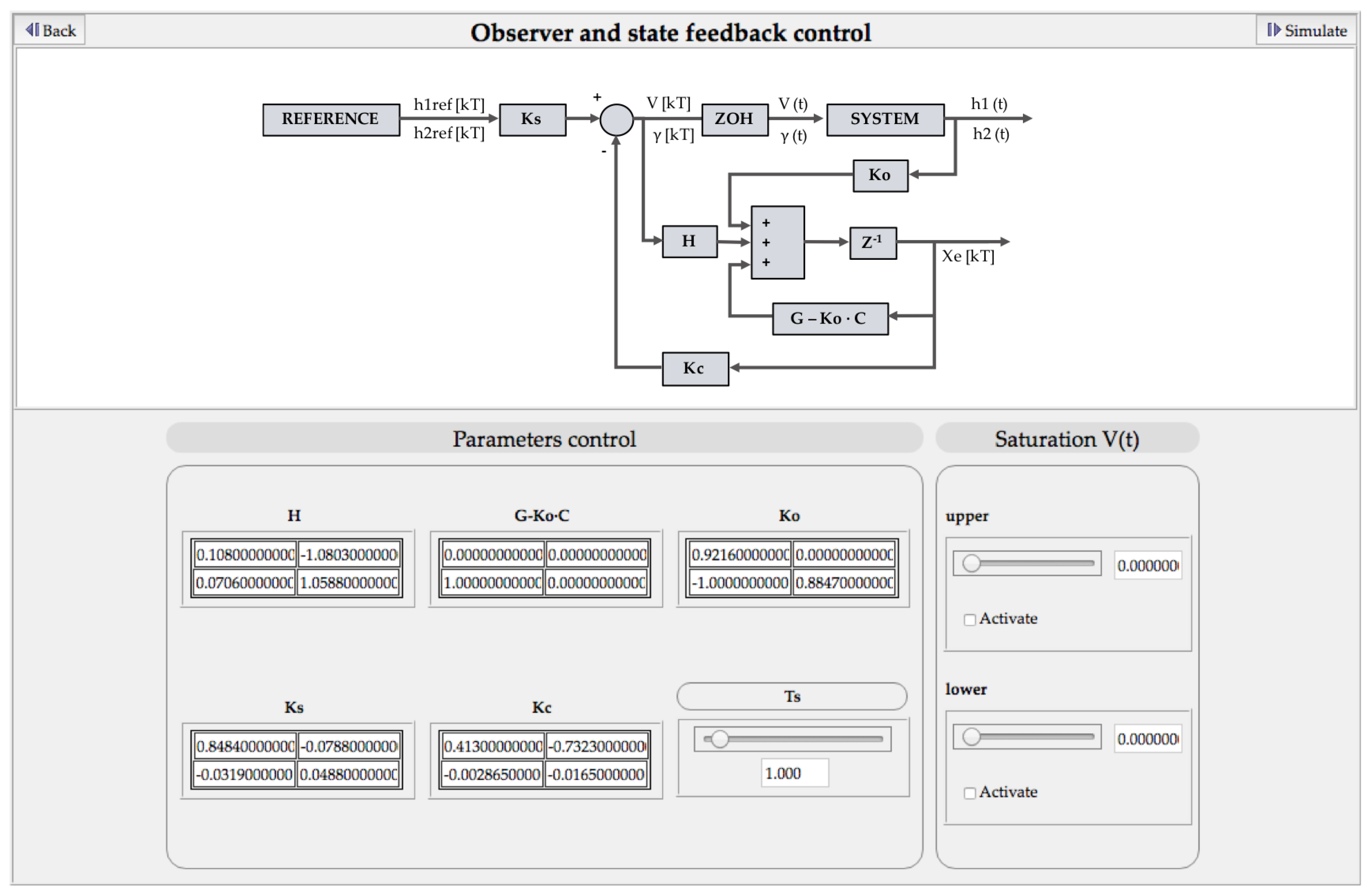
This subsection presents the modern theory control systems included in the platform, which are the main contribution of this paper along with the implementation of the discrete-time controllers using EJsS. The user can choose among: (a) state feedback; (b) observer and state feedback; and (c) integral controller, observer and state feedback control. To show the complete implementation, the steps for the deployment of the second option, whose block diagram is shown in Figure 3, is presented next as an example. However, all the possible combinations are available on the platform.

To implement the equations, it is essential to define all the parameters and variables beforehand. For this control, the parameters are the input matrix; a column matrix with two components ($B1$ and $B2$); the feedback matrix, whose size is 2 × 2 (components $r11$, $r12$, $r21$ and $r22$); the estimated state variables ($Xe1$ and $Xe2$); the observer matrix, with size 2 × 1 (components $Ko1$ and $Ko2$); the state feedback matrix, whose size is 1 × 2 (components $Kc1$ and $Kc2$); and an input gain (scalar $Ks$) to set the steady state.

4.2.1. Continuous-Time

In this kind of control, there are two differential equations (observer block), thus these are included on an ODE page (

Table 4. ODE page of the control through observed state feedback (SISO system).

State	Derivative
$\frac{dXe1}{dtime}$	$B1\ast q1\_inc+r11\ast Xe1+r12\ast Xe2+Ko1\ast h2\_inc$
$\frac{dXe2}{dtime}$	$B2\ast q1\_inc+r21\ast Xe1+r22\ast Xe2+Ko2\ast h2\_inc$

). The equation to obtain the control action is defined on a code page (Listing 10).

Listing 10. Code page: Continuous-time control through observed state feedback (SISO system).

q1_inc=(h2ref_inc*Ks) - ((Kc1*Xe1) + (Kc2*Xe2));

4.2.2. Discrete-Time

In this case, all equations of the controller must be described using code pages (Listing 11), including the equations that define the observer. Therefore, it is necessary to define two additional variables ($Xe1\_1$ and $Xe2\_1$), which are the estimated state variables in the next sampling instant. The estimated state variables ($Xe1$ and $Xe2$) will have the values of these ones in the next sampling instant.

Listing 11. Code page: Discrete-time control through observed state feedback (SISO system).

if ((Math.round(time/dt3))% (Ts3/dt3) === 0){

Xe1_1=(h2_inc*Ko1)+(q1_inc*H1)+(Xe1*r11)+(Xe2*r12);

Xe2_1=(h2_inc*Ko2)+(q1_inc*H2)+(Xe1*r21)+(Xe2*r22);

q1_inc=(h2ref_inc*Ks)-((Kc1*Xe1)+(Kc2*Xe2));

Xe1=Xe1_1;

Xe2=Xe2_1;

}

else{

Xe1=Xe1_1;

Xe2=Xe2_1;

q1_inc=q1_inc;

h2_inc=h2_inc;

}

5. Implementation of the Second Plant (MIMO System): Mathematical Model

Many physical systems have multiple inputs and/or multiple outputs. These are known as MIMO systems. This kind of system presents the complexity that an input variable can affect to several output variables. In advanced control subjects, students must learn how to control such systems and put these concepts into practice. For this reason, one of these systems has been implemented in the platform, so that the student can design several control systems and visualize the evolution of the controlled system. Section 5.1 describes succinctly this system. After that, the next subsections present the implementation of the equations of the system in EJsS. First, Section 5.2 details the steps for the linearized version, and then Section 5.3 for the original nonlinear model. Section 5.4 describes the implementation of the saturation block.

5.1. System Description

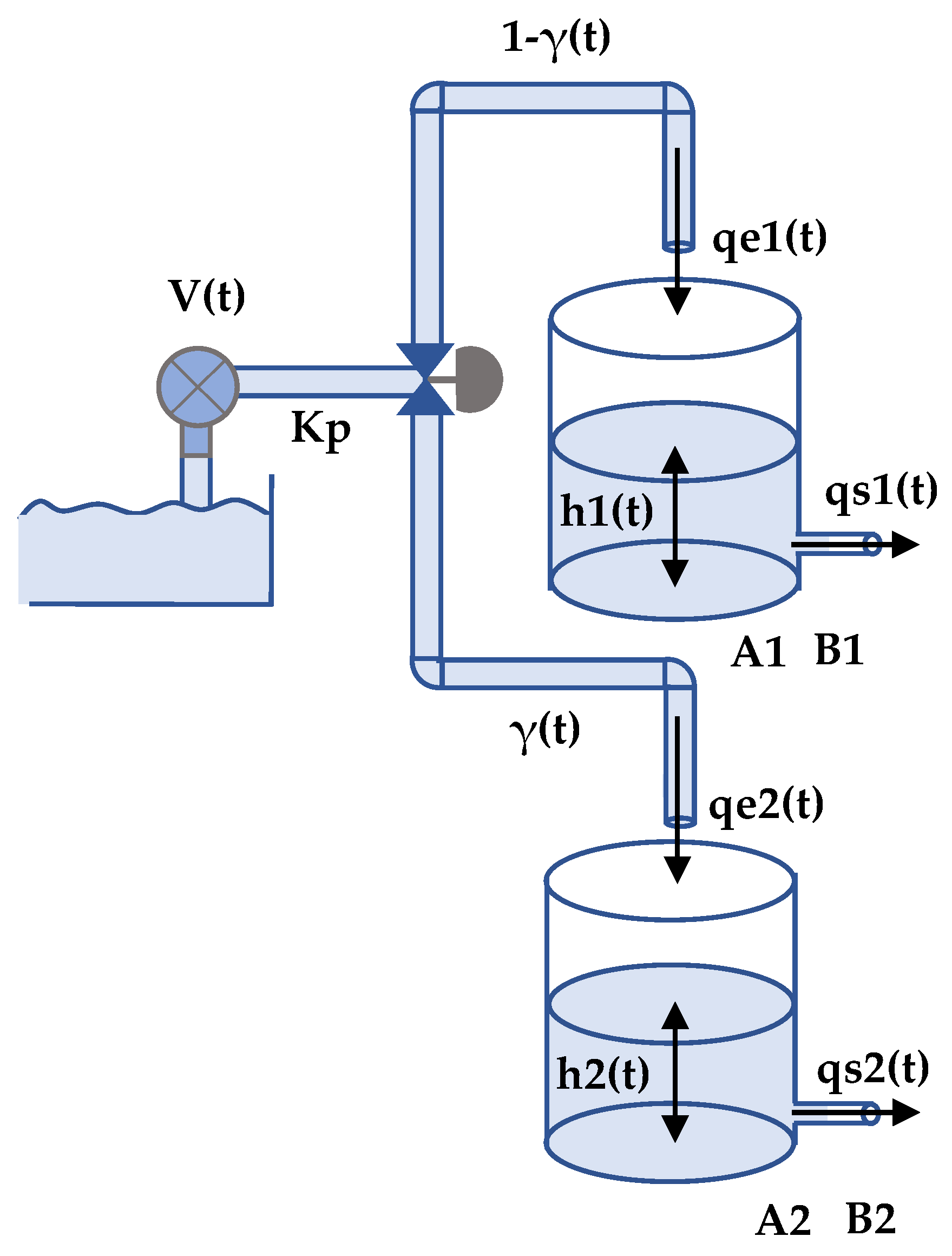
This plant consists of a valve and pump that distributes water to two tanks, as shown in Figure 4. The position of the valve determines how the flow from the pump is divided between both tanks.

The parameters of the process are the cross section of each tank ($A1$ and $A2$), the cross section of their respective outlet pipes ($B1$ and $B2$), the constant gain of the pump ($Kp$) and the acceleration of gravity (g).

On the other hand, the variables are the voltage applied to pump $V\left(t\right)$, the valve opening $\gamma \left(t\right)ϵ\left[0,1\right]$, the input flow to tank 1 $qe1\left(t\right)$, the output flow from the tank 1 $qs1\left(t\right)$, the input flow to tank 2 $qe2\left(t\right)$, output flow from the tank 2 $qs2\left(t\right)$ and the height of fluid in each tank $h1\left(t\right)$ and $h2\left(t\right)$. Once the parameters and variables are defined, the equations of this system are:

$$qe1\left(t\right)=Kp·V\left(t\right)·(1-\gamma (t\left)\right)$$

(5)

$$qe2\left(t\right)=Kp·V\left(t\right)·\gamma \left(t\right)$$

(6)

$$qs1\left(t\right)=B1·\sqrt{2·g·h1\left(t\right)}$$

(7)

$$qs2\left(t\right)=B2·\sqrt{2·g·h2\left(t\right)}$$

(8)

$$A1·\frac{dh1\left(t\right)}{dt}=qe1\left(t\right)-qs1\left(t\right)$$

(9)

$$A2·\frac{dh2\left(t\right)}{dt}=qe2\left(t\right)-qs2\left(t\right)$$

(10)

The input variables are the voltage $V\left(t\right)$ applied to the pump and the valve opening $\gamma \left(t\right)$. The variables to control are the fluid height of both tanks ($h1\left(t\right)$ and $h2\left(t\right)$). To obtain a linear state space representation, the equations must be linearized around a working point, since it is a nonlinear system. The codes to carry out the implementation of this system are shown in the next sections, with the purpose of easing the understanding of them, all variables and parameters that appear are defined in Appendix A.2.

5.2. Implementation of the Linearized Model

To begin with the implementation, it is necessary to declare the variables that appear in both the original and the linearized model (incremental variables), the value of the variables in the working point, the time variable and its differential. After that, the equations that define the behavior of the system must be implemented.

This subsection focuses on the linearized model that is obtained after linearizing the equations shown in Section 5.1. To implement it, the evolution and custom panel have been used.

The functions created are invoked by the ODE page, as shown in

Table 5. Differential equations of the linearized system (linear MIMO).

State	Derivative
$\frac{dh1\_inc}{dtime}$	$height1\_L(h1\_inc,gamma\_inc,V\_inc)$
$\frac{dh2\_inc}{dtime}$	$height2\_L(h2\_inc,gamma\_inc,V\_inc)$

, to calculate the first derivative of each state variable, using the Runge–Kutta method.

The height of fluid in each tank cannot be negative, thus the code implemented in these functions must test if it is happening as shown in Listings 12 and 13. In this case, the variables are incremental (case of the linearized model). Therefore, the value of the incremental height (h1_inc and h2_inc) could not be lower than the working point (h10 and h20) with negative sign.

Listing 12. Function to obtain the height of fluid in the first tank h1: height1_L (linear MIMO).

function height1_L (h1_inc, gamma_inc, V_inc) {

if(h1_inc<-h10){

h1_inc=-h10;

}

qe1_inc=-Kp*V0*gamma_inc+Kp*(1-gamma0)*V_inc; // input flow

qs1_inc=B1*Math.sqrt(g/(2*h10))*h1_inc; // output flow

return((1/A1)*(qe1_inc-qs1_inc));

}

Listing 13. Function to obtain the height of fluid in the second tank h2: height2_L (linear MIMO).

function height2_L (h2_inc, gamma_inc, V_inc) {

if(h2_inc<-h20){

h2_inc=-h20;

}

qe2_inc=-Kp*V0*gamma_inc+Kp*gamma0*V_inc;

qs2_inc=B2*Math.sqrt(g/(2*h20))*h2_inc;

return((1/A2)*(qe2_inc-qs2_inc));

}

Finally, the values of the variables are incremental and the evolution of some of them must be shown to the user, thus their value in the working point must be added to those variables, as shown in Listing 14.

Listing 14. Page code: Linearized system (linear MIMO).

h1=h1_inc+h10;

h2=h2_inc+h20;

gamma=gamma_inc+gamma0;

V=V_inc+V0;

5.3. Implementation of the Original Nonlinear Model

This model is implemented using an ODE page (

Table 6. Differential equations of the original system (nonlinear MIMO).

State	Derivative
$\frac{dh1}{dtime}$	$height1\_NL(h1,gamma,V)$
$\frac{dh2}{dtime}$	$height2\_NL(h2,gamma,V)$

) to solve the continuous-time differential equations, as well as a function for each state variable (Listings 15 and 16), which will be invoked by the ODE page.

The code implemented in each function computes the corresponding first derivative by means of the equations shown in Section 5.1, as can be seen in Listings 15 and 16.

Listing 15. Function to obtain the height of fluid in the first tank h1: height1_NL (nonlinear MIMO).

function height1_NL (h1, gamma, V) {

if (h1<0){

h1=0;

}

qe1=Kp*V*(1-gamma);

qs1=B1*Math.sqrt(2*g*h1);

h1_d=(1/A1)*(qe1-qs1); //save the first derivative value of h1

h1_inc=h1-h10; // compute the incremental value of h1

return((1/A1)*(qe1-qs1));

}

Listing 16. Function to obtain the height of of fluid in the second tank h2: height2_NL (nonlinear MIMO).

function height2_NL (h2,gamma,V) {

if (h2<0){

h2=0;

}

qe2=Kp*V*gamma;

qs2=B2*Math.sqrt(2*g*h2);

h2_d=(1/A2)*(qe2-qs2); //save the first derivative value of h2

h2_inc=h2-h20; // compute the incremental value of h2

return((1/A2)*(qe2-qs2));

}

5.4. Saturation

As mentioned above, sometimes the values of the control action are limited in the real plant. For example, the valve opening $\gamma \left(t\right)$ can only take values between 0 and 1 in this plant, thus a saturation block has been created to this variable. In addition, the saturation of the pump voltage is implemented, but, in this case, it will only be active when the student determines it. Therefore, he/she must introduce the upper and/or lower limit values.

This part has been included as code on each page created for the different types of control. As can be seen in Listing 17, two boolean variables (sat_V_upper and sat_V_low) have been created to indicate if the upper and/or lower saturation of the pump voltage is activated.

Listing 17. Code page: Saturation block (MIMO).

// valve constant (gamma) saturation

if (gamma_inc+gamma0 > value_gamma_sat_upper){

gamma_inc=value_gamma_sat_upper-gamma0;

}

if (gamma_inc+gamma0 < value_gamma_sat_low){

gamma_inc=value_gamma_sat_low-gamma0;

}

// voltage applied to pump (V) saturation

if (sat_V_upper){

if (V_inc+V0 > value_V_sat_upper){

V_inc=value_V_sat_upper-V0;

}

}

if(sat_V_low){

if(V_inc+V0 < value_V_sat_low){

V_inc=value_V_sat_low-V0;

}

}

6. Implementation of the Second Plant (MIMO System): Controllers

Several kinds of control techniques have been included in this simulation software, in this case to control a virtual MIMO system. The user can choose between techniques based on classic and on modern theory. This section describes how the controllers are implemented in EJsS. More information about the implementation of the controllers can be found in [21,31].

Section 6.1 focuses on the implementation of the controllers based on classical theory (continuous-/discrete-time) and Section 6.2 describes the implementation of the controllers based on modern theory (continuous-/discrete-time).

6.1. Classical Control Theory

This subsection, as mentioned above, presents the implementation of the PID controller. This kind of controller works in closed-loop, thus its input is the error signal. The product of this signal and a gain $Kp$ represents the proportional part. On the other hand, the derivative of the error signal times a gain $Kd$ is the derivative part. Finally, the product of the integral of the error and a gain $Ki$ represents the integral part. The output of the PID controller is the addition of all these parts.

To begin with its implementation, it is necessary to define the proportional ($kp1$ and $kp2$), derivative ($kd1$ and $kd2$) and integral ($ki1$ and $ki2$) constants, as well as the error signal ($error$), its derivative ($derror$) and integral ($ei$), and all variables that allow us to describe behavior of this kind of controller. All these variables are included on the page of variables.

6.1.1. Continuous-Time

The integral part of the controller has been defined on an ODE page (

Table 7. ODE page of classical control (MIMO system).

State	Derivative
$\frac{dei\_1}{dtime}$	$error1$
$\frac{dei\_2}{dtime}$	$error2$

), since it has been expressed as a differential equation considering that the derivative and integral are inverse operations.

By contrast, the rest of the necessary equations are defined on a code page (Listing 18) corresponding to this type of control. The derivative of each error signal is equal to the derivative of its corresponding state variable with negative sign, since the incremental reference values are considered constant. In this platform, the values of these variables (h1_d and h2_d) are assigned every time that the functions are invoked. This is due to the fact that their values depend on the model being used.

Listing 18. Code page: Continuous-time PID controller (MIMO system).

error1=h1ref_inc-h1_inc;

error2=h2ref_inc-h2_inc;

derror1=-h1_d; // first derivative value of h1

derror2=-h2_d; // first derivative value of h2

V_inc=kp1*error1+ki1*ei1+kd1*derror1;

gamma_inc=kp2*error2+ki2*ei2+kd2*derror2;

6.1.2. Discrete-Time

In this case, all the equations which are necessary to implement the controller are included on a code page (Listing 19). These equations will only be run when the simulation time is equal to a sampling instant.

Listing 19. Code page: Discrete-time PID controller (MIMO system).

if ((Math.round(time/dt))% (Ts/dt) === 0){

//Derivative

derror1=(h1ref_inc-h1_inc)-error1;

derror2=(h2ref_inc-h2_inc)-error2;

//Proportional

error1=h1ref_inc-h1_inc;

error2=h2ref_inc-h2_inc;

//Integral

ei1=error1+ei1;

ei2=error2+ei2;

V_inc=kp1*error1+ki1*ei1+kd1*derror1;

gamma_inc=kp2*error2+ki2*ei2+kd2*derror2;

}

else{

V_inc=V_inc;

gamma_inc=gamma_inc;

derror1=derror1;

derror2=derror2;

error1=error1;

error2=error2;

ei1=ei1;

ei2=ei2;

}

6.2. Modern Control Theory

This subsection presents the modern control systems included in the platform. The MIMO plant can be controlled using one of the next options: (a) state feedback; (b) observer and state feedback; and (c) integral controller, observer and state feedback control. All of them are included in the simulation software, however, in this paper, only the implementation of the second option is shown. To begin, the parameters and the variables of this control must be defined, as the input matrix $\left[B11,B12;B21,B22\right]$, the feedback matrix $\left[r11,r12;r21,r22\right]$, the estimated state variables $\left[Xe1;Xe2\right]$, the observer matrix $\left[Ko11,Ko12;Ko21,Ko22\right]$, the state feedback matrix $\left[Kc11,Kc12;Kc21,Kc22\right]$ and the steady gain matrix $\left[Ks11,Ks12;Ks21,Ks22\right]$. Additionally, the equations that describe the behavior of the controller must be defined. However, the way to implement them depends on the kind of control: continuous-time or discrete-time, as described in the next subsections.

6.2.1. Continuous-Time

In this type of control, there are two differential equations belonging to the observer part, which are used to calculate the estimated state variables. These equations have been defined on an ODE page, as shown in

Table 8. ODE page of discrete observer state feedback control (MIMO system).

State	Derivative
$\frac{dXe1}{dtime}$	$(B11\ast V\_inc+B12\ast gamma\_inc)+(r11\ast Xe1)+(r12\ast Xe2)+(Ko11\ast h1\_inc+Ko12\ast h2\_inc)$
$\frac{dXe2}{dtime}$	$(B21\ast V\_inc+B22\ast gamma\_inc)+(r21\ast Xe1)+(r22\ast Xe2)+(Ko21\ast h1\_inc+Ko22\ast h2\_inc)$

. By contrast, the equations to calculate the control action are included on a code page, whose implementation can be seen in Listing 20.

Listing 20. Code page: Observer state feedback control (MIMO system).

V_inc=(Ks11*h1ref_inc)+(Ks12*h2ref_inc)-(Kc11*Xe1+Kc12*Xe2);

gamma_inc=Ks21*h1ref_inc+Ks22*h2ref_inc-Kc21*Xe1+Kc22*Xe2;

6.2.2. Discrete-Time

The implementation of this discrete-time controller is carried out on a code page, as already mentioned for the previous plant. This code can be seen in Listing 21.

Listing 21. Code page: Discrete observer state feedback control (MIMO system).

if ((Math.round(time/dt3))% (Ts3/dt3) === 0){

V_inc=(Ks11*h1ref_inc)+(Ks12*h2ref_inc)-(Kc11*Xe1+Kc12*Xe2);

gamma_inc=(Ks21*h1ref_inc)+(Ks22*h2ref_inc)-(Kc21*Xe1+Kc22*Xe2);

//first derivative value of the first estimated state

Xe1_1=(H11*V_inc+H12*gamma_inc)+(r11*Xe1)+(r12*Xe2)+(Ko11*h1_inc+Ko12*h2_inc);

//first derivative value of the second estimated state

Xe2_1=(H21*V_inc+H22*gamma_inc)+(r21*Xe1)+(r22*Xe2)+(Ko21*h1_inc+Ko22*h2_inc);

// save these values

Xe1=Xe1_1;

Xe2=Xe2_1;

}

else{

Xe1=Xe1_1;

Xe2=Xe2_1;

gamma_inc=gamma_inc;

V_inc=V_inc;

h1_inc=h1_inc;

h2_inc=h2_inc;

}

7. Results of the Simulation

This section explains how the HTML pages created must be used. In addition, results obtained with both the linearized and the original model are shown. The system selected to perform this analysis is the MIMO system controlled discrete-time.

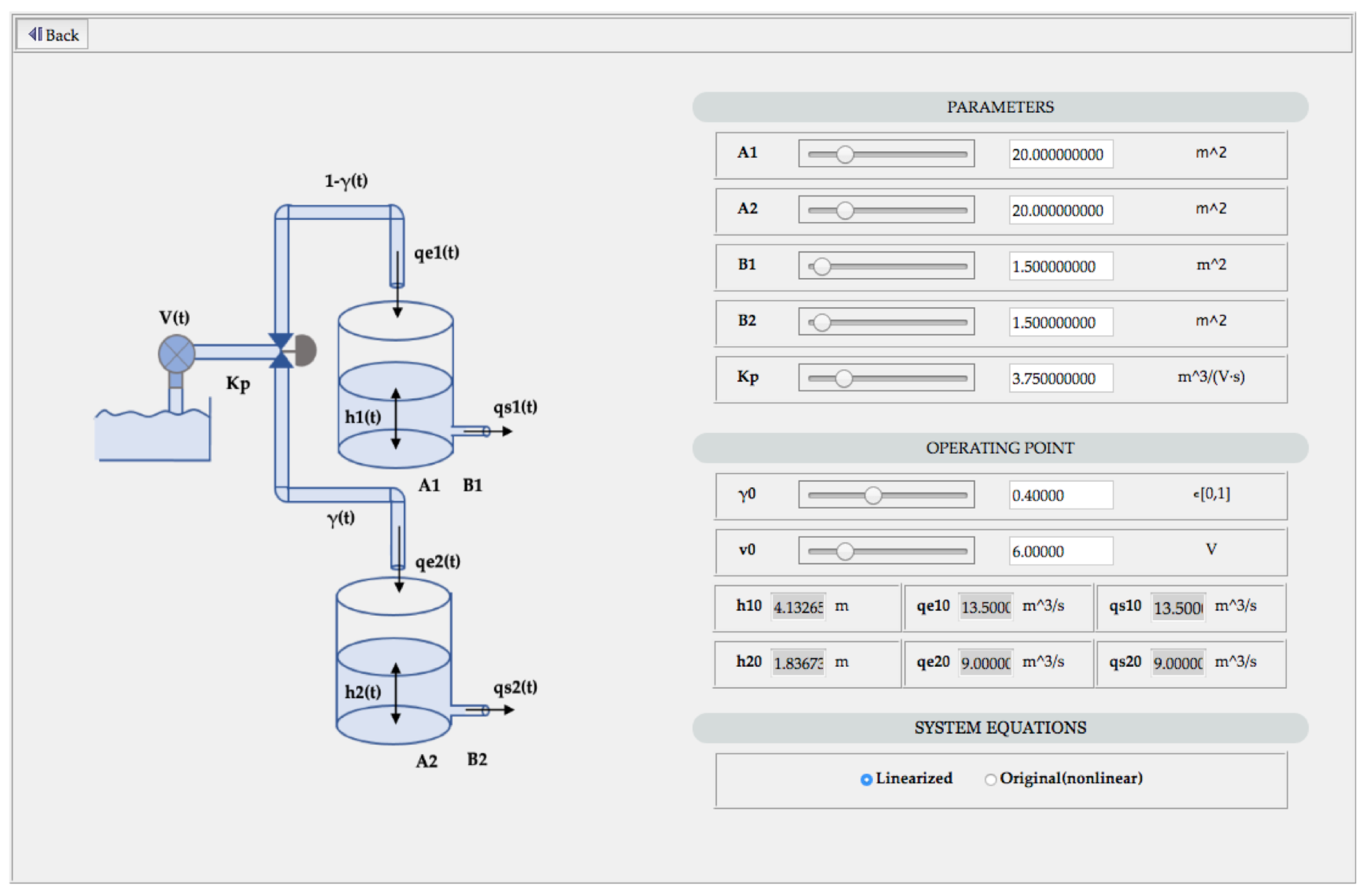
Firstly, the student will see a main window which includes an image of the system, a menu and a title indicating if the control is continuous- or discrete-time. There are several options in the menu: (a) parameters; (b) classic control; or (c) state-space control. The user will select the first one (Figure 5) to define the values of each parameter, as well as the working point. In addition, the model to be used in the simulation (linearized or original equations) can be selected here.

In this window, the user can choose the type of control, for instance state-space control choosing between state feedback control, observer and state feedback control or integral controller, observer and state feedback control. In this article, the second option has been selected. Once the controller has been chosen, the user must calculate the parameters of this control, so the response of the system meets determined specifications.

To design the controller, the user must linearize the system around the working point introduced, and obtain the state space representation. After that, it must be discretized with a specific sampling time and considering a zero-order hold. Finally, the parameters values must be calculated and introduced in the window of the selected controller, as shown in Figure 6. In the top of this window, there is a button at left for going back to the menu and another at the left which permits accessing the simulation window. The control schema is visualized in the center and the student must write the value of all parameters at the bottom of this window.

In this case, these parameters are the state feedback matrix $Kc$, the matrices of the observer ($Ko$, H, $G-Ko·C$) and the input gain matrix Ks. Besides, the sample time must be introduced since the controller is discrete-time.

On the other hand, there is an optional block corresponding to the voltage saturation of the pump $V\left(t\right)$. The user can determine the maximum and minimum values of the control action signal and activate the saturation by means of a selector.

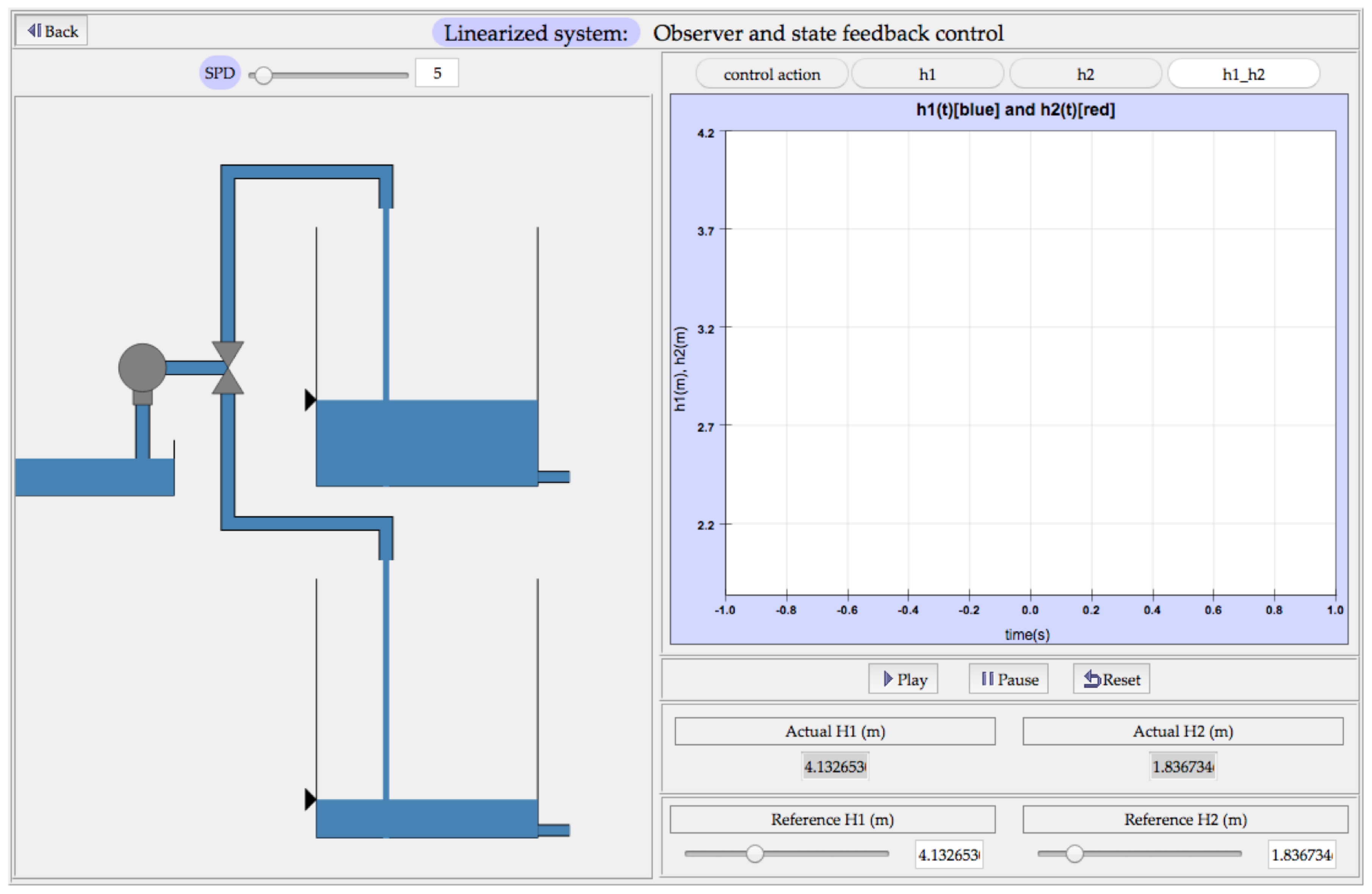
The next step is to click on the “simulate” button. In the right half of this window, the evolution of some relevant variables can be observed through drawing elements (Figure 7). In addition, there is a slider and a parsed field, which permits changing the SPD (Steps Per Display) value. The user can increase its value with the purpose that the system could advance multiple times before the visualization is redrawn. On the left half, there are four buttons to choose the variables which will be visualized, a graphic that shows the evolution of the selected variable and a set of buttons (play, pause and reset).

On the bottom of this screen, the user can introduce the reference value of each output and their values are shown versus the simulation time. After that, the play button must be clicked for the simulation start.

The reset button must be clicked if we want the value of each variable to be set to its initial value. The back button does this as well, but also returns to the menu.

On the platform website [29], the student can find more information about this simulation software, and also some laboratory guides where all steps are described to take advantage of this tool. In addition, some guidelines to calculate each controller are included. First, the user is proposed to follow these steps with a set of default parameters and, once he/she knows how use it, there are proposed a variety of exercises, thus the student calculates the parameters of each controller and then he/she simulates it in the tool and checks the performance of the controlled system.

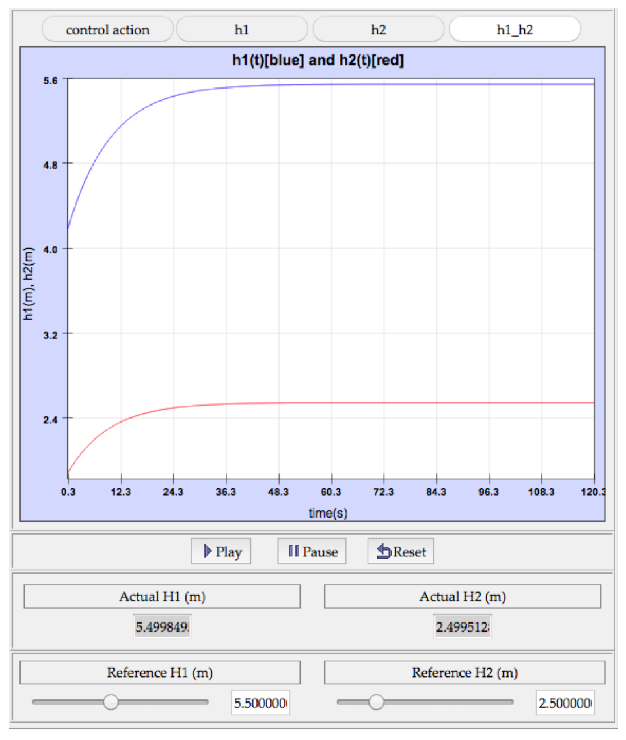
In this example, the system is controlled using the observer and state feedback control, whose parameters are shown in Figure 6 (default values). The user introduces a value of 5.5 m for the H1 reference and 2.5 for the H2 reference. Subsequently, the behavior of the system is shown in Figure 8.

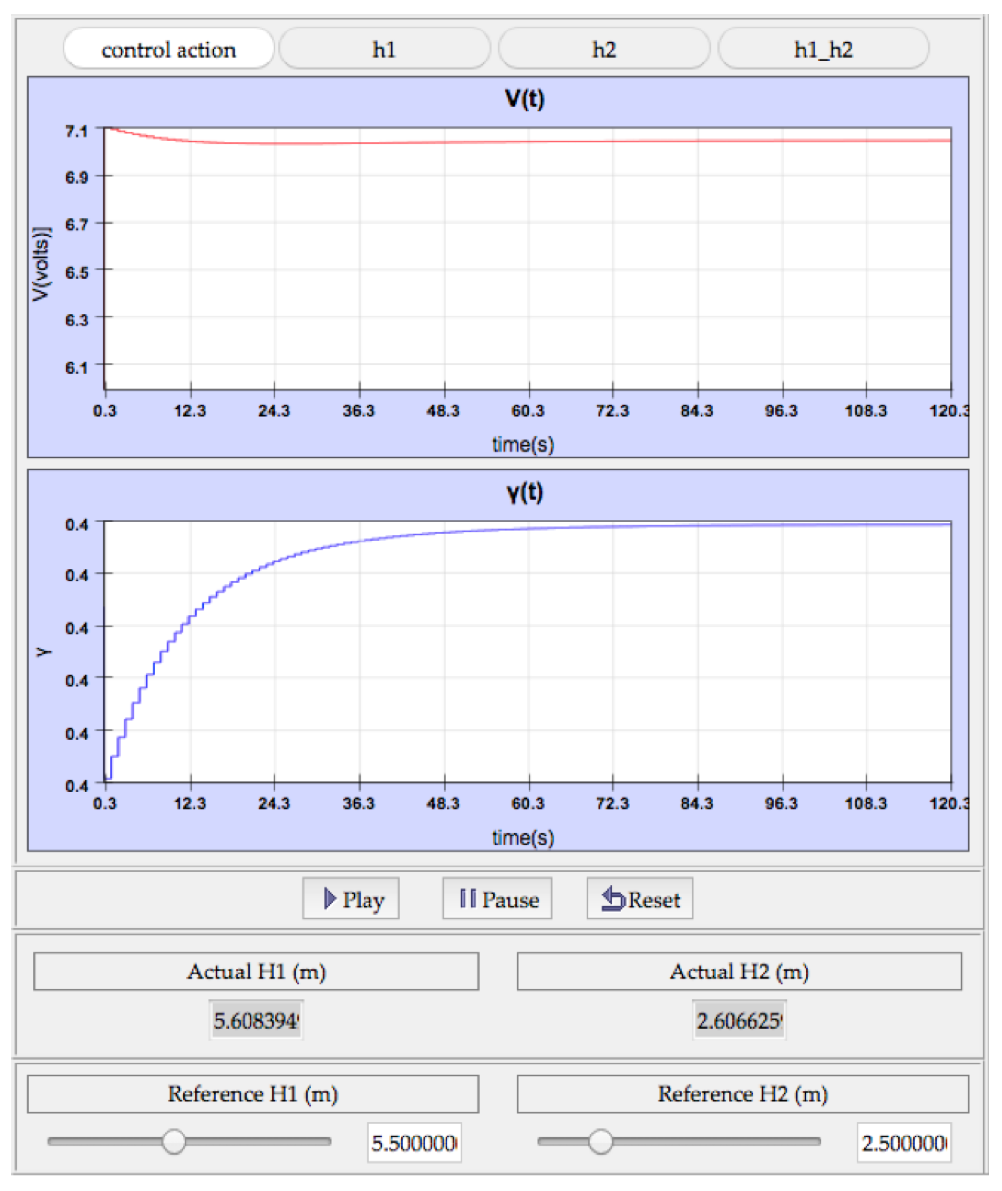
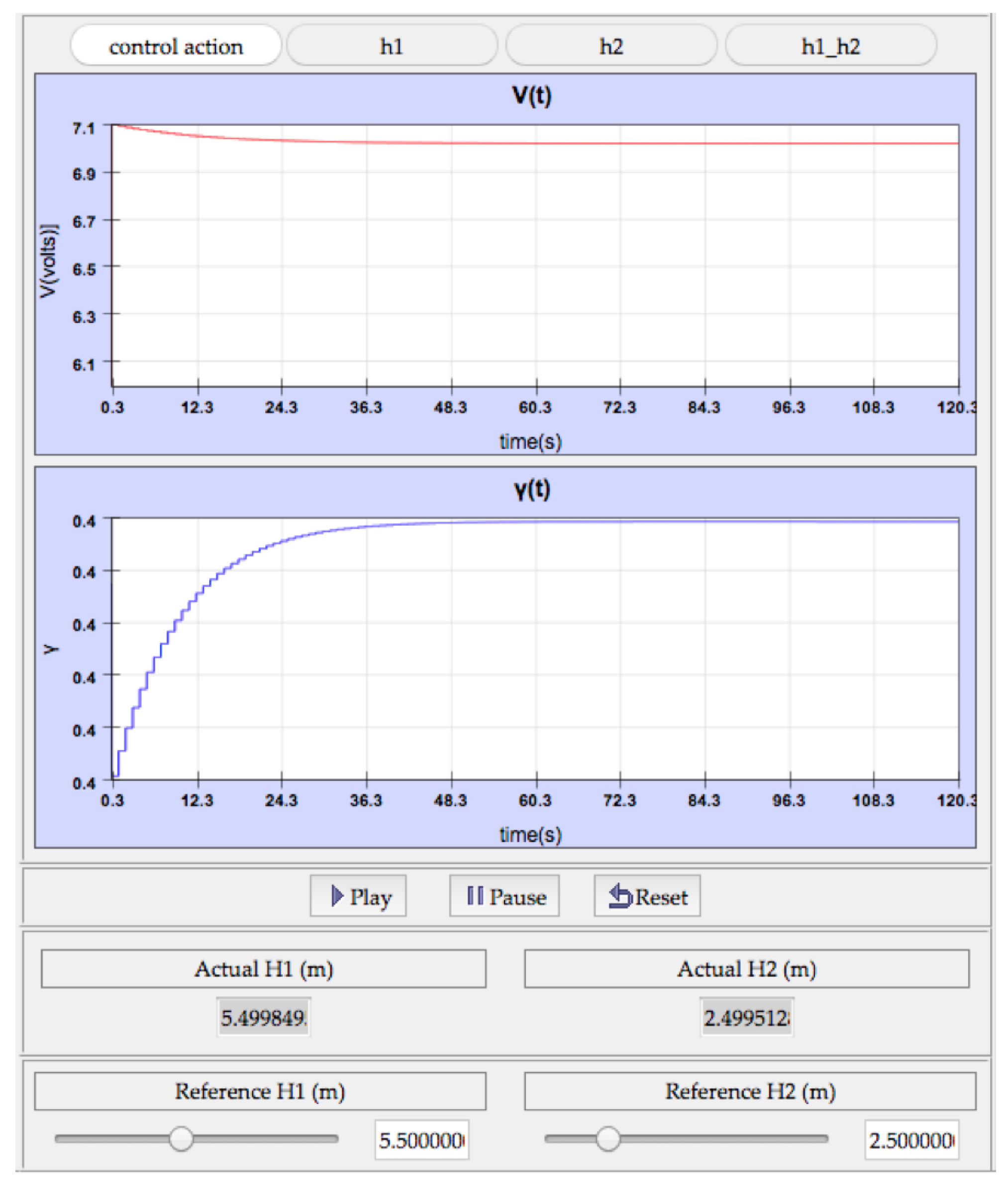
The user can change the graphic using the buttons on the top, with the purpose of visualizing the evolution of the variable that he/she wants. The available options are the control action signals (Figure 9) and the evolution of the outputs separately or in the same graphic.

Thus far, the student has been able to observe if the controller designed works correctly for the linearized model. In this example, both heights (the outputs of the system) stabilize for the reference values introduced. As discussed in this article, the student will also be able to see if the same happens with the original (nonlinear) model.

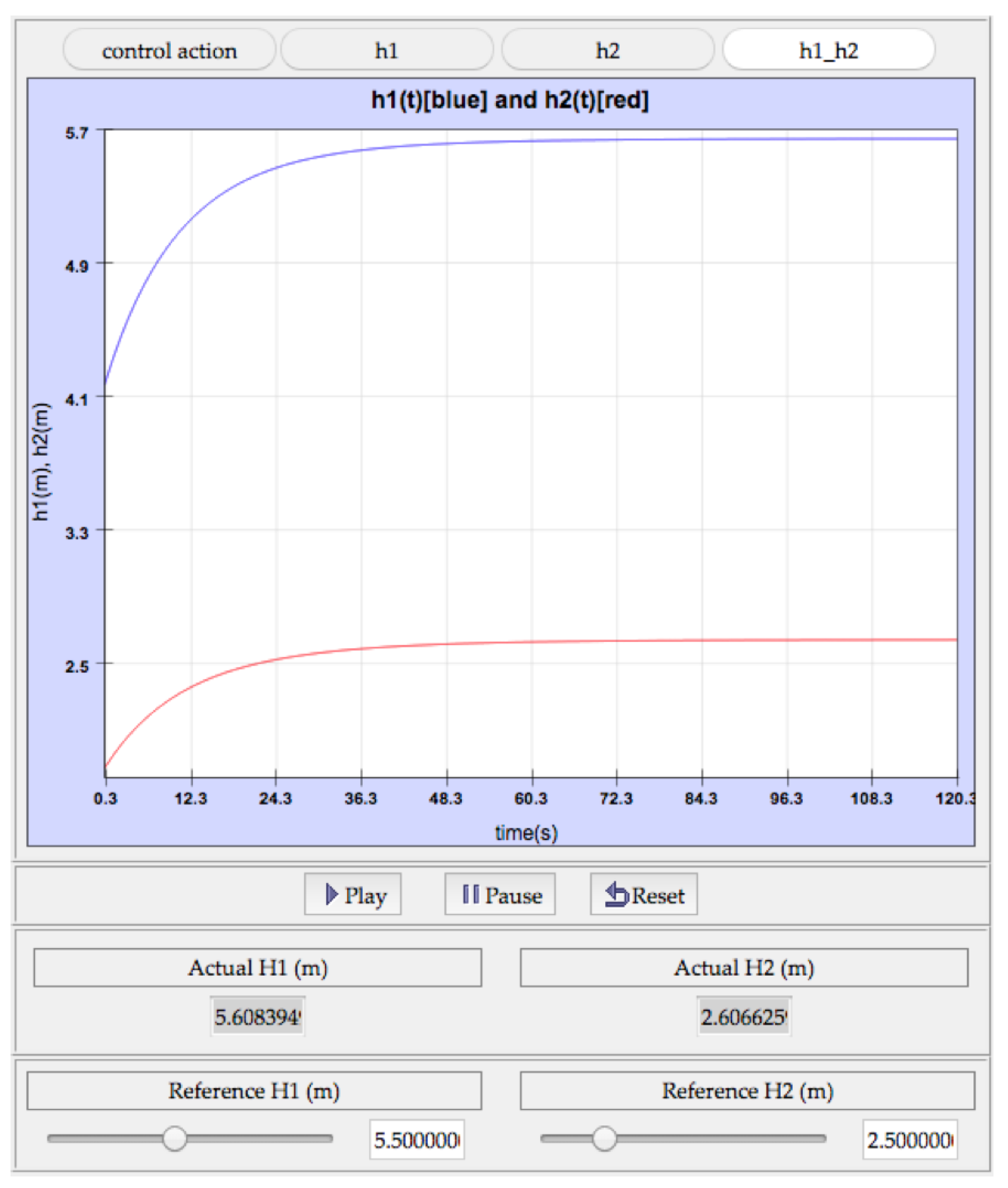
For comparative purposes, Figure 10 shows the evolution of the output when the same controller is used, considering the equations of the original (nonlinear) plant. Figure 11 shows the evolution of the control action in this case. Comparing the output responses of either model, both are very similar, as well as the behavior of the control actions (Figure 11). However, the final values of the heights do not agree with the reference values introduced, although the system does stabilize with a near value. It happens because the nonlinear model works correctly in a short range around the operating point; in other words, away from it the difference between the behavior of linearized and nonlinear model is greater.

This kind of experiments results greatly illustrative for the students and, after them, they can use the platform to check how the addition of the integral controller solves this issue.

Therefore, the student has put into practice the concepts of control systems after following all steps. First, he/she has identified and modeled two nonlinear systems. Then, the student has designed a controller based on classical and modern control theory, and after that the control system has been simulated. The designed controller has been applied to the linearized and nonlinear model, thus the student has been able to see the difference between an ideal and the real plant.

8. Conclusions

The purpose of this article is to present a simulation software, in which the student can design a controller and check the behavior of the controlled system. Both a SISO and a MIMO plant have been included, which are hydraulic and nonlinear. Due to this characteristic, both models (linearized and original equations) have been implemented so that the student can observe how the linearized model behaves using the calculated control, and what happens if that control is applied to the original model of the system.

The control system can be carried out continuous- or discrete-time, so for each system two HTML pages have been created: (a) SISO system controlled using a continuous-time controller; (b) SISO system controlled using a discrete-time controller; (c) MIMO system controlled using a continuous-time controller; and (d) MIMO system controlled discrete-time. In brief, there are four modules, thus other studies can focus on the part which interests them. To access these HTML pages, the user must enter the website [29]. In addition, there is one laboratory guide by module. All steps are shown to model the system and to design the controller, as well as how the simulation software must be used.

The implementation of the linearized and original model, as well as the different types of continuous-time and discrete-time controllers, have been explained step by step through out this article.

This simulation software permits the student to design and test several types of control systems, based on classical and modern control theory. Besides, he/she can configure the system and controller parameters. Finally, the behavior of the controlled system (linear and original model) is shown. The objective of this tool is to help students, so that they can experience the theory concepts studied in classroom.

EJsS has turned out to be a complete tool to implement all required modules in an intuitive manner. It presents enough resources both to design the interface for simulations and to obtain the evolution of the physical system based on its equations, either continuous-time or discrete-time. All modules implemented are at the disposal of the scientific community so that they can reuse them in future implementations of physical system laboratories.

There are some possible improvements of the platform that are under consideration. First, additional plants could be implemented, for example mechanical or electric systems. In addition, more complex and higher-order hydraulic plants can be added, such as a plant composed by four tanks in which the height of each one is controlled. In addition, other control approaches could be included, for instance optimal, adaptive and fuzzy control.