A Dynamic Bayesian Network for Vehicle Maneuver Prediction in Highway Driving Scenarios: Framework and Verification

Abstract

Accurate maneuver prediction for surrounding vehicles enables intelligent vehicles to make safe and socially compliant decisions in advance, thus improving the safety and comfort of the driving. The main contribution of this paper is proposing a practical, high-performance, and low-cost maneuver-prediction approach for intelligent vehicles. Our approach is based on a dynamic Bayesian network, which exploits multiple predictive features, namely, historical states of predicting vehicles, road structures, as well as traffic interactions for inferring the probability of each maneuver. The paper also presents algorithms of feature extraction for the network. Our approach is verified on real traffic data in large-scale publicly available datasets. The results show that our approach can recognize the lane-change maneuvers with an F1 score of 80% and an advanced prediction time of 3.75 s, which greatly improves the performance on prediction compared to other baseline approaches.

1. Introduction

Intelligent vehicles are promising tools for future transportation. They show an enormous potential to improve driving safety and the efficiency of transportation systems. However, current technologies on intelligent vehicles still have limitations, especially when they are driving in complex dynamic environments. The limitations lie in making socially compliant maneuvers and completely avoiding collisions with dynamic obstacles (surrounding vehicles and other moving traffic participants). To overcome these limitations, intelligent vehicles should gain a better understanding of dynamic surroundings.

There are many previous studies concerning the understanding of dynamic surroundings. Intelligent vehicles normally use onboard sensors, such as digital cameras, depth cameras, LIDARs, and radar ([1,2,3,4,5,6]) for accurate detection of dynamic surroundings. Inspired by human drivers, who have an inherent capacity to anticipate the future traffic, people try to enable intelligent vehicles to predict the future motion of surrounding vehicles. The prediction helps intelligent vehicles make safe and socially compliant decisions in advance [7,8], thus guarantee the driving safety without losing too much comfort or being too conservative.

However, accurate motion prediction is an extremely challenging task because there exists a large number of potential factors that can influence the predicted results. For instance, the sensors installed on an intelligent vehicle may not detect all cars in the neighborhood due to limited visibility and occlusion. Moreover, different driving habits of human drivers will also increase the difficulty of the motion prediction. According to [9], predicting maneuvers is essential and significant for reliable motion prediction, in that maneuvers reflect social conventions and long-term trends of a rational driving.

While maneuver prediction of surrounding vehicles received widespread attention in the past three years, most state-of-the-art approaches do not apparently show excellent predictive performance. Besides that, some reported approaches are only verified in a simulation environment or small self-collected datasets, which leads to difficulties to assess their performance on prediction.

Contribution

In contrast, this paper proposes a practical, high-performance, and lost-cost maneuver-prediction approach. Moreover, our approach is verified on large-scale and publicly available real-traffic datasets instead of using small self-collected datasets. The main features of this paper include three aspects.

(1) Practicality

Our prediction approach is based on a dynamic Bayesian network (DBN). (i) The probabilistic framework can effectively deal with the uncertainties in the prediction. The uncertainties are often faced by intelligent vehicles because of limited sensing capacity of sensors and changing environments. (ii) Moreover, our approach is more flexible to be extended to other scenarios compared to the approaches using hand-designed rules. In other words, though the predicted scenario in this paper focuses on the lane-change maneuver prediction in highways, the DBN can be extended to other scenes, for example anticipating maneuvers of turning to a crossroad. (iii) Besides, the DBN is intuitive to add predictive features based on the causal relationship in different predicting scenarios.

(2) High performance

Our approach adopts more features relatively compared to traditional approaches using a unique feature. The features we used reflect not only the physical states and road information but also traffic interactions. Meanwhile, the DBN considers the continuous changes and historical states of the chosen features. The experimental results show that our approach gains comparable prediction performance compared to other benchmark approaches.

(3) Low cost

Our approach needs less computational resource compared to the one using deep neural networks for prediction.

The remainder of the paper is organized as follows. In Section 2, the state-of-the-art techniques of maneuver prediction for surrounding vehicles are compared and classified based on predictive features. In Section 3, the framework of our system is introduced. In Section 4, the multi-dimensional predictive features and the structure of our DBN for maneuver prediction are discussed. In Section 5, the algorithm for feature extraction and the qualitative discretization method are highlighted. In Section 6, the datasets we applied are introduced, and the optimal parameters for discretization are selected. Moreover, the prediction performance of the proposed approach is compared with other state-of-the-art benchmark approaches. Finally, Section 7 concludes and suggests future work.

2. State of the Art

The predictive features are crucial in the fields of pattern recognition [10,11,12]. The existing approaches to maneuver prediction can be classified based on their used predictive features. Generally, commonly used features for maneuver prediction can be classified into three types: (1) features related to physical states of vehicles, (2) features related to road structures, (3) features related to traffic interactions. The specific comparison is shown in

Table 1. Comparative review of approaches on intention recognition for surrounding vehicles.

Applied Features		Approaches
Unique	Physics related	motion model [13,14], intelligent driver model [15], prototype trajectory set [16]
	Road structure-related	set-based prediction [17,18]
Multiple	Without traffic interaction (combined the physics and road structure)	naive Bayesian approach [19], rule-based approach [20], decision tree-based approach [21], interacting multiple model filter [22,23], hidden Markov model [24,25,26]
	With traffic interaction	convolutional neural network [27], long short-term memory network [28,29,30], interactive hidden Markov model [31], Bayesian network and its variations [32,33,34,35,36]

and will be discussed in the following of this section.

Physics-based features mainly refer to detective states (e.g., position, velocity, acceleration) of surrounding vehicles. Because the motion of vehicles satisfies kinematic and dynamic laws, the historical states of vehicles with kinematic and dynamic laws can be used to infer possible future states (i.e., motion boundaries) of vehicles. Traditional physics-based prediction approaches use a motion model based on constant velocity (CV), constant acceleration (CA), constant turn rate (CTR) or their combinations (e.g., [13]). An intelligent driver model (IDM), which explicitly builds the relationship between maneuvers at intersections and velocity, acceleration of predicting vehicles, is proposed in [15]. Some of these approaches assume Gaussian noise existing in the detection of states, thus improving the ability to handle uncertainties. Contrarily, some approaches do not assume a specific distribution of the noise. For example, in [14], the Markov chains and Monte Carlo method are used to predict the probabilistic occupancy and furthermore determining the collision risk. Moreover, [16] presents an approach based on a set of trajectory prototype. The trajectory set is collected from fixed driving scenarios. The maneuver is predicted by comparing the historical trajectory and prototypes using similarity metrics. Though this approach can gain a relatively high performance in fixed driving scenarios, it is hard to be adaptive to other traffic situations. In general, physics-based prediction approaches are always limited to short-term prediction, since uncertainties not only come from the detection of states but also the driving environments and traffic interactions. These external features also influence driving maneuvers.

Road structure-based features mainly refer to road topology (which can be seen as a simplified road representation), road signs, and traffic rules. The typical road structure-based prediction approaches include [17,18,37]. In [17,18], a set-based approach is presented, which uses a geometric graph to represent roads. The approach is expected to work in arbitrary road networks and guarantee the collision-free reachability analysis. However, the prediction generates an over-approximate occupancy, which is too conservative to provide enough information for the motion planning of intelligent vehicles. In [37], the features considering traffic rules are discussed. However, the hand-designed rules are too complex to be modeled. The simulation and verification are also hard to perform.

Recently, many prediction approaches combine physics-based features and road structure-based features. In [19], the conditional probability of features is modeled as a Gaussian mixture model. Then, the approach applies a naive Bayesian method to classify the lane-change maneuver. Moreover, the predictive power of all features is compared, and thereby obtaining features with maximum predictive power. Compared with the approaches which use only physics-based features, the predicting accuracy of the approach has been remarkably improved. In [20], maneuver prediction is performed based on two types of features and ontology-based rules, which models priori driving knowledge. Similarly, the paper [21] adopts the decision tree method for predicting risk behaviors in cut-in scenes. However, these two methods [20,21] have high complexity and are difficult to be extended to other environments. In [22], a unified multi-model filtering algorithm for maneuver prediction and trajectory prediction is proposed. The approach uses a reference path to help extract the road-structure related features. However, the predicted results seem effective only in short term. In [25], a hidden Markov model (HMM) is used to predict lane-change maneuvers. It is announced to achieve 96% accuracy, without reporting the false warning rate.

Interaction-aware features predict trajectories of surrounding vehicles with consideration of the dependencies between vehicles. The features represent how the motion is influenced by the traffic interaction (e.g., collision avoidance, social conventions), therefore interaction-aware prediction approaches own a better understanding of the whole future traffic situation. Although the interaction-aware features are essential in maneuver prediction, there are few approaches effectively considering these features before 2014 according to the review literature [9]. In the past three years, increasing researches use these features implicitly or explicitly. With the development of deep learning technology, approaches based on the deep learning framework (e.g., [27,28]) can model interactions implicitly. In [27], a Convolution Neural Network (CNN) is modeled to predict the lane-change maneuver. In [28], a Long Short-Term Memory (LSTM) network shows a promising performance on predicting predefined maneuvers (i.e., turning left, turning right, and keeping straight) at intersections. Even though these approaches can model the interaction implicitly, the neural network model is not intuitive in the prediction process. Moreover, the high computational resource and large training data are required.

Thus, the explicit interaction-aware prediction approaches are proposed. In [31], the maneuver prediction is based on an optimization approach, whose objective function models the interactions of surrounding vehicles. The Bayesian network and its variants [32,33,34,35,36] are common to model the interactions explicitly. In [32], an object-oriented Bayesian network (OOBN) is employed to predict lane-change maneuvers, which attempts to be adaptive to different scenarios. In [33], a DBN models driving intention of all vehicles instead of each separate vehicle, but the conditional distribution in the network requires a large number of parameter settings and model assumptions. In [34], a Bayesian network is established to predict maneuvers in highways. However, the network does not consider dynamic changes, leading to poor predicting performance. Besides, as the paper mainly focuses on the analysis of collision risks, the prediction performance is unverified. In [35], interactions are modeled through model-based cost functions, which requires expert knowledge. The result of the model is then used as a priori knowledge of the Bayesian network to simplify network structure. Unlike our network, all previously mentioned networks lack either full consideration of predictive features or capabilities in producing continuous predictions.

3. System Architecture

The architecture of our maneuver-prediction system is shown in Figure 1. The core of our system is a DBN with the three-layer structure, which fully considers the predictive features and the relevance of continuous maneuvers. The network is instantiated for each surrounding vehicle. For simplicity, each node of the DBN represents one layer in a one-time step in the figure.

After we have determined the structure of the network, the maneuver-prediction system runs as follows. Firstly, the raw data are obtained either from real-time detection systems or collected datasets. Secondly, to obtain the feature state of each node in the network, the corresponding feature extraction algorithms for all nodes are presented. Thirdly, the generated data about feature states are randomly separated into learning sets and testing sets. Fourthly, the learning sets are used to learn parameters of the DBN. Lastly, the testing sets are used to infer the probability of the lane-change maneuver and verify the performance of the prediction.

4. Dynamic Bayesian Network for Maneuver Prediction

The DBN is a directed probabilistic graphical model. It is widely used in reasoning and classification. A directed edge from a parent node to a child node represents a causal relationship, which refers to the state of the child node depends on the parent node. Therefore, the child node has a conditional probability distribution. In this section, our DBN for maneuver prediction will be demonstrated in detail. The introduction to the structure of the network is followed by parameter estimation and probabilistic inference.

4.1. Network Structure

A reasonable network structure is a prerequisite for maneuver prediction using a DBN. This section first introduces why we build the network as Figure 2 and then discusses the functions and relationships of the nodes in the network. Please note that in the rest of this paper, we mainly discussed the lane-change maneuver prediction, though the network can also be applied to the prediction of other maneuvers. The lane-change maneuver includes left lane change, right lane change, and lane keeping.

Inspired by [34], a three-layer structure is proposed, which institutes of a causal evidence layer, a maneuver layer, and a diagnostic evidence layer. We try to separate predictive features to make inter-causal reasoning instead of making either causal or evidential reasoning because of the basic causal assumption. The assumption of our model is that the driving maneuvers of surrounding vehicles are rational, and can be seen as an intermediate step in the driving process. The driving process can be modeled as follows. Initially, a driver evaluates the feasibility for executing specific maneuvers. The factors for the evaluation could be set in the causal evidence layer. If all conditions are satisfied, the driver will choose a proper driving maneuver to respond to changing environments. Next, the consequences caused by the maneuver will be produced in the form of measurable physical motion states. Thus, these consequences could be set in the diagnostic evidence layer. Finally, the physical motion states will furthermore influence the maneuver in the subsequent frame.

To consider all predictive features discussed in Section 2 (i.e., physics-based features, road structure-based features, and interaction-aware features) when predicting maneuvers of the vehicle (PV), our DBN is designed as Figure 2. The DBN concerns the predictive features and maneuvers in consecutive time slices (also called frames). The time slice [38] discretizes the continuous timeline into countably discrete time points with a predetermined time granularity, which is often consistent with the frequency of data recording. As the computational complexity of probabilistic inference increases with the number of time slices, we only consider two time slices for our network. In this paper, each time slice contains 14 nodes. The road structure-based features, the interaction-aware features, and the physics-based features are represented by yellow nodes, blue nodes, and red nodes, respectively. The dotted circles in the figure indicate that the features may not exist in the dataset or hard to be obtained in reality, though they are still important features. These nodes also show that our network can support soft evidence and can be expanded according to the actual situation. Different layers have different types of features. For example, features representing road structures, interactions with other vehicles, and three physics-based features are presented in the causal evidence layer. Please note that all naturally continuous measurable variables (e.g., curvature, lateral offset, yaw rate) are discretized into two or three values. Therefore, the features in our network comply with binomial or multinomial distributions (1).

$$\left\{\begin{array}{c}P(S_f=i)={\theta }_i,i=0,1,or0,1,2,\hfill \\ {\sum }_i{\theta }_i=1\hfill \end{array}\right.$$

(1)

where $S_f$ means the feature state. The states of the feature contain 0, 1 or 0, 1, 2. The value of the feature state will be judged by the feature extraction algorithm in Section 5. ${\theta }_i$ represents the probability of each state, which complies with the probability axiom.

The specific introduction of the features in the DBN and their abbreviations in the figure are listed as follows.

(1) road structure-based features

-

LLE/RLE: the existence of a left or right lane next to the occupied lane of the PV.

-

LCU: the lane curvature of the road. LCU can decide whether a lane change is probabilistically acceptable. For instance, a lane change is not common in roads with large curvatures.

(2) interaction-aware features

Lane-change behavior is often affected by the spacing and relative velocity of surrounding vehicles. Thus, the interaction-aware features we exploited represent these two crucial factors. We assume that the maneuver of the PV is not influenced by the state of an adjacent vehicle behind the PV in the same lane. Moreover, as the existence of neighboring lanes is the prerequisite to the existence of neighboring vehicles, the latter features are dependent on the former ones.

-

LBRV/LARV: the state of an adjacent vehicle before/after the PV in the attention area of the left lane. The state contains the existence, the relative velocity to the PV.

-

RBRV/RARV: the state of an adjacent vehicle before/after the PV in the attention area of the right lane.

-

FVRV: the state of a leading vehicle of the PV in the attention area of the same lane.

(3) physics-based features

Different from other features, the physics-based features (except the classification of the vehicle) will influence the maneuver in a forward and backward manner. The features are displayed in the two time slices.

-

VC: the classification of the vehicle, which includes a motorcycle, a truck, and an automobile. VC is placed in the causal evidence layer as it is a factor that is evaluated for lane change and will not be changed during the driving.

-

TI/BI: the state of turn indicators or brake indicators of the PV, which contains two states: on and off.

-

LO: the direction of lateral velocity, which contains two states: left and right.

-

YA: the yaw rate to the road tangent.

-

BO: the boundary distance to neighboring lane lines.

4.2. Parameter Estimation and Probabilistic Inference

The parameter estimation is the process to learn the probabilities of the feature states [38]. Since the structure of our DBN is determined, the conditional independencies for the family of each node and its parent nodes can be learned from the experimental data. As all naturally continuous measurable variables of the network are discretized after feature extraction, the conditional independencies of the discrete DBN are conditional probability tables (CPTs). The method of parameter estimation we used is maximum likelihood estimation, as our dataset $\mathcal{D}$ consists of fully observed instances of the network variables: $\mathcal{D}=\left\{\xi \right[1],\dots ,\xi [M\left]\right\}$, where M is the number of the instances, $\xi$ includes discretized feature values of all nodes in the DBN. Because the nodes in our network comply with binomial or multinomial distributions, the estimated result can be easily calculated by (2).

$${\theta }_i=\frac{m_i+{\psi }_i}{m_{sum}+{\psi }_i},$$

(2)

where $m_i$ is the number of estimating states in the dataset, $m_{sum}$ is the total number of the records, ${\psi }_i$ is the pseudo-count, which avoids the existence of zeros in the CPT caused by the lack of certain states.

The probabilistic inference process in this paper refers to the calculation of the probability distribution of the maneuver. The process uses the CPTs which have been learned previously and other detected states of features (called evidence) in two consecutive time slices. The output of the process is the probabilities of maneuvers at the time point $t+1$. In theory, the resulting probabilities can be calculated by Equations (3) and (4). However, to calculate more effectively, we use an academic free platform GeNIe to implement our probabilistic inference, whose inference method for the unroll network is based on the Lauritzen-Spiegelhalter junction tree algorithm. Junction tree algorithm is an exact inference algorithm, whose result will be the same as the result calculated by Equations (3) and (4). The specific procedure can be referred to [38]. The probabilistic inference for the DBN has the capacity to handle the uncertainties through soft evidence, which is likely to be faced with perceptual systems in reality. Finally, we choose the Maximum a Posterior of the states as the predicted maneuver.

$$\mathcal{P}\left(M_{t+1}\right|C_t,D_t,C_{t+1},D_{t+1})\propto \sum _{M_t}\mathcal{P}(C_t,D_t,C_{t+1},D_{t+1},M_t,M_{t+1})$$

(3)

$$\mathcal{P}(C_t,D_t,C_{t+1},D_{t+1},M_t,M_{t+1})=\mathcal{P}\left(C_t\right)\mathcal{P}\left(M_t\right|C_t)\mathcal{P}\left(D_t\right|M_t)\mathcal{P}\left(C_{t+1}\right)\mathcal{P}\left(M_{t+1}\right|C_{t+1},M_t,D_t)\mathcal{P}\left(D_{t+1}\right|M_{t+1})$$

(4)

where M represents the lane change node in the maneuver layer, C represents all nodes in the causal evidence layer, D represents all nodes in the diagnostic evidence layer. Suffix t and $t+1$ represent time slices.

5. Feature Extraction

To infer the probability of the maneuver, the states of features in the network should be obtained as accurate as possible in real time. The feature extraction relies on raw perceptual data, which comes from the perceptual systems of intelligent vehicles or fixed devices from the third perspective without any vehicle-to-vehicle communication. The useful raw data include detected lane lines, historical position of the predicting vehicles, relative speed and distance of the neighboring vehicles, the classification of the vehicles. In this section, the specific algorithms of feature extraction will be introduced with the ordering of (1) road-structure-based features, (2) interaction-aware features and (3) physics-based features.

(1) road-structure-based features

As road-structure-based features (LCU, LLE, and RLE) cannot be obtained directly by raw perceptual data, the proposed extraction algorithms are as follows.

The state of LCU depends on the curvatures of lane boundaries. Thus, the observable lane boundaries should be fitted. Typically, the lane boundaries can be fitted as lines, high-degree polynomials or spline curves. After calculating the curvatures of fitted lines or curves, the curvatures can be discretized into different values. Please note that in this paper, the feature LCU is not used because the related information is not provided in experimental datasets.

The states of LLE and RLE can be extracted by a universal algorithm, which only requires the center point of the PV ($P_{PV}$) and the set of observable lane lines. The algorithm, which is shown as Algorithm 1, can be divided into four steps. Firstly, for each lane line l, the nearest point ($P_n$) in l to the PV is found. Secondly, two neighboring points $P_{n-1}$ and $P_{n+1}$ on each side of point $P_n$ are selected, which generates two vectors ($\overrightarrow{k_1},\overrightarrow{k_2}$) from $P_{PV}$. Thirdly, the relative positional relationship between the PV and each lane line is judged by the sign of the cross product of these two vectors, concerning the driving direction of the PV. Fourthly, the state of LLE and RLE can be gained by judging the number of lane lines on each side. Please note that the states of LLE and RLE can be simply calculated by the lane identification using experimental datasets.

Algorithm 1: Extraction algorithm for road-structure features: LLE and RLE

Require: $P_{PV}$ (the center point of the PV), $L_s$ (the set of lane lines)   Ensure: states of LLE and RLE     1:  for all l in $L_s$ do     2:   $P_n\leftarrow FindNearestPoint(l,P_{PV})$     3:   $(\overrightarrow{k_1},\overrightarrow{k_2})\leftarrow GenerateVector(P_n,\Delta P)$     4:   if $\overrightarrow{k_1}\times \overrightarrow{k_2}<(\cdots ,\cdots ,0)$ then     5:    $N_{LLE}\leftarrow N_{LLE}+1$     6:   else     7:    $N_{RLE}\leftarrow N_{RLE}+1$     8:   end if     9:  end for    10:  $N_{LLE}>2:LLE=1?LLE=0$    11:  $N_{RLE}>2:RLE=1?RLE=0$

(2) interaction-aware features

Interaction-aware features (LBRV, LARV, RBRV, RARV, FVRV) cannot be obtained directly by raw perceptual data. The vehicles considered by interaction-aware features are the adjacent ones in the attention area of the PV. The attention area of a PV, which is divided into five sections (i.e., LB, LA, RB, RA, FV in Figure 3), is determined by predefined distance thresholds. The distance threshold $d_{thre2}$ for a leading vehicle (FV) in the same lane may be different from the distance threshold $d_{thre1}$ for the others. The latter threshold generates an intersection area of a circle and the road. The state of the feature is judged by the distance of adjacent vehicles and their relative velocities to the PV. For instance, the state of LBRV is extracted as follows.

$$LBRV=\left\{\begin{array}{cc}0,\hfill & \mathrm{if}{E}_{LB}=0\hfill \\ 1,\hfill & \mathrm{if}{E}_{LB}=1and{V}_{LB}-V_{PV}\ge 0\hfill \\ 2,\hfill & \mathrm{if}{E}_{LB}=1and{V}_{LB}-V_{PV}<0\hfill \end{array}\right.$$

(5)

where $E_{LB}$ indicates whether there is a vehicle in the area LB, zero means no existence, and one means existence. $V_{LB}$ is the velocity of the nearest vehicle in the area LB, $V_{PV}$ is the velocity of the PV.

(3) physics-based features

Different from the other two types of features, part of physics-based features (i.e., VC, TI/BI, LO) can be obtained directly by raw perceptual data. The extraction processes for the other physics-based features YA and BO are proposed as follows.

The state of YA is discretized after the yaw angle $\phi$ between the tangent of the road (red arrowed line in Figure 4) and the historical direction of the PV (green arrowed line in Figure 4) is calculated. The tangent of the road can be approximated given the tangent of the adjacent lane line. The discretization works as follows, where the threshold ${\phi }_{YA}$ is a tunable parameter for the discretization.

$$YA=\left\{\begin{array}{cc}0,\hfill & \mathrm{if}\left|\phi \right|<{\phi }_{YA}\hfill \\ 1,\hfill & \mathrm{if}\phi \ge {\phi }_{YA}\hfill \\ 2,\hfill & \mathrm{if}\phi \le -{\phi }_{YA}\hfill \end{array}\right.$$

(6)

The state of BO is discretized based on its distance d to the neighboring lane line of each side. The discretization works as follows, where the threshold $d_{BO}$ is a tunable parameter.

$$BO=\left\{\begin{array}{cc}0,\hfill & \mathrm{if}{d}_{left}<d_{BO}\hfill \\ 1,\hfill & \mathrm{if}{d}_{right}<d_{BO}\hfill \\ 2,\hfill & \mathrm{otherwise}\hfill \end{array}\right.$$

(7)

where $d_{left}$ is the distance to the left lane line, $d_{right}$ is the distance to the right lane line.

Different threshold parameters (e.g., $d_{BO}$, $d_{thre1}$, $d_{thre2}$) for discretization in the feature extraction would lead to different states of features, which affect the parameter estimation and probabilistic inference of the DBN. The optimal threshold parameters in feature extraction are the ones producing the most powerful predictive capacity. The predictive capacity is often presented through the strength of node influence ([39]). We calculate the strength of node influence based on an average Euclidean distance metric between two distributions as follows.

$$\sum _{i=0}^n\frac{1}{n}·D(P\left(A\right),P\left(B\right|A=a_i))$$

(8)

where A and B are two directly connected nodes, A has n states and D is Euclidean distance between two distributions.

6. Experiments and Results

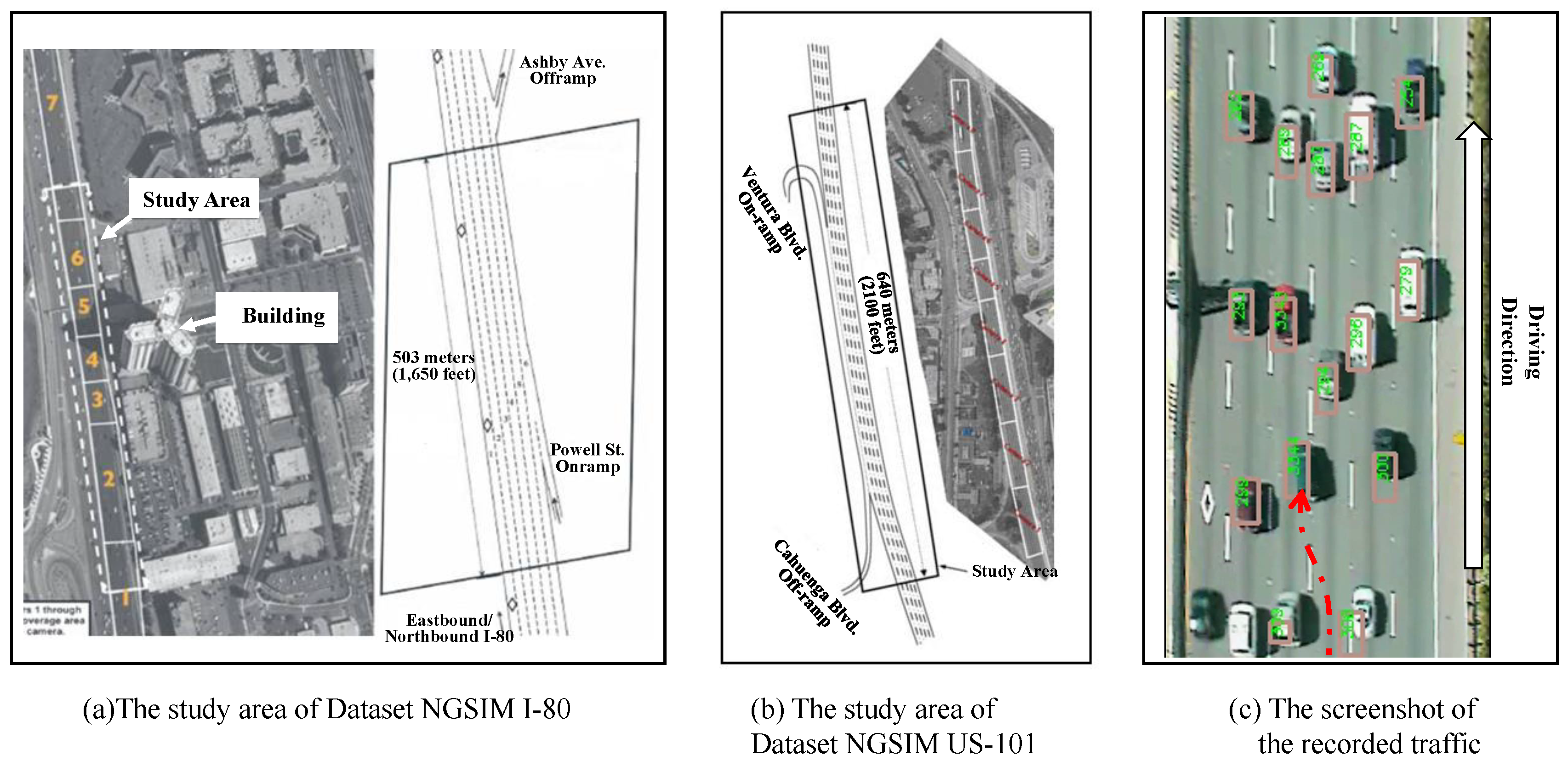
In this section, the detail of our approach executed on real-traffic open datasets is discussed. Moreover, the performance of our prediction method is also evaluated compared with other state-of-the-art methods.

6.1. Datasets

The datasets we used are NGSIM I-80 and NGSIM US-101 from American Federal Highway Administration. They have been widely used for intelligent transportation systems and validation of prediction algorithms (e.g., [40,41]). The two datasets contain six subsets of fifteen-minute collected trajectories (denoting as (I), (II), ⋯, (VI)), which are collected by vision-based highway monitoring systems. The monitoring systems, which can record the real-time traffic as a video (The screenshot of the video can be seen as Figure 5c), are installed above highway near the study area rather than installed in a vehicle. The basic information of each recorded vehicle provided by datasets is obtained from the video analysis. The content of the data file includes the identification number, position, velocity, acceleration, current lane identification, vehicle type of detected vehicles over time at 10 Hz. Next, we will introduce some important quantitative indicators of each dataset individually, followed by the preprocessing of the datasets.

Dataset NGSIM I-80 is collected from the traffic on Interstate 80 in the San Francisco Bay Area, California. The study area is approximately 1650 feet in length with six mainline lanes, including high-occupancy vehicle lanes and an on-ramp, as shown in Figure 5a. The dataset contains trajectories of 5678 individual vehicles, among which 1851 vehicles are changing the lanes.

Dataset NGSIM US-101 is collected from the traffic on Hollywood Freeway, Los Angeles. The study area is approximately 2100 feet in length with five mainline lanes, including high-occupancy vehicle lanes, an on-ramp and an off-ramp, as shown in Figure 5b. The dataset contains trajectories of 4824 individual vehicles, among which 753 vehicles are changing the lanes.

As the positioning data (e.g., positions, velocities, and accelerations) in the NGSIM is obtained from video analysis, they contain a large amount of noise. Therefore, we first use the first-order Savitzky-Golay filtering algorithm [30] to smooth the raw data. Moreover, all ground-truth lane-change maneuvers are extracted if a driving maneuver passes the lane line to its neighboring lane. The lane-change trajectories refer to the ones which cross the lane line and have a fixed distance on both sides of the lane line (0.5 m in this paper).

6.2. Selection for Discretized Parameters

In this section, the selection for discretized parameters (i.e., thresholds for the discretization) is conducted. The threshold parameters contain: (1) the distance threshold $d_{BO}$ of boundaries to the neighboring lane lines, (2) the yaw angle threshold ${\phi }_{YA}$ to the road tangent, (3) the distance threshold of attention areas in neighboring lanes $d_{thre1}$ (for the neighboring vehicles except for the front), (4) the distance threshold of front attention area $d_{thre2}$.

As discussed in Section 5, the optimal threshold parameters in feature extraction can be selected based on the strength of influence of corresponding nodes. Thus, we apply different values for discretization and then generate different learning datasets to obtain probability distributions. In order to ensure the probability distributions are only influenced by the discretized parameters, the learning datasets are chosen from the records of same vehicles. Then, the strengths of the influence of corresponding nodes (i.e., BO, YA, FVRV, LBRV/LARV/RBRV/RARV) with different probability distributions are calculated as (8). As the nodes LBRV/LARV/RBRV/RARV all depend on the threshold $d_{thre1}$, the average strength of the influence of four nodes is calculated.

Table 2. Parameter comparison for boundary distance to the neighbor lanelines $d_{BO}$.

I-80	Threshold for BO (Unit:m)					US-101	Threshold for BO (Unit:m)
	0.3	0.5	0.7	0.9	1.1		0.3	0.5	0.7	0.9	1.1
(I)	0.508	0.554	0.501	0.437	0.350	(IV)	0.330	0.512	0.552	0.503	0.426
(II)	0.495	0.509	0.371	0.294	0.294	(V)	0.289	0.463	0.537	0.512	0.450
(III)	0.468	0.497	0.441	0.373	0.291	(VI)	0.316	0.491	0.575	0.539	0.467

,

Table 3. Parameter comparison for yaw rate to the road tangent ${\phi }_{YA}$.

I-80	Threshold for YA (Unit:degree)					US-101	Threshold for YA (Unit:degree)
	0.5	1	1.5	2	2.5		0.5	1	1.5	2	2.5
(I)	0.674	0.704	0.699	0.675	0.637	(IV)	0.485	0.467	0.403	0.335	0.269
(II)	0.637	0.616	0.599	0.586	0.539	(V)	0.616	0.628	0.595	0.543	0.480
(III)	0.657	0.661	0.649	0.633	0.613	(VI)	0.681	0.675	0.653	0.607	0.539

,

Table 4. Parameter comparison for distance $d_{thre1}$.

I-80	Threshold for Distance ${\mathit{d}}_{\mathit{thre}1}$ (Unit:m)					US-101	Threshold for Distance ${\mathit{d}}_{\mathit{thre}1}$ (Unit:m)
	40	60	80	100	120		120	140	160	180	200
(I)	0.0112	0.0116	0.0117	0.0117	0.0117	(IV)	0.0091	0.0092	0.0091	0.0091	0.0092
(II)	0.0111	0.0114	0.0114	0.0115	0.0114	(V)	0.0084	0.0084	0.0084	0.0084	0.0084
(III)	0.0116	0.0119	0.0119	0.0121	0.0121	(VI)	0.0061	0.0061	0.0062	0.0062	0.0062

and

Table 5. Parameter comparison for distance $d_{thre2}$.

I-80	Threshold for Distance ${\mathit{d}}_{\mathit{thre}2}$ (Unit:m)					US-101	Threshold for Distance ${\mathit{d}}_{\mathit{thre}2}$ (Unit:m)
	10	12	14	16	18		10	12	14	16	18
(I)	0.0170	0.0161	0.0153	0.0145	0.0140	(IV)	0.0130	0.0127	0.0123	0.0119	0.0118
(II)	0.0153	0.0143	0.0135	0.0130	0.0127	(V)	0.0102	0.0099	0.0096	0.0093	0.0092
(III)	0.0149	0.0138	0.0131	0.0127	0.0124	(VI)	0.0079	0.0077	0.0074	0.0071	0.0070

list the calculated strength of influence with different discretized parameters on two datasets. As the strength of the influence shows the predictive capacity, the higher strength of influence is preferred. Consequently, the highest values, which are selected as the optimal parameters, will be used in the following performance experiments. As the tables show, the optimal discretized parameters of these four nodes show high consistency within the two datasets. This indicates that two highways have structural similarities. Moreover, the optimal discretized parameters may vary with different subsets, but the differences are quite small. Surprisingly, in these two datasets, the interaction-aware features show weaker influence compared to other two features (almost an order of magnitude). Table 5 shows that the optimal parameters for the threshold $d_{thre2}$ in both datasets are 10 m. The optimal values are consistent with the dataset description, which indicates a heavy traffic flow in the rushing periods. Table 4 shows that the optimal parameters for the threshold $d_{thre1}$ are 100 m for I-80 and 200 m for US-101, which are much larger than those of $d_{thre2}$. However, the strength of influence only slightly increases with the threshold $d_{thre1}$ from 20 m to 200 m, whose increment is only 0.001. For simplicity, only five thresholds are shown in tables.

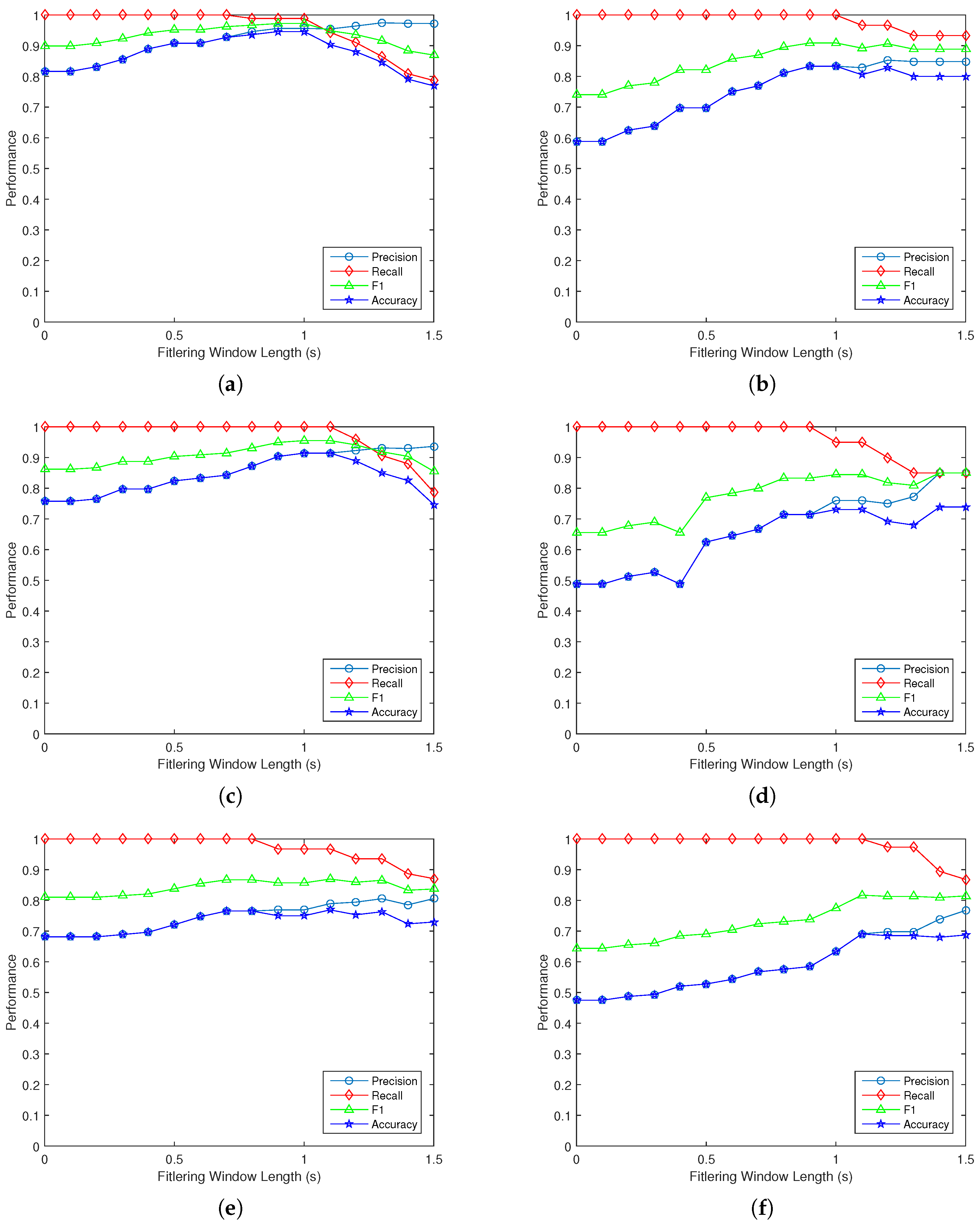
6.3. Performance Metrics and Filtering Window

To comprehensively evaluate the prediction performance, we exploit four quantitative performance metrics, i.e., Precision, Recall, F1 Score, Accuracy. The primary objective of prediction is predicting the lane-change maneuver correctly, which is noted as positive.

(1)

Precision (PRE) is the fraction of correct classification of corresponding lane change out of all events predicted to be positive, i.e.,

$$PRE=\frac{TP}{TP+FP}$$

(9)

where $TP$ means true positive and $FP$ means false positive.

(2)

Recall, also named true positive rate (TPR), is the fraction of correct classification of corresponding lane change out of all true events, i.e.,

$$TPR=\frac{TP}{TP+FN}$$

(10)

where $FN$ means false negative.

(3)

F1 Score is the harmonic mean of the two metrics (precision and recall), i.e.,

$$F1=\frac{2\ast PRE\ast TPR}{PRE+TPR}$$

(11)

(4)

Accuracy (ACC) is the fraction of correctly classified maneuvers out of all predicted maneuvers, i.e.,

$$ACC=\frac{TP+TN}{TP+TN+FP+FN}$$

(12)

where $TN$ means true negative.

To improve the stability of the prediction, we exploit a window filtering algorithm after the Bayesian inference executed. The workflow of window filtering algorithm runs as Figure 6. Each time point, the DBN uses all features to infer the possibility of the maneuvers in two consecutive time slices (i.e., one previous time point and current time point). The maneuver at the current time point with a maximal possibility is chosen as the candidate result. Then, candidate results are put into a fixed-length row (also called filtering window). If all elements in the window are the same lane-change maneuver, the final predicted result will be the same. Otherwise, the final predicted result is lane keeping.

The results for two datasets are shown in Figure 7 and Figure 8, respectively. The figures demonstrate that the time length of the filtering window has important effects on the classification performance. The advantage of a larger filtering window is producing larger PRE and F1 scores in all datasets, which leads to less false alarming. Therefore, the prediction will be more stable. Contrarily, a smaller filtering window produces a larger recall rate in all datasets, which decreases the risk of ignoring the lane change. Consequently, the driving of intelligent vehicles will be more safe-oriented due to being careful to possible lane changes. The trade-off between the precision and recall is common in the field of machine learning. Thus, the time length of the filtering window should be chosen differently according to the traffic scenario. Please note that the number of left-change maneuvers is more than that of right-change maneuvers. Thus, the prediction performance of left-change maneuver is slightly better than that of right-change maneuver.

6.4. Comparison with Other Approaches

To verify the performance of our approach, we compared our approach with other state-of-the-art approaches, which include a model predictive control (MPC)-based approach [43], a Bayesian network-based approach [34], a recurrent neural network (RNN)-based approach [41], a HMM-based approach [44] and a rule-based approach [45].

The settings of comparative experiments are as follows. The discretized parameters for extracting features are selected as

Table 6. Final selected parameters.

Parameter	Dataset I-80	Dataset US-101
boundary distance threshold to the neighbor lane lines (m)	0.5	0.7
yaw rate threshold to the road tangent (deg)	0.5 (II) 1 (I), (III)	0.5 (IV, VI) 1 (V)
the distance threshold of attention areas in neighboring lanes $d_{thre1}$ (m)	100	200
the distance threshold of front attention area $d_{thre2}$ (m)	10	10

. The time length of the filtering window is one second, whose performance has the highest F1 score on average in the previous section. Eighty percent of the lane-change vehicles are randomly chosen from each sub-dataset as the learning set. Then, corresponding networks with learned CPTs are used to predict on ten testing sets. As the experiment based on a Bayesian network approach in [34] is not conducted in the dataset NGSIM, the features for predicting lane-change maneuvers in the original network are reserved with recalculation of the CPTs.

The prediction time is another comparative indicator of different approaches, which shows the capacity to predict lane-change maneuvers in advance. The prediction time is defined as ${\tau }_t=t_e-t_p$, where $t_e$ represents the time point of crossing a lane line, and $t_p$ is the first time point with a lane-change label prediction.

The average metrics of each approach are listed in

Table 7. Performance comparison of different approaches.

Method	Our Approach		MPC-Based [43]		BN Based [34]	RNN Based [41]	HMM Based [44]	Rule Based [45]
Dataset	I-80	US-101	I-80	US-101	Both	Both	Self-collected	I-80 Only
precision	0.73	0.68	0.91	0.89	0.53	[-]	[-]	[-]
recall	0.99	0.89	0.70	0.74	0.72	[-]	[-]	[-]
F1	0.83	0.76	0.78	0.81	0.61	[-]	[-]	[-]
Accuracy	0.72	0.63	0.81	0.82	0.57	0.83–0.89	0.91	0.39
Prediction time	2.39	5.11	4.39	4.73	1.03	[-]	1.5	2

. Among all approaches, the proposed approach retains the highest recall up to 0.94 and the highest average F1 score of 0.795 on average. This shows our approach has a high comprehensive predictive performance. The average prediction time for a lane change after the beginning of a correct prediction is 3.75 s, which is the second highest among all approaches. This demonstrates that the proposed method can provide a long prediction time before the predicting vehicle crosses the lane markers.

It can be seen from the Table 7 that the performance of our approach is much better than the Bayesian network-based approach [34] on all metrics, which implies that the multiple features and dynamic relationship improve the prediction performance. Compared to the rule-based approach which is only conducted in the dataset I-80, our approach is not confined to a single scenario. Though the comprehensive F1 score of our approach is the highest, the accuracy is slightly lower than MPC-based, RNN-based and HMM-based approaches.

It should be pointed out that our approach needs less computational resource compared to the RNN-based approach in the parameter learning process. As the learning process of our DBN uses the maximum likelihood estimation method to estimate parameters as (2), the result can be calculated easily by traversing all instances in the dataset. Thus, the complexity of parameter learning in our approach is $O\left(M\right)$, where M is the number of instances in the dataset. The learning complexity of the RNN, which traditionally uses stochastic gradient descent optimization technique, is $O\left(n^{2}hM\right)$, where n is the number of the nodes, and h is the length of epoch [46].

6.5. Limitation of the Results

Though the performance of maneuver prediction is greatly improved on large-scale and publicly available real-traffic datasets, the following limitation may still exist. (1) The datasets are not collected from the perspective of intelligent vehicles, so final onboard predictions deserve further verification. (2) This paper does not consider the driving behavior which violates traffic rules or out of control driving.

7. Conclusions and Future Work

This paper proposes a maneuver-prediction approach based on the DBN with multi-dimensional predictive features. The experiment is conducted on the publicly available datasets. The results show that the performance of maneuver prediction is greatly improved using our approach, which can recognize the lane-change maneuvers with an F1 of $80\%$ and a prediction time of 3.75 s.

To accurately predict the motion of surrounding vehicles, future work includes predicting long-term trajectories based on the predicted maneuvers, which will take velocity prediction into account. Moreover, a real-time implementation of our approach will be verified in real-world traffic scenarios.

References

1. Jalal, A.; Sarif, N.; Kim, J.T.; Kim, T.S. Human activity recognition via recognized body parts of human depth silhouettes for residents monitoring services at smart home. Indoor Built Environ. 2013, 22, 271–279. [Google Scholar] [CrossRef]
2. Jalal, A.; Rasheed, Y.A. Collaboration achievement along with performance maintenance in video streaming. In Proceedings of the IEEE Conference on Interactive Computer Aided Learning, Villach, Austria, 16–19 October 2007; Volume 2628, p. 18. [Google Scholar]
3. Jalal, A.; Kim, J.T.; Kim, T.S. Human activity recognition using the labeled depth body parts information of depth silhouettes. In Proceedings of the 6th International Symposium on Sustainable Healthy Buildings, Seoul, Korea, 10 February 2012; Volume 27. [Google Scholar]
4. Jalal, A.; Kim, J.T.; Kim, T.S. Development of a life logging system via depth imaging-based human activity recognition for smart homes. In Proceedings of the 6th International Symposium on Sustainable Healthy Buildings, Seoul, Korea, 10 February 2012; Volume 19. [Google Scholar]
5. Jalal, A.; Kim, Y.; Kim, D. Ridge body parts features for human pose estimation and recognition from RGB-D video data. In Proceedings of the International Conference on Computing, Communication and Networking Technologies (ICCCNT), Hefei, China, 11–13 July 2014; pp. 1–6. [Google Scholar]
6. Kamal, S.; Jalal, A.; Kim, D. Depth images-based human detection, tracking and activity recognition using spatiotemporal features and modified HMM. J. Electr. Eng. Technol. 2016, 11, 1921–1926. [Google Scholar] [CrossRef]
7. Liebner, M.; Ruhhammer, C.; Klanner, F.; Stiller, C. Generic driver intent inference based on parametric models. In Proceedings of the IEEE International Conference on Intelligent Transportation Systems, The Hague, The Netherlands, 6–9 October 2013; Volume 5, pp. 268–275. [Google Scholar]
8. Xie, G.; Zhang, X.; Gao, H.; Qian, L.; Wang, J.; Ozguner, U. Situational Assessments Based on Uncertainty-Risk Awareness in Complex Traffic Scenarios. Sustainability 2017, 9, 1582. [Google Scholar] [CrossRef]
9. Lefèvre, S.; Vasquez, D.; Laugier, C. A survey on motion prediction and risk assessment for intelligent vehicles. ROBOMECH J. 2014, 1, 1. [Google Scholar] [CrossRef]
10. Jalal, A.; Kim, S. Global security using human face understanding under vision ubiquitous architecture system. World Acad. Sci. Eng. Technol. 2006, 13, 7–11. [Google Scholar]
11. Farooq, A.; Jalal, A.; Kamal, S. Dense RGB-D map-based human tracking and activity recognition using skin joints features and self-organizing map. KSII Trans. Internet Inf. Syst. 2015, 9, 1856–1869. [Google Scholar]
12. Kamal, S.; Jalal, A. A hybrid feature extraction approach for human detection, tracking and activity recognition using depth sensors. Arab. J. Sci. Eng. 2016, 41, 1043–1051. [Google Scholar] [CrossRef]
13. Xu, W.; Pan, J.; Wei, J.; Dolan, J.M. Motion Planning under Uncertainty for On-Road Autonomous Driving. In Proceedings of the 2014 IEEE International Conference on Robotics & Automation (ICRA), Hong Kong, China, 31 May–7 June 2014; pp. 2507–2512. [Google Scholar]
14. Althoff, M.; Mergel, A. Comparison of Markov chain abstraction and Monte Carlo simulation for the safety assessment of autonomous cars. IEEE Trans. Intell. Transp. Syst. 2011, 12, 1237–1247. [Google Scholar] [CrossRef]
15. Liebner, M.; Baumann, M.; Klanner, F.; Stiller, C. Driver intent inference at urban intersections using the intelligent driver model. IEEE Intell. Veh. Symp. Proc. 2012, 1162–1167. [Google Scholar] [CrossRef]
16. Zhao, H.; Wang, C.; Lin, Y.; Guillemard, F.; Geronimi, S.; Aioun, F. On-Road Vehicle Trajectory Collection and Scene-Based Lane Change Analysis: Part II. IEEE Trans. Intell. Transp. Syst. 2017, 18, 206–220. [Google Scholar] [CrossRef]
17. Althoff, M.; Magdici, S. Set-Based Prediction of Traffic Participants on Arbitrary Road Networks. IEEE Trans. Intell. Veh. 2016, 1, 187–202. [Google Scholar] [CrossRef]
18. Koschi, M.; Althoff, M. SPOT: A tool for set-based prediction of traffic participants. IEEE Intell. Veh. Symp. Proc. 2017, 1686–1693. [Google Scholar] [CrossRef] [Green Version]
19. Schlechtriemen, J.; Wedel, A.; Hillenbrand, J.; Breuel, G.; Kuhnert, K.D. A Lane Change Detection Approach using Feature Ranking with Maximized Predictive Power. In Proceedings of the 2014 IEEE Intelligent Vehicles Symposium (IV), Dearborn, MI, USA, 8–11 June 2014; pp. 108–114. [Google Scholar] [CrossRef]
20. Geng, X.; Liang, H.; Yu, B.; Zhao, P.; He, L.; Huang, R. A Scenario-Adaptive Driving Behavior Prediction Approach to Urban Autonomous Driving. Appl. Sci. 2017, 7, 426. [Google Scholar] [CrossRef]
21. Hu, M.; Liao, Y.; Wang, W.; Li, G.; Cheng, B.; Chen, F. Decision tree-based maneuver prediction for driver rear-end risk-avoidance behaviors in cut-in scenarios. J. Adv. Transp. 2017, 2017. [Google Scholar] [CrossRef]
22. Jo, K.; Lee, M.; Member, S.; Kim, J. Tracking and Behavior Reasoning of Moving Vehicles Based on Roadway Geometry Constraints. IEEE Trans. Intell. Transp. Syst. 2017, 18, 460–476. [Google Scholar] [CrossRef]
23. Xie, G.; Gao, H.; Qian, L.; Huang, B.; Li, K.; Wang, J. Vehicle Trajectory Prediction by Integrating Physics- and Maneuver-based Approaches Using Interactive Multiple Models. IEEE Trans. Ind. Electron. 2017, 65, 5999–6008. [Google Scholar] [CrossRef]
24. Huang, R.; Liang, H.; Zhao, P.; Yu, B.; Geng, X. Intent-Estimation- and Motion-Model-Based Collision Avoidance Method for Autonomous Vehicles in Urban Environments. Appl. Sci. 2017, 7, 457. [Google Scholar] [CrossRef]
25. Xie, G.; Gao, H.; Huang, B.; Qian, L.; Wang, J. A Driving Behavior Awareness Model based on a Dynamic Bayesian Network and Distributed Genetic Algorithm. Int. J. Comput. Intell. Syst. 2018, 11, 469–482. [Google Scholar] [CrossRef]
26. Jalal, A.; Kim, Y.H.; Kim, Y.J.; Kamal, S.; Kim, D. Robust human activity recognition from depth video using spatiotemporal multi-fused features. Pattern Recognit. 2017, 61, 295–308. [Google Scholar] [CrossRef]
27. Lee, D.; Kwon, Y.P.; Mcmains, S.; Hedrick, J.K. Convolution neural network-based lane change intention prediction of surrounding vehicles for ACC. In Proceedings of the IEEE Conference on Intelligent Transportation Systems, Proceedings, ITSC, Yokohama, Japan, 16–19 October 2017; pp. 1–6. [Google Scholar] [CrossRef]
28. Phillips, D.J.; Wheeler, T.A.; Kochenderfer, M.J. Generalizable intention prediction of human drivers at intersections. IEEE Intell. Veh. Symp. Proc. 2017, 1665–1670. [Google Scholar] [CrossRef]
29. Yu, H.; Wu, Z.; Wang, S.; Wang, Y.; Ma, X. Spatiotemporal recurrent convolutional networks for traffic prediction in transportation networks. Sensors 2017, 17, 1501. [Google Scholar] [CrossRef] [PubMed]
30. Altché, F.; de La Fortelle, A. An LSTM Network for Highway Trajectory Prediction. In Proceedings of the IEEE Conference on Intelligent Transportation Systems, Proceedings, ITSC, Yokohama, Japan, 16–19 October 2017. [Google Scholar] [CrossRef]
31. Deo, N.; Rangesh, A.; Trivedi, M.M. How would surround vehicles move? A unified uramework for maneuver classification and motion prediction. IEEE Trans. Intell. Veh. 2018, 3, 129–140. [Google Scholar] [CrossRef]
32. Kasper, D.; Weidl, G.; Dang, T.; Breuel, G.; Tamke, A.; Rosenstiel, W. Object-oriented Bayesian networks for detection of lane change maneuvers. Intell. Transp. Syst. Mag. 2012, 4, 673–678. [Google Scholar] [CrossRef]
33. Gindele, T.; Brechtel, S.; Dillmann, R. Learning driver behavior models from traffic observations for decision making and planning. IEEE Intell. Transp. Syst. Mag. 2015, 7, 69–79. [Google Scholar] [CrossRef]
34. Schreier, M.; Willert, V.; Adamy, J. An Integrated Approach to Maneuver-Based Trajectory Prediction and Criticality Assessment in Arbitrary Road Environments. IEEE Trans. Intell. Transp. Syst. 2016, 17, 2751–2766. [Google Scholar] [CrossRef]
35. Bahram, M.; Hubmann, C.; Lawitzky, A.; Aeberhard, M.; Wollherr, D. A Combined Model- and Learning-Based Framework for Interaction-Aware Maneuver Prediction. IEEE Trans. Intell. Transp. Syst. 2016, 17, 1538–1550. [Google Scholar] [CrossRef]
36. Li, J.; Li, X.; Jiang, B.; Zhu, Q. A maneuver-prediction method based on dynamic bayesian network in highway scenarios. In Proceedings of the 2018 Chinese Control And Decision Conference (CCDC), Shenyang, China, 9–11 June 2018; pp. 3392–3397. [Google Scholar]
37. Agamennoni, G.; Nieto, J.I.; Nebot, E.M. Estimation of multivehicle dynamics by considering contextual information. IEEE Trans. Robot. 2012, 28, 855–870. [Google Scholar] [CrossRef]
38. Koller, D.; Friedman, N.; Bach, F. Probabilistic Graphical Models: Principles and Techniques; MIT Press: Cambridge, MA, USA, 2009. [Google Scholar]
39. Koiter, J.R. Visualizing Inference in Bayesian Networks. Master’s Thesis, Delft University of Technology, Delft, The Netherlands, 16 June 2006. [Google Scholar]
40. Deo, N.; Trivedi, M.M. Convolutional Social Pooling for Vehicle Trajectory Prediction. In Proceedings of the 2018 IEEE/CVF Conference on Computer Vision and Pattern Recognition Workshops (CVPRW), Salt Lake City, UT, USA, 18–22 June 2018. [Google Scholar] [CrossRef]
41. Scheel, O.; Schwarz, L.; Navab, N.; Tombari, F. Situation Assessment for Planning Lane Changes: Combining Recurrent Models and Prediction. In Proceedings of the IEEE International Conference on Robotics and Automation (ICRA), Brisbane, Australia, 21–26 May 2018; p. 7. [Google Scholar]
42. U.S. Department of Transportation. NGSIM—Next Generation Simulation. 2007. Available online: https://ops.fhwa.dot.gov/trafficanalysistools/ngsim.htm (accessed on 22 December 2018).
43. Zhang, Y.; Lin, Q.; Wang, J.; Verwer, S.; Dolan, J.M. Lane-change Intention Estimation for Car-following Control in Autonomous Driving. IEEE Trans. Intell. Veh. 2018, 3, 276–286. [Google Scholar] [CrossRef]
44. Lee, D.; Hansen, A.; Karl Hedrick, J. Probabilistic inference of traffic participants lane change intention for enhancing adaptive cruise control. In Proceedings of the 2017 IEEE Intelligent Vehicles Symposium (IV), Los Angeles, CA, USA, 11–14 June 2017; pp. 855–860. [Google Scholar] [CrossRef]
45. Nilsson, J.; Fredriksson, J.; Coelingh, E. Rule-Based Highway Maneuver Intention Recognition. In Proceedings of the IEEE Conference on Intelligent Transportation Systems, Proceedings, ITSC, Las Palmas, Spain, 15–18 September 2015; pp. 950–955. [Google Scholar] [CrossRef]
46. Sak, H.; Senior, A.; Beaufays, F. Long short-term memory recurrent neural network architectures for large scale acoustic modeling. In Proceedings of the Fifteenth Annual Conference of the International Speech Communication Association, Singapore, 14–18 September 2014. [Google Scholar]
Figure 1. Framework of proposed maneuver-prediction approach.
Electronics 08 00040 g001
Figure 2. Structure of our dynamic Bayesian network for lane-change maneuver prediction.
Electronics 08 00040 g002
Figure 3. The attention area is divided into five sections by the distance thresholds.
Electronics 08 00040 g003
Figure 4. Description of key threshold parameters of the physical-based features: YA and BO.
Electronics 08 00040 g004
Figure 5. Overview of traffic environments on two datasets [42].
Electronics 08 00040 g005
Figure 6. The workflow of window filtering algorithm.
Electronics 08 00040 g006
Figure 7. The impact of the time length of the filtering window on prediction performance in Dataset I-80. The left column shows the prediction performance of left lane changes, and the right column shows that of right lane changes. (a) Performance of left lane change in Dataset (I); (b) Performance of right lane change in Dataset (I); (c) Performance of left lane change in Dataset (II); (d) Performance of right lane change in Dataset (II); (e) Performance of left lane change in Dataset (III); (f) Performance of right lane change in Dataset (III).
Electronics 08 00040 g007
Figure 8. The impact of the time length of the filtering window on prediction performance in Dataset US-101. The left column shows the prediction performance of left lane changes, and the right column shows that of right lane changes. (a) Performance of left lane change in Dataset (IV); (b) Performance of right lane change in Dataset (IV); (c) Performance of left lane change in Dataset (V); (d) Performance of right lane change in Dataset (V); (e) Performance of left lane change in Dataset (VI); (f) Performance of right lane change in Dataset (VI).
Electronics 08 00040 g008