On the Analysis of the Influence of the Evaluation Metric in Community Detection over Social Networks

Abstract

Community detection in social networks is becoming one of the key tasks in social network analysis, since it helps with analyzing groups of users with similar interests. As a consequence, it is possible to detect radicalism or even reduce the size of the data to be analyzed, among other applications. This paper presents a metaheuristic approach based on Greedy Randomized Adaptive Search Procedure (GRASP) methodology for detecting communities in social networks. The community detection problem is modeled as an optimization problem, where the objective function to be optimized is the modularity of the network, a well-known metric in this scientific field. The results obtained outperform classical methods of community detection over a set of real-life instances with respect to the quality of the communities detected.

1. Introduction

The evolution of social networks in the last few decades has aroused the interest of scientists from different and diverse areas, from psychology to computer sciences. Millions of people constantly share all their personal and professional information in several social networks [1]. Furthermore, social networks have become one of the most used information sources, mainly due to their ability to provide the user with real-time content. Social networks are not only a new way of communication, but also a powerful tool that can be used to gather information related to relevant questions. For instance, which is the favourite political party for the next elections?, what are the most commented on movies in the last year?, which is the best rated restaurant in a certain area?, etc.

Extracting relevant information from social networks is a matter of interest mainly due to the huge amount of potential data available. However, traditional network analysis techniques are becoming obsolete because of the exponential growth of the social networks, in terms of the number of active users.

The analysis of social networks has become one of the most popular and challenging tasks in data science [2]. One of the most tackled problems in social networks is the analysis of the relevance of the users in a given social network [3]. The relevance of a user is commonly related to the number of followers or friends that the user has in a certain social network. However, this concept can be extended since a user may be relevant not only if he/she is connected with a large number of users, but also with users that are relevant too. Several metrics have been proposed for analyzing the relevance of a user in a social network, with PageRank emerging as one of the most used [4]. Furthermore, it is interesting to know in advance which users will be the most relevant ones before they become influential [5]. Finally, in the field of marketing analysis, there is special interest in generating the profile of a user given a set of tweets written by that user [6].

Evaluating the relevance of a user has evolved into a more complex problem that consists of detecting specific users (often named influencers) with certain personal attributes that can be personal (credibility or enthusiasm) or related to their social networks (connectivity or centrality). These attributes allow them to influence a large number of users either directly or indirectly [7].

Another important problem regarding the influence of people in other users is the analysis of sentiments in social networks. It is focused on finding out what people think about a certain topic by analyzing the information they post in social networks. We refer the reader to [8] to find a complete survey on sentiment analysis techniques.

The previously described problems deal with only individual users. Nevertheless, some problems also exist related to the structure of the network, devoted to finding specific attributes and properties that can help to infer additional information of the whole social network. In this context, community detection emerges as one of the most studied problems.

Most of the social networks present a common feature named community structure [9]. Networks with this property have the capacity to be divided into groups in such a way that the connections among users in the same group are dense, while connections among users in different groups are sparse. Connections among users can represent different features depending on the social network and the user profile, i.e., from professional relationships to friendships or hobbies in common. Community detection tasks are devoted to finding and analyzing these groups in order to better understand and visualize the structure of network and the relationships among their users.

Performing community detection algorithms over current social networks requires a huge computational effort mainly due to their continuous growth. Furthermore, since these networks are constantly changing (new friendships, mentions to users, viral information, etc.), it is interesting to perform the community detection in the shortest possible computing time, producing real-time information. These features make traditional exact methods not suitable for the current size of social networks, requiring heuristic algorithms in order to accelerate the process without losing quality. Recent works have tackled the community detection problem from a non-exact perspective in order to generate high quality solutions in short computing time [10]. Several studies are devoted to reducing the computational effort for detecting communities in social networks [11,12]. When comparing traditional algorithms over modern large social networks, it can be seen that some of the algorithms require more than 40,000 s for networks with approximately 10,000 nodes, and they are not able to provide a solution after 24 h computing for networks with more than 50,000 nodes.

The growth of social networks complicates their representation and understanding. The communities of a social network usually summarize the whole network but reduce its size and, therefore, makes it easier to analyze. In addition, detecting communities in social networks has several practical applications. Recommendation systems leverage the data of similar users in order to suggest content that can be interesting for them. In order to find similar users in a network, we can simply perform a community detection over the network [13], improving the results of the recommendation system. Communities in social networks also identify people with similar interests, allowing us to evaluate the popularity of a political party [14], or even to detect radicalism in social networks [15].

Although several community detection algorithms exist that have been proposed with the aim of identifying similar users in networks, most of the available algorithms have been designed for optimizing a specific objective function, it being hard to be adapted to a different one (see Section 3 for a detailed description of the considered algorithms). However, the continuous evolution of this area results in a continuous proposal of new metrics that better evaluates the community structure of a given network. This work presents an efficient and versatile algorithm that can be easily adapted to different optimization metrics. To the best of our knowledge, this is the first algorithm based on classical metaheuristics for detecting communities in social networks. The success of this proposal opens a new research line for modeling social network problems as optimization problems, with the aim of applying metaheuristics for solving them.

The main contributions of this work are itemized as follows:

• A new solution representation for the community detection problem is presented.
• A new constructive procedure for generating partitions based on the Greedy Randomized Adaptive Search Procedure (GRASP) is introduced.
• The local search proposed is able to handle not only the change of community of certain nodes, but also the creation and elimination of communities, increasing the portion of search space explored.
• A classical metaheuristic algorithm, GRASP, is adapted to be competitive in social network analysis.
• The proposed algorithm is highly scalable, being easily adapted to be executed in distributed systems.
• A thorough comparison with the most used methods in community detection is provided, analyzing the advantages and disadvantages of each one of them.
• A comparison between two of the most extended metrics is presented, one of them for optimization and the other for evaluation. Furthermore, the evaluation of the metric used for optimization is also performed, with the aim of testing its suitability for the networks considered.

The remainder of the paper is structured as follows: Section 2 formally defines the problem considered as well as the metrics proposed for the evaluation of solutions; Section 3 presents a thorough description of the classical algorithms proposed for detecting communities in social networks; Section 4 presents the new procedure proposed for detecting communities; Section 5 introduces the computational experiments performed to test the quality of the proposal; and finally Section 6 draws some conclusions on the research.

2. Problem Statement

A social network is represented as a graph $G=V,E$, where the set of vertices V, with $\left|V\right|=n$, represents the users of the network and the set of edges E, with $\left|E\right|=m$, represents relations between users belonging to the network. An edge $(v_1,v_2)\in E$, with $v_1,v_2\in V$ can represent different types of relations depending on the social network under consideration. For example, on Twitter, a relation represents that a user follows/is followed by another user, or if there has been some interaction (comment, like, share, etc.) between users, while, on LinkedIn, it represents a professional relationship.

This work is focused on the Community Detection Problem (CDP), which involves grouping users of a social network into communities. A desirable community in a social network is densely connected to the nodes in the same community and sparsely connected (or even unconnected) to nodes in other communities. Therefore, the main objective is to obtain groups or communities of users that are similar and, at the same time, different to the users in other communities with respect to a certain criterion.

A solution for the CDP is represented by a set of decision variables S, with $\left|S\right|=n$, where $S_v=j$ indicates that vertex v is assigned to community j in solution S. Therefore, the community for each vertex $v\in V$ is represented by the corresponding decision variable $S_v$. It is worth mentioning that the number of communities is not predefined in advance. Therefore, a solution where all users are assigned to the same community is feasible. Similarly, a solution where each user is assigned to a different community is also valid.

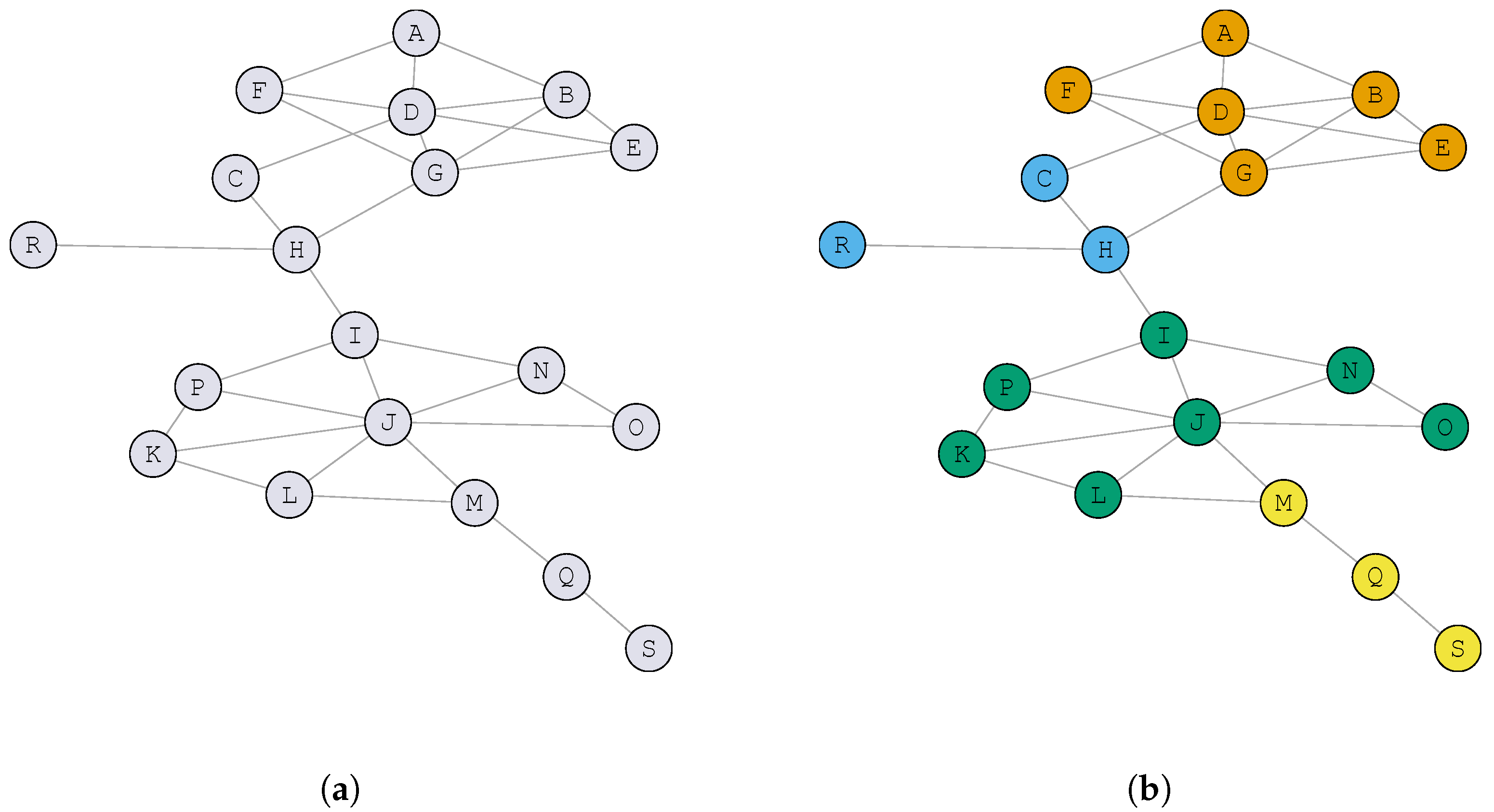
Figure 1a shows an example graph with 19 vertices and 31 edges derived from a social network. In this example, an edge represents a friendship relationship between two users; for instance, users A and B are friends, while users A and C are not friends, but they have a friend in common, which is vertex D.

Figure 1b shows a possible solution S for the community detection problem, where each community is represented with a different color. Notice that, in this example, the number of communities is 4. For the sake of completeness, we report in

Table 1. Community assigned to each vertex in the solution depicted in Figure 1b.

A	B	C	D	E	F	G	H	I	J	K	L	M	N	O	P	Q	R	S
1	1	2	1	1	1	1	2	3	3	3	3	4	3	3	3	4	2	4

the community to which each vertex has been assigned. For example, vertex A belongs to community 1 ($S_A=1$), vertex C to community 2 ($S_C=2$), and so on).

The CDP then consists in finding a solution $S^{\star }$ that maximizes a certain objective function value, denoted as f. In mathematical terms,

$$S^{\star }\leftarrow \underset{S\in \mathbb{S}}{arg\; max}f(S),$$

where $\mathbb{S}$ is the set of all possible solutions for a given social network.

There exists a large variety of quality metrics that can be used as objective functions for finding high quality solutions. Most of the metrics are focused on maximizing the density of intra-community edges (those connecting vertices of the same community) while minimizing inter-community edges (those connecting vertices in different communities).

Notice that the metric considered for optimization is not required from the ground truth since we are dealing with an unsupervised clustering problem [16]. However, some metrics used for evaluating the quality of an algorithm assume that the optimal partition (ground truth) is known beforehand, considering that an algorithm is better if it minimizes the distance from the generated partition to the optimal one. One example of such a metric is the Omega-Index (see [10] for further details). In this work, we consider an alternative approach where the optimal partition is not known.

In this research, we evaluate two metrics that have traditionally been used for optimizing the quality of a solution for the CDP: conductance and modularity [17]. The conductance metric is normalized in the range 0–1, while modularity can take on negative values, ranging from −1/2 to 1. For both metrics, the largest value indicates the value of the optimal partition, while random assignment of users to communities is expected to produce values close to the smallest value. Notice that, in some cases, it is not possible to reach the optimal score due to the internal structure of the network.

The first metric considered in this paper is known as conductance [18]. Given a network G, a solution $S=\{S_1,S_2,\dots ,S_n\}$, and a specific community k, its conductance, $\mathit{Cn}(k,S,G)$, is defined as the number of edges that connect vertices of different communities divided by the minimum between the number of edges with, at least, an endpoint in the community and the number of edges without an endpoint in the community. More formally,

$$\begin{array}{c}\mathit{Cn}(k,S,G)={\displaystyle \frac{|(v,u)\in E:S_v=k\wedge S_u\ne k|}{min\{|(v,u)\in E:S_v=k\vee S_u=k|,|(v,u)\in E:S_v\ne k\wedge S_u\ne k|\}}}.\end{array}$$

Then, the conductance of a complete solution $\mathit{Cn}(S,G)$ is evaluated as the average conductance for all the communities in the graph. In mathematical terms,

$$\begin{array}{c}\mathit{Cn}(S,G)=\sum _{k=1}^{k_{max}}Cn(k,S,G),\end{array}$$

where $k_{max}$ is the number of communities in the incumbent solution S, i.e., $k_{max}=max\{S_1,S_2,\dots ,S_n\}$.

Let us illustrate the computation of this metric with the example depicted in Figure 1b. The conductance of community 2 is evaluated as follows:

$$\begin{array}{cc}\hfill \mathit{Cn}(k,S,G)& ={\displaystyle \frac{|(\mathtt{C},\mathtt{D}),(\mathtt{H},\mathtt{G}),(\mathtt{H},\mathtt{I})|}{min\{|(\mathtt{C},\mathtt{D}),(\mathtt{C},\mathtt{H}),(\mathtt{H},\mathtt{G}),(\mathtt{H},\mathtt{I}),(\mathtt{R},\mathtt{H})|,|E(\mathtt{C},\mathtt{D}),(\mathtt{C},\mathtt{H}),(\mathtt{H},\mathtt{G}),(\mathtt{H},\mathtt{I}),(\mathtt{R},\mathtt{H})|\}}}\hfill \\ & ={\displaystyle \frac{3}{min\{5,26\}}}={\displaystyle \frac{3}{5}}=0.6.\hfill \end{array}$$

Similarly, the conductance of the remaining communities (1, 3, and 4) are $\mathit{Cn}(1,S,G)=0.15$, $\mathit{Cn}(3,S,G)=0.21$, and $\mathit{Cn}(4,S,G)=0.5$, respectively. Therefore, $\mathit{Cn}(S,G)=0.22$.

In order to have a direct comparison with other metrics, it is usually reported the opposite of the conductance evaluated as $\overline{\mathit{Cn}}(G)=1-\mathit{Cn}(G)$. In the aforementioned example, this value is then $\overline{\mathit{Cn}}(G)=0.78$. Then, the objective is to maximize this value to produce high quality solutions.

The second metric is the modularity [19] that evaluates, for each edge connecting vertices in the same community, the probability of the existence of that edge in a random graph. The modularity of a community k over a solution S for a network G is defined as follows:

$$\begin{array}{cc}\hfill \mathit{Md}(k,S,G)& =(e_{jj}-a_j^2),\hfill \\ \hfill e_{kk}& ={\displaystyle \frac{|\{(v,u)\in E:S_v=S_u=k\}|}{\left|E\right|}},\hfill \\ \hfill a_k& ={\displaystyle \frac{|\{(v,u)\in E:S_v=k\}|}{\left|E\right|}},\hfill \end{array}$$

where $k_{\mathit{max}}$ is the number of communities in the solution, $e_{kk}$ is the percentage of intra-community edges (with respect to the whole set of edges) in the community k, and $a_k$ is the percentage of edges with at least one endpoint in k. Then, the modularity of the complete solution S is formally defined as:

$$\begin{array}{c}\hfill \mathit{Md}(S,G)=\sum _{k=1}^{k_{\mathit{max}}}\mathit{Md}(k,S,G).\end{array}$$

Let us illustrate how we can compute this metric for the example depicted in Figure 1b. Specifically, the modularity of community 2 is evaluated as:

$$\begin{array}{cc}\hfill e_{22}& ={\displaystyle \frac{\left|(\mathtt{C},\mathtt{H}),(\mathtt{H},\mathtt{R})\right|}{\left|E\right|}}={\displaystyle \frac{2}{31}},\hfill \\ \hfill a_2& ={\displaystyle \frac{\left|(\mathtt{C},\mathtt{D}),(\mathtt{H},\mathtt{G}),(\mathtt{H},\mathtt{I})\right|}{\left|E\right|}}={\displaystyle \frac{3}{31}},\hfill \\ \hfill \mathit{Md}(2,S,G)& =e_{22}-a_2^2={\displaystyle \frac{2}{31}}-{\left({\displaystyle \frac{3}{31}}\right)}^2=0.06.\hfill \end{array}$$

Similarly, the modularity of the remaining communities (1, 3, and 4) are $\mathit{Md}(1,S,G)=0.35$, $\mathit{Md}(3,S,G)=0.34$, and $\mathit{Md}(4,S,G)=0.06$, respectively. Then, the modularity of the complete solution depicted in Figure 1b is $\mathit{Md}(S,G)=0.75$.

The main disadvantage of modularity metric is its resolution metric. As stated in [20], optimizing modularity may lead the algorithm to miss substructures of the network, thus ignoring the detection of some sub-communities. This behavior does not depend on a particular network structure, but on the ratio between intra-community relations versus the total number of relations in the network.

The majority of the traditional algorithms for community detection considers this metric as the one to be optimized in order to find high-quality partitions in communities, since it does not fall in trivial solutions (i.e., those with a single community for all the network, or those with a different community for each node of the network), being a robust metric to be considered for optimization.

3. Algorithms for Community Detection

Several algorithms have been proposed for detecting communities in social networks (see, for instance, [9,21,22]). Community detection algorithms can be classified into two different classes: agglomerative or divisive. On the one hand, agglomerative methods start from a solution where each vertex is located in a different community and try to optimize a given objective function by joining two or more communities at each step. On the other hand, divisive methods start from a solution with all the vertices located in a single community, and the objective function is optimized by dividing one or more communities in each step.

Most of the algorithms are not exact procedures, since in most of the networks it is not feasible to find the optimal solution in a reasonable time, mainly due to the number of users in the network [19,23]. This section is devoted to describing the most used algorithms in the state of the art for the CDP, in order to have a framework of comparison for the algorithm presented in this work.

3.1. Edge-Betwenness (EB)

The idea of the Edge-Betweenness algorithm [9] relies on identifying those vertices that appear in the majority of the paths in the graph. Specifically, authors define the betweenness of an edge as the number of shortest paths between pairs of vertices that contains the edge under evaluation. Therefore, groups or communities are generated by removing the edge with the largest edge betweenness value in each step. This algorithm has a computational complexity of $O(m^{2}n)$.

3.2. Fast-Greedy (FG)

The Fast-Greedy algorithm [21] is focused on optimizing the modularity of the solutions generated. This agglomerative method starts from a solution where each vertex is located in a different community and iteratively joins the two communities that produce the solution with maximum modularity value. The optimization and data structures presented in the original work reduces the computational complexity of the algorithm to $O(n·m·logn)$.

3.3. Infomap (IM)

The Infomap algorithm [22] proposed a fast stochastic and recursive search method which is based on joining neighbor vertices into the same community. The method starts with each vertex located in a different community. Then, it randomly selects a vertex and assigns it to the community that minimizes the map equation, presented in the original work [22], which is an efficient estimation of the optimality of a certain partition. Then, the method creates a new network where the new vertices are the communities detected until now. The algorithm stops when no changes are produced in the communities.

3.4. Label Propagation (LP)

The Label Propagation algorithm [24] initially assigns a different label to each vertex of the graph. Then, in each iteration, the algorithm modifies the label of each vertex depending on the label assigned to its adjacent vertices. Specifically, a vertex receives the most common label in all its neighbors, stopping when no changes are produced in the labels of the graph. At the end of the process, the label of a vertex identifies the community to which that vertex belongs to. It is worth mentioning that this algorithm does not consider any quality metric, since the optimization is performed with respect to the labels of the neighbors of each vertex. The main advantage of this algorithm is its computational complexity of $O(n+m)$.

3.5. Multi-Level (ML)

The Multi-Level algorithm [11] is designed for detecting communities in large networks focused on optimizing the modularity of the solution. The algorithm consists of two well-differenced phases. The first phase starts by assigning each vertex to a different community. In each step, the method evaluates, for each vertex v, the profit of merging it in the community of each adjacent vertex in terms of modularity. Then, vertex v is inserted in the community that produces the maximum profit, only if the profit is positive, stopping when no improvement can be found. The second phase is based on creating a new network where each node represents a community, where the weights of the edges identifies the sum of the weights of the edges between nodes in the corresponding communities. Then, the first phase is applied again to this new network. The two phases are iteratively applied until no changes are performed in the communities detected. The main advantage of this algorithm relies on the efficient evaluation of the profit in terms of modularity, resulting in a linear complexity when the number of vertices is similar to the number of edges. However, if the graph is fully connected, the algorithm presents a complexity of $O(n^2)$.

3.6. Spinglass (SG)

The Spinglass algorithm [25] is inspired by statistical physics, in particular in the Potts model. The algorithm simulates that each vertex of the graph is a particle that can have any of the spin states. Additionally, the edges represent the interactions between particles, which influence the vertices in changing their spin state or not. Then, the method simulates the model a predefined number of iterations. Finally, the spin state of each particle identifies the community of each vertex. It is a computationally demanding algorithm mainly due to the simulation and it is not deterministic.

3.7. Walktrap (WT)

The Walktrap algorithm [12] relies on the idea that random walks over a graph usually get caught in the most densely connected parts, which are often the communities of the graph. Then, authors define a distance that can be evaluated efficiently. This distance is then used in a hierarchical clustering algorithm that iteratively merges vertices into communities, creating a dendogram of the community structure of the graph. The complexity of the method is $O(mnH)$, H being the height of the dendogram. The worst case corresponds to a dendogram of height n, resulting in a complexity of $O(m{n}^2)$, which corresponds to very dense graphs. However, real-life social networks are usually sparse, and when H is small and the dendogram is balanced, the complexity is reduced to $O(n^{2}logn)$.

3.8. Louvain (CL)

The Louvain algorithm [11] proposed a method divided into two phases: the first phase considers that each node is initially a community in a network. Then, it joins communities looking for the modularity metric optimization, and stops when a local maximum of modularity is reached. In the second phase, the algorithm builds a new graph with the communities obtained from the first phase, restarting with the first phase. According to [11], this method has a complexity of $O(n)$.

3.9. Evaluation of the Previous Methods

This section is devoted to evaluating the results obtained by the previously described methods over an example graph that presents community structure [26] to provide an illustrative example. Figure 2 depicts the graphical results over the community detection in the graph, where each community is represented with a different color.

As can be seen, the results are different for each algorithm. Additionally, 

Table 2. Evaluation of the solution generated by each algorithm over the example graph using the three considered metrics.

Algorithm	Modularity	Conductance	Number of Communities
EB	0.5245	0.5248	6
FG	0.5284	0.5306	6
LP	0.3596	0.4571	4
ML	0.5158	0.5191	6
SG	0.5257	0.5009	7
WT	0.4927	0.5260	6
IM	0.5231	0.4732	8
CL	0.5158	0.5191	6

presents the results obtained by each considered algorithm over the example graph depicted in Figure 2, considering the two metrics described in Section 2 and the number of communities found.

First of all, we will analyze the modularity metric, since it is the most used metric in community detection optimization and, furthermore, it is the metric to be optimized in the current research. The best modularity value is obtained with the Fast-Greedy algorithm (0.5284), closely followed by Spinglass (0.5257), Edge Betweenness (0.5245) and Infomap (0.5231).

Analyzing the conductance value, the three considered algorithms present the same behavior as with modularity: Fast-Greedy is the best approach (0.5306), but now followed by Walktrap (0.5260) and then Edge Betweenness (0.5248). Notice that the differences among algorithms considering conductance are larger.

Finally, analyzing the number of communities detected, five out of the eight algorithms detect six communities, which seem to be the actual number of communities in the social network. The largest number of communities, 8, is found with the Infomap algorithm. These results suggests that artificially increasing the number of communities does not lead to better results.

4. Greedy Randomized Adaptive Search Procedure

Metaheuristics comprehend a set of approximate algorithms designed for solving hard combinatorial optimization problems for which traditional heuristic methods are not effective. These algorithms provide a general framework for creating new hybrid algorithms with concepts derived from artificial intelligence, biological evolution and statistical mechanisms [27].

Greedy Randomized Adaptive Search Procedure (GRASP) is a metaheuristic originally presented in [28] and formally defined in [29]. We refer the reader to [30] for a recent survey on this methodology. This metaheuristic can be divided into two main phases: solution construction and local improvement.

The first phase iteratively adds elements to an initially empty solution until it becomes feasible. The first element is usually selected at random, acting as a seed for the procedure. The algorithm then constructs a candidate list (CL) with all the elements that must be included in the solution. After that, a Restricted Candidate List (RCL) is created with the most promising elements of the CL according to a predefined greedy function. Then, in each iteration, an element is selected at random from the RCL and added to the solution under construction, updating the CL and RCL in each step until reaching a feasible solution.

The construction phase of the GRASP algorithm presents a random part devoted to increasing the diversity of the solutions generated. In particular, in the previous description, the random part relies on the random selection of the next element from the RCL. Therefore, most of the obtained solutions are not local optimum and can be improved by means of a local optimizer. The second phase of the GRASP algorithm is intended to find a local optimum of the solution generated, usually applying a local search method, although it can be replaced with a more complex optimizer, like Tabu Search or Variable Neighborhood Search, for instance [31,32,33].

The algorithm presented in this section is able to optimize any of the metrics defined in Section 1. However, heavily optimizing conductance usually leads to the trivial partition where all the vertices are in the same community. Therefore, the proposed algorithm is focused on optimizing the modularity, which has been traditionally considered as a good optimization metric.

Analyzing the related literature, most of the algorithms are designed for optimizing a specific objective function value. However, the versatility of the proposed algorithm allows it to be easily adapted to optimize either a new or a traditional metric, which converts it into a generic algorithm for finding community structures for any optimization metric.

Furthermore, the algorithm is proposed as a framework for detecting communities. It is easy to replace the constructive method or local search procedure proposed with a different one, or even embed a more complex local optimizer, such as Tabu Search [34], or Variable Neighborhood Search [35], among others.

4.1. Constructive Procedure

The constructive procedure designed for the community detection problem, named GRASPAGG follows an agglomerative approach, where each element is initially located in a different community. Then, GRASPAGG iteratively joins two of the most promising communities with the objective of maximizing the modularity. Algorithm 1 shows the pseudocode of the GRASPAGG constructive method.

Algorithm 1$\mathit{GRASPAGG}(G,\alpha )$.

1: $S_v\leftarrow v\forall v\in V$    2: $\mathit{CL}\leftarrow \{1,2,\dots n\}$    3: while$\mathit{CL}\ne \varnothing$do    4:     $g_{min}\leftarrow {min}_{j\in CL}\mathit{Md}(S,G,j)$    5:     $g_{max}\leftarrow {max}_{j\in CL}\mathit{Md}(S,G,j)$    6:     $\mu \leftarrow g_{min}+\alpha ·(g_{max}-g_{min})$    7:     $\mathit{RCL}\leftarrow \{j\in \mathit{CL}:\mathit{Md}(S,G,j)\ge \mu \}$    8:     $j_1\leftarrow \mathit{Random}(\mathit{RCL})$    9:     $j_2\leftarrow \mathit{IdentifyBestJoin}(S,j_1)$   10:     $S^{\prime }\leftarrow \mathit{Join}(S,j_1,j_2)$   11:     if $f(S^{\prime })>f(S)$ then   12:         $S\leftarrow S^{\prime }$   13:         $\mathit{CL}\leftarrow \mathit{CL}\setminus \{j_2\}$   14:     else   15:         $\mathit{CL}\leftarrow \mathit{CL}\setminus \{j_1\}$   16:     end if   17: end while   18: returnS

The method starts by assigning a different community to each node in the graph G (step 1), creating the CL with every community in the solution S under construction (step 2). In other words, at the beginning of the construction, there will be n nodes assigned to n different communities. Then, the minimum ($g_{min}$) and maximum ($g_{max}$) values for the greedy function under evaluation are calculated (steps 4 and 5). We propose as a greedy function the modularity value of each community j. A threshold $\mu$ is evaluated (step 6) to construct the RCL with the most promising candidates in CL (step 7). The next steps select the two communities that will be joined in the current iteration. The first one, $j_1$, is selected at random from the RCL (step 8). The second community $j_2$ is the one that maximizes the modularity of the resulting solution after joining communities $j_1$ and $j_2$ (step 9). If the method has found an improvement in the modularity after joining both communities, a new iteration is performed, updating the incumbent solution (step 12) and the candidate list (step 13); otherwise, the community $j_1$ is removed from the candidate list since any join involving $j_1$ produces a worse solution. Finally, GRASPAGG stops when it is not possible to join two communities improving the modularity, returning the best solution found.

4.2. Local Optimization

This section presents a local search procedure designed to find a local optimum for every solution constructed in the previous phase. In order to define a local search method, we firstly need to define the neighborhood in which the local optimum will be found. For this problem, we consider all the solutions that can be reached from a given solution S by removing one node from its current community and inserting it in a different one. Specifically, after performing the move $\mathit{Move}(S,v,j)$, the vertex v will be located at community j (i.e., $S_v=j$).The neighborhood $N(S)$ is defined as:

$$\begin{array}{c}N(S)\leftarrow \{\mathit{Move}(S,v,j)\forall v\in S:j\ne S_v\}.\end{array}$$

It is worth mentioning that the number of communities is not a priori defined for the problem. Therefore, if v is the last vertex in the community $j^{\prime }$, then community $j^{\prime }$ will disappear after performing the corresponding move. In the same line, the method also considers creating a new community for vertex v if it improves the modularity. Thus, after performing the local search method, the number of communities may have varied either increasing or decreasing.

The next step for defining the local search method is the selection of the vertex to be moved to another community. For this purpose, we define a heuristic criteria based on the number of intra-community edges of the vertex under evaluation with respect to the total number of edges in the graph. Specifically, the local search method selects the vertex v with the smallest ratio r between number of edges in the same community and the total number of incident edges to v. More formally,

$$\begin{array}{c}r(v,S)\leftarrow {\displaystyle \frac{|(v,u)\in E:S_v=S_u|}{\left|E\right|}}\forall u,w\in V.\end{array}$$

The local search method traverses all the nodes in the solution following an ascending order with respect to the previously defined criterion. Each node is moved from its current community to the one that maximizes the modularity among all the existing communities in the incumbent solution.

The proposed local search procedure follows a first improvement approach. In particular, given a solution S, this strategy scans its neighborhood $N(S)$ in search for the first solution $S^{\prime }\in N(S)$ such that $f(S^{\prime })>f(S)$. The method stops when no improvement is found after exploring the whole neighborhood.

4.3. Complexity Analysis

The complexity analysis of the proposed algorithm can be split into two different stages: constructive and local improvement. Firstly, the complexity of the constructive procedure is analyzed.

The constructive procedure iterates until the candidate list is empty. One candidate is removed in each iteration, either due to the joining of two communities or because the candidate cannot be joined. Following a straightforward implementation, this method requires traversing all the nodes and all the edges, resulting in a complexity of $O(n·m)$. However, we cache the degree of each node and its adjacents in efficient data structures when reading the social network (since the degree of a node will not change during the execution). Therefore, we reduce the complexity of generating the candidate list to $O(n)$. The method then iterates until no improvement in the modularity is found when joining two clusters. In the worst case, it requires performing $n-1$ iterations, resulting in a total complexity of $O(n^2)$. However, we select in each iteration the community with the smallest modularity value, finding improvements in the first iterations. Therefore, the complexity of this stage is $O(logn)$, mainly due to the cost of maintaining the communities sorted by modularity. Finally, the complexity of the complete constructive procedure is $O(nlogn)$.

The second stage corresponds to the local search procedure, where each node is considered to be inserted in each community. Therefore, it presents a complexity of $O(n·k)$, k being the number of communities. However, it is worth mentioning that notation $O()$ refers to the worst case, and it is possible to optimize the search with the aim of avoiding the worst case. In particular, the local search method evaluates each node $v\in S$ following an ascending order (worst nodes first) with respect to the ratio $r(v,S)$ defined in Section 4.2. This ordering is a heuristic that minimizes the number of movements performed before finding an improvement, since it is presumed that nodes with a small ratio value are not located in the best community. Therefore, on average, the algorithm complexity linearly grows with the problem size.

Analyzing the complexity of both stages, the resulting GRASP algorithm presents a global complexity of $O(nlogn)$ plus the complexity of the local search, which is linear (in the average case) with respect to the problem size, resulting in a final complexity of $O(nlogn)$ per iteration.

5. Computational Results

This section is devoted to analyzing the quality of the proposed algorithm when compared with the most popular community detection algorithms presented in Section 3. Since most of the algorithms are focused on optimizing the modularity, the evaluation of the quality must be performed over a different metric. In this work, we consider the conductance with the aim of testing the robustness of the methods when including one additional metric. We also consider the modularity value obtained with each algorithm, although it should not be taken into account in the evaluation of the quality of the community detection. However, we consider that it is interesting to analyze how far an algorithm is able to optimize the detection considering the modularity value. The proposed algorithm has been implemented in Java 8 and the experiments have been conducted in an Intel Core 2 Duo E7300 2.66 GHz with 4 GB RAM.

The instances used for the experiment have been extracted from the Twitter SNAP dataset [36] and from Network repository [37]. Specifically, we have selected 100 instances with vertices ranging from 50 to 400 that represent the ego-network of several Twitter users (data is anonymized in the dataset, and the ego user is not included in it) and other interactions between users from other networks.

The first experiment is devoted to tuning the $\alpha$ parameter of the GRASPAGG procedure. This parameter controls the degree of randomness of the method: on the one hand, $\alpha$ = 0 results in a totally random method, while $\alpha$ = 1 considers a completely greedy method. Therefore, it is interesting to test values distributed in the range 0–1 to analyze whether the best results for the CDP are obtained with a small or large percentage of randomness/greediness in the construction. In this experiment, we have considered $\alpha =\{0.25,0.50,0.75,\mathit{RND}\}$, where RND indicates that a random value of $\alpha$ is selected for each construction. This experiment has been conducted over a subset of 20 representative instances in order to avoid overfitting.

Table 3. Results obtained by the GRASPAGG algorithm considering different values for $\alpha$ parameter.

$\mathit{\alpha }$	Avg. Modularity	#Best
0.25	0.31961	6
0.50	0.32019	5
0.75	0.32063	4
RND	0.32080	9

reports the results obtained with the different values of $\alpha$. Specifically, two statistics are considered: Avg., the average of the best modularity value obtained for each instance, and #Best, the number of times that an algorithm matches that best solution. Notice that conductance is not included in this preliminary experiment since it is performed for tuning the algorithm, and conductance should be used only for evaluating its quality.

Analyzing the results presented in Table 3, we can clearly see that $\alpha =\mathit{RND}$ is able to obtain the largest number of best solutions (9 out of 20). However, the quality of the solutions provided when it does not match the best solution is considerably worse than the other $\alpha$ values. If we now analyze the average modularity value and the number of times that the algorithms reach the best solution, we can conclude that a random value for $\alpha$ in each iteration obtains the best results, closely followed by $\alpha =0.75$. Therefore, the final version of the algorithm is configured with $\alpha =\mathit{RND}$.

Once the best $\alpha$ parameter for the proposed algorithm has been adjusted, it is necessary to compare its performance with the most used community detection algorithms found in the literature. Specifically, we have included in the comparison the algorithms described in Section 3: Edge Betweenness (EB), Fast-Greedy (FG), Label Propagation (LP), Multi-level (ML), Walktrap(WT), InfoMap (IM) and Louvain (CL).

Table 4. Comparison of the considered metrics over all the algorithms presented in Section 3 and the proposed GRASPAGG method.

Algorithm	Modularity		Conductance
	Avg.	#Best	Avg.	#Best
EB	0.20176	0	0.03363	7
FG	0.29441	3	0.44062	17
LP	0.15170	2	0.43734	6
ML	0.28843	2	0.43433	19
WT	0.26663	2	0.25224	7
IM	0.20611	2	0.37829	16
CL	0.31181	33	0.48002	9
GRASPAGG	0.31331	78	0.49483	37

shows the aforementioned comparison.

Firstly, the analysis will be focused on the modularity value. In particular, GRASPAGG is able to obtain a slightly better result than Louvain (0.31331 vs. 0.31181), which is the second best approach. However, regarding the number of best solutions found, we can clearly see the superiority of our proposal, doubling the number of best solutions found with the Louvain method. Then, the next best algorithm is Fast-Greedy, achieving a total of three best solutions found. It is worth mentioning that the remaining algorithms are far from the results with respect to modularity. This can be partially explained since not all the algorithms are focused on optimizing modularity. Therefore, we need to consider an additional metric to have a fair comparison.

The conductance metric should be the one considered for evaluating the performance of each algorithm, since it is an objective metric that has not been used for any of the compared methods. The results show that the trend continues but with more significant differences among methods. Again, the best average conductance value is obtained by GRASPAGG (0.49483), and the second best value is reached with the Louvain method (0.48002). However, the differences between both results are larger, confirming the superiority of our proposal. Additionally, the GRASPAGG method is able to reach 37 out of 100 instances, while Louvain only obtains nine. The third best algorithm is again Fast-Greedy, with a conductance of 0.44062. Notice that, although the conductance of Louvain is better than the one of Fast-Greedy, the latter is able to achieve a larger number of best solutions found (17 vs. 9). The same conclusions can be derived when analyzing Multi-level and Infomap algorithms.

Finally, we have conducted different statistical tests to validate the results reported in Table 4. In particular, we have performed the Friedman non-parametric statistical test with all the individual values obtained in the previous experiment to confirm whether there exist statistically significant differences among the compared algorithms or not. The Friedman test ranks each algorithm according to the conductance value obtained, giving rank 1 to the best algorithm, 2 to the second one, and so on. The larger the differences in the average, the smaller the p-value will be. The average ranks values obtained with this test are GRASPAGG (1.70), CL (2.47), LP (2.73), FG (2.88), ML (3.30), IM (4.12), WT (5.04), and EB (5.74), resulting in a p-value smaller than 0.00001. Additionally, we have performed the Wilcoxon signed rank test for the best two algorithms (i.e., GRASPAGG and CL). The resulting p-value smaller than 0.00001 confirms that there are statistically significant differences between both algorithms, then supporting the quality of the proposed GRASP method.

6. Conclusions

This paper has proposed a new metaheuristic method for community detection in a social network based on Greedy Randomized Adaptive Search Procedure methodology. The problem is addressed by optimizing the modularity metric, which is a robust metric to evaluate the quality of a partition in a social network.

The proposed algorithm is composed of two heuristic strategies. On the one hand, a constructive procedure based on an agglomerative scheme is proposed, which tries to balance the randomness and greediness of the search. On the other hand, an improvement procedure based on a problem-dependent neighborhood definition is presented. The main advantage of this local search is not only to find the best community for each node, but also to create and destroy communities in the incumbent solution.

The experiments firstly select the best value for the algorithm parameters and then compare its results with the most used algorithms for community detection found in the literature. The computational results show how GRASPAGG is able to obtain better results in both metrics than the previous methods. Additionally, the statistical tests performed over the evaluation metric support the quality of the proposed algorithm, emerging as a competitive algorithm for detecting communities in social networks.