SBL-Based Direction Finding Method with Imperfect Array

Abstract

The imperfect array degrades the direction finding performance. In this paper, we investigate the direction finding problem in uniform linear array (ULA) system with unknown mutual coupling effect between antennas. By exploiting the target sparsity in the spatial domain, the sparse Bayesian learning (SBL)-based model is proposed and converts the direction finding problem into a sparse reconstruction problem. In the sparse-based model, the off-grid errors are introduced by discretizing the direction area into grids. Therefore, an off-grid SBL model with mutual coupling vector is proposed to overcome both the mutual coupling and the off-grid effect. With the distribution assumptions of unknown parameters including the noise variance, the off-grid vector, the received signals and the mutual coupling vector, a novel direction finding method based on SBL with unknown mutual coupling effect named DFSMC is proposed, where an expectation-maximum (EM)-based step is adopted by deriving the estimation expressions for all the unknown parameters theoretically. Simulation results show that the proposed DFSMC method can outperform state-of-the-art direction finding methods significantly in the array system with unknown mutual coupling effect.

1. Introduction

In the direction finding problem, the traditional discrete Fourier transform (DFT)-based method can only find one signal in one beam-width, so the resolution of such a method is too low to estimate multiple signals. Therefore, the super-resolution methods have been proposed including multiple signal classification (MUSIC) method [1,2], Root-MUSIC method [3], and the estimating signal parameters via rotational invariance techniques (ESPRIT) method [4]. Additionally, the subspace methods have also been improved to estimate the correlation signals, such as the spatial smoothing MUSIC method [5]. However, the subspace methods only distinguish the noise and signal subspaces and have not exploited additional characteristics of the received signals.

The compressed sensing (CS)-based methods have been proposed to estimate the directions by exploiting the signal sparsity in the spatial domain [6,7,8,9,10,11,12,13,14]. Notably, the sparse Bayesian learning (SBL) and the relevance vector machine (RVM) proposed in [15] can achieve better estimation performance in the CS-based direction finding methods, where the directions are estimated by reconstructing the sparse signals in the spatial domain with the corresponding distribution assumptions of unknown parameters. Consequently, the SBL-based CS method, named CS-SBL, is developed in [16] to reconstruct the sparse signals. However, in the CS-SBL method, the discrete grids are adopted to formulate the CS-based system model, so the estimation performance is limited by the grid size. To further improve the estimation performance, dense grids can be adopted, but it will improve the computational complexity in the sparse reconstruction algorithm.

Additionally, the dense grids improve the correlation between the grids and decrease the performance of sparse reconstruction. The off-grid CS-based methods were proposed [17,18] to overcome the grid problem in the CS-based model, such as the off-grid sparse Bayesian inference (OGSBI) method proposed in [19]. In the off-grid CS-based system model, the ground-truth directions are approximated by the Taylor expansion, so the performance of direction estimation can be improved in the off-grid methods when the same grids are adopted. Moreover, by solving the roots of a specific polynomial in an off-grid model, the Root-SBL method [20] was also proposed to decrease the computational complexity of the SBL-based method. The grid evolution method was proposed in [21] to refine the grids for the SBL-based method, and a dictionary learning algorithm is proposed in [22].

In a practical direction finding problem, the imperfection of the antenna array will decrease the estimation performance, so the mutual coupling effect between antennas cannot be ignored [23,24]. The direction finding methods were proposed in [25,26,27] to decrease the mutual coupling effect. However, in the existing sparse-based methods, the unknown mutual coupling effect is not considered, especially in a scenario with off-grid effect.

In this paper, a symmetric Toeplitz matrix [28,29,30] is used to describe the mutual coupling effect, and a novel direction estimation method is proposed. With both the off-grid and the mutual coupling effect, the direction finding problem is investigated. A novel system model is formulated to describe both the off-grid and the mutual coupling effect. Then, by exploiting the signal sparsity in the spatial domain, a novel direction finding method based on SBL with unknown mutual coupling effect, named DFSMC, is proposed. Additionally, with the distribution assumptions, we theoretically derive the estimation of all unknown parameters using the expectation-maximum (EM)-based method in DFSMC, where the unknown parameters include the mutual coupling vector, the noise variance, the signals, the off-grid vector, et al. Finally, the proposed DFSMC method is compared with the state-of-art methods in the direction finding performance. To summarize, we make the contributions as follows:

• The SBL-based system model with mutual coupling effect: With considering both the off-grid and the unknown mutual coupling problems, a novel system model is formulated and transforms the direction finding problems into a sparse reconstruction problem.
• The DFSM method for direction finding estimation: With the distribution assumptions of all unknown parameters, a novel SBL-based direction finding method with unknown mutual coupling effect, named DFSMC, is proposed. DFSMC method estimates the directions via updating all the unknown parameters alternatively and achieves better estimation performance than the state-of-art methods.
• The theoretical estimation expressions for all unknown parameters: In the proposed DFSMC method, the EM method is adopted to estimate all the unknown parameters including the noise variance, the received signals, the mutual coupling vector, and the off-grid vectors, et al. With the distribution assumptions, we theoretically derive the expressions for all the unknown parameters.

The remainder of this paper is organized as follows. The system model for direction finding with unknown mutual coupling effect is formulated in Section 2. The direction finding method based on SBL is given in Section 3. The simulation results are given in Section 4. Finally, Section 5 concludes the paper.

Notations:${\mathit{I}}_N$ denotes an $N\times N$ identity matrix. $\mathcal{E}\left\{·\right\}$ denotes the expectation operation. $\mathcal{CN}\left(\mathit{a},\mathit{B}\right)$ denotes the complex Gaussian distribution with the mean being $\mathit{a}$ and the covariance matrix being $\mathit{B}$. ${\parallel ·\parallel }_2$, ⊗, $Tr\left\{·\right\}$, ${\left(·\right)}^{\ast }$, ${\left(·\right)}^{\mathrm{T}}$ and ${\left(·\right)}^{\mathrm{H}}$ denote the ${\ell }_2$ norm, the Kronecker product, the trace of a matrix, the conjugate, the matrix transpose and the Hermitian transpose, respectively. $\mathcal{R}\left\{a\right\}$ denotes the real part of complex value a. Additionally, for a vector $\mathit{a}$, ${\left[\mathit{a}\right]}_n$ denotes the n-th entry of $\mathit{a}$, and $diag\left\{\mathit{a}\right\}$ denotes a diagonal matrix with the diagonal entries from $\mathit{a}$. For a matrix $\mathit{A}$, ${\mathit{A}}_{:,n}$ denotes the n-th column of $\mathit{A}$, and $diag\left\{\mathit{A}\right\}$ denotes a vector with the entries from the diagonal entries of $\mathit{A}$.

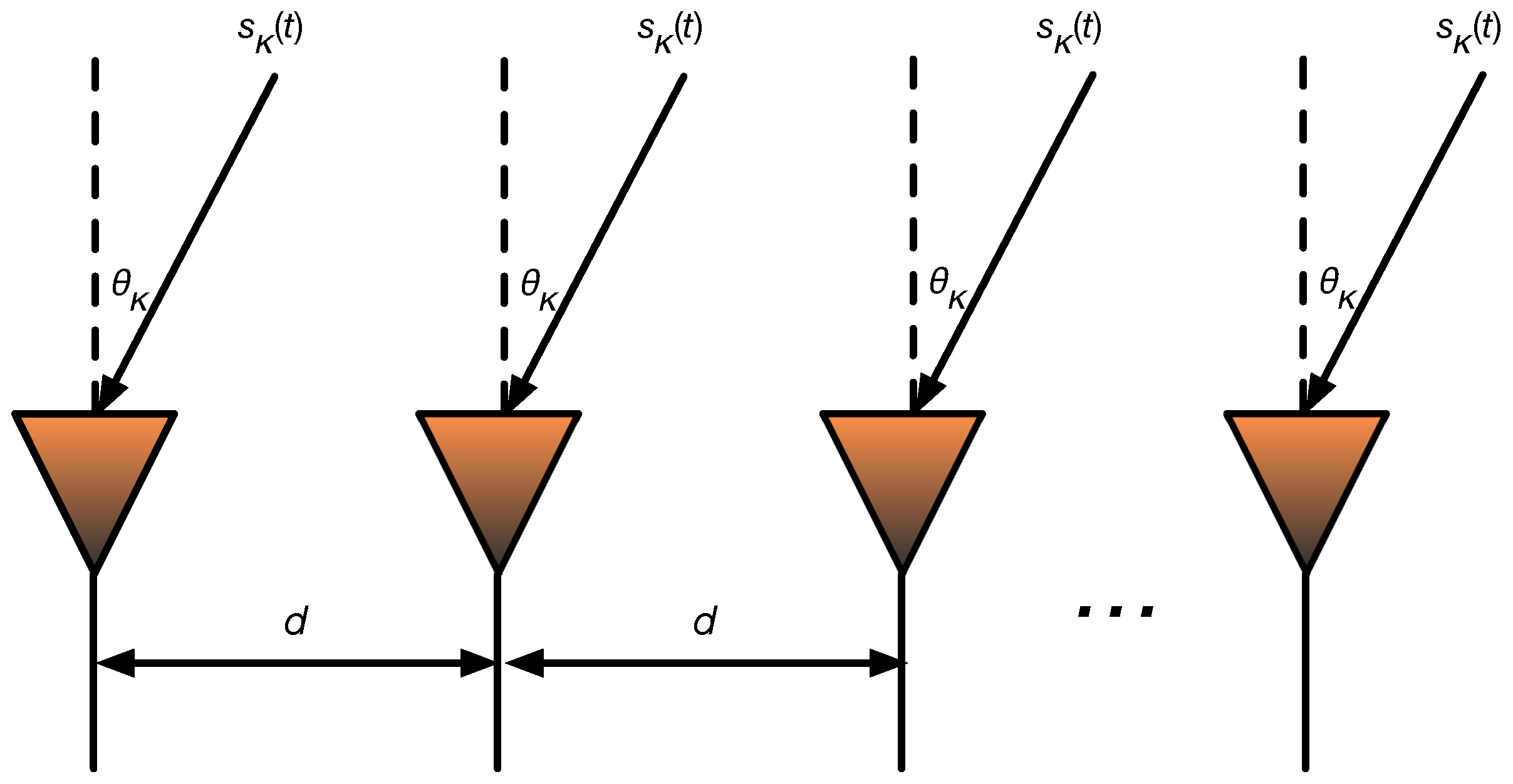
2. ULA System for Direction Finding

We consider the direction finding problem in the uniform linear array (ULA) system, where N antennas are adopted and the inter-antenna element spacing is d. As shown in Figure 1, K unknown signals with different directions (${\theta }_k$, $K=0,1,\dots ,K-1$) are received by the ULA. Thus, the received signals in the N antennas can be expressed as

$$\begin{array}{cc}\hfill \mathit{y}\left(t\right)& ={\displaystyle \sum _{k=0}^{K-1}}\mathit{C}\mathit{a}\left({\theta }_k\right)s_k\left(t\right)+\mathit{n}\left(t\right)=\mathit{CA}\mathit{s}\left(t\right)+\mathit{n}\left(t\right),\hfill \end{array}$$

(1)

where the matrix $\mathit{C}\in {\mathbb{C}}^{N\times N}$ denotes the mutual coupling matrix, and the signals are collected into a vector $\mathit{s}\left(t\right)\triangleq {\left[\begin{array}{c}{s}_0\left(t\right),s_1\left(t\right),\dots ,s_{K-1}\left(t\right)\end{array}\right]}^{\mathrm{T}}$ with the k-th signal being $s_k\left(t\right)$. Then, the received signals in the ULA antennas can be expressed as $\mathit{y}\left(t\right)\triangleq {\left[\begin{array}{c}{y}_0\left(t\right),y_1\left(t\right),\dots ,y_{N-1}\left(t\right)\end{array}\right]}^{\mathrm{T}}$, and the zero-mean additive white Gaussian noise (AWGN) with the variance being ${\sigma }_{\mathrm{n}}^2$ is $\mathit{n}\left(t\right)\triangleq {\left[\begin{array}{c}{n}_0\left(t\right),n_1\left(t\right),\dots ,n_{N-1}\left(t\right)\end{array}\right]}^{\mathrm{T}}$. In this paper, we suppose that the noise variance ${\sigma }_{\mathrm{n}}^2$ is unknown. $\mathit{A}\in {\mathbb{C}}^{N\times K}$ denotes the steering matrix for the K signals, and can be expressed as

$$\begin{array}{cc}\hfill \mathit{A}& \triangleq \left[\begin{array}{c}\mathit{a}\left({\theta }_0\right),\mathit{a}\left({\theta }_1\right),\dots ,\mathit{a}\left({\theta }_{K-1}\right)\end{array}\right],\hfill \end{array}$$

(2)

where the steering vector for the k-th signal can be written as $\mathit{a}\left({\theta }_k\right)\triangleq {\left[\begin{array}{c}{a}_0\left({\theta }_k\right),a_1\left({\theta }_k\right),\dots ,a_{N-1}\left({\theta }_k\right)\end{array}\right]}^{\mathrm{T}}$, $a_n\left({\theta }_k\right)=e^{j2\pi \frac{nd}{\lambda }sin{\theta }_k}$, and $\lambda$ denotes the wavelength.

In this paper, we consider the direction finding problem with unknown mutual coupling effect between antennas, and the mutual coupling effect can be described usually by a symmetric Toeplitz matrix [29]. As expressed in (1), the mutual coupling matrix can be represented as

$$\begin{array}{c}\hfill \mathit{C}=\left[\begin{array}{cccc}1& c_1& \cdots & c_{N-1}\\ c_1& 1& \cdots & c_{N-2}\\ ⋮& ⋮& \ddots & ⋮\\ c_{N-1}& \cdots & c_1& 1\end{array}\right],\end{array}$$

(3)

where $c_n$ ($n=1,2,\dots ,N-1$) denotes the mutual coupling coefficient between the $n_1$-th antenna and the $n_2$-th antenna, and $|n_1-n_2|=n$.

The signal model in (1) is a contiiuous domain model, and after the uniform sampling, a discrete model can be obtained in a matrix form as

$$\begin{array}{c}\hfill \mathit{Y}=\mathit{CAS}+\mathit{N},\end{array}$$

(4)

where the sampling interval is $T_s$, the number of the samples is M. $\mathit{Y}\in {\mathbb{C}}^{N\times M}$, $\mathit{S}\in {\mathbb{C}}^{K\times M}$ and $\mathit{N}\in {\mathbb{C}}^{N\times M}$ are expressed as $\mathit{Y}=\left[\begin{array}{c}\mathit{y}\left(0\right),\mathit{y}\left(T_s\right),\dots ,\mathit{y}\left((M-1)T_s\right)\end{array}\right]$, $\mathit{S}=\left[\begin{array}{c}\mathit{s}\left(0\right),\mathit{s}\left(T_s\right),\dots ,\mathit{s}\left((M-1)T_s\right)\end{array}\right]$, $\mathit{N}=\left[\begin{array}{c}\mathit{n}\left(0\right),\mathit{n}\left(T_s\right),\dots ,\mathit{n}\left((M-1)T_s\right)\end{array}\right]$. To simplify the notations, we define ${\mathit{y}}_m\triangleq \mathit{y}\left(m{T}_s\right)$, ${\mathit{n}}_m\triangleq \mathit{n}\left(m{T}_s\right)$ and ${\mathit{s}}_m\triangleq \mathit{s}\left(m{T}_s\right)$, so we have $\mathit{Y}=\left[\begin{array}{c}{\mathit{y}}_0,{\mathit{y}}_1,\dots ,{\mathit{y}}_{M-1}\end{array}\right]$, $\mathit{S}=\left[\begin{array}{c}{\mathit{s}}_0,{\mathit{s}}_1,\dots ,{\mathit{s}}_{M-1}\end{array}\right]$, $\mathit{N}=\left[\begin{array}{c}{\mathit{n}}_0,{\mathit{n}}_1,\dots ,{\mathit{n}}_{M-1}\end{array}\right]$.

However, the system model in (4) is hard to solve directly with the unknown mutual coupling matrix $\mathit{C}$, so we try to express the matrix $\mathit{C}$ in a vector form. The mutual coupling matrix in (3) can be described alternatively by a vector $\mathit{c}$ as $\mathit{C}=Toeplitz\left\{\mathit{c}\right\}$, where $\mathit{c}\triangleq {\left[\begin{array}{c}1,c_1,\dots ,c_{N-1}\end{array}\right]}^{\mathrm{T}}$ is the first column of $\mathit{C}$, and $Toeplitz\left\{·\right\}$ denotes the Toeplitz transformation. Therefore, after the simplification, the received signals during the m-th sampling interval in (4) can be rewritten as

$$\begin{array}{cc}\hfill {\mathit{y}}_m& ={\mathit{CAs}}_m+{\mathit{n}}_m=\mathit{Q}({\mathit{s}}_m\otimes \mathit{c})+{\mathit{n}}_m,\hfill \end{array}$$

(5)

where the mutual coupling effect is expressed by a vector $\mathit{c}$, and we use a matrix $\mathit{Q}\in {\mathbb{C}}^{N\times KN}$ to rearrange the steering matrix $\mathit{A}$.

According to the lemma in [29,31,32], the matrix $\mathit{Q}$ in (5) can be obtained as

$$\begin{array}{c}\hfill \mathit{Q}\triangleq \left[\begin{array}{c}\mathit{Q}\left({\theta }_0\right),\mathit{Q}\left({\theta }_1\right),\dots ,\mathit{Q}\left({\theta }_{K-1}\right)\end{array}\right].\end{array}$$

(6)

The k-th sub-matrix $\mathit{Q}\left({\theta }_k\right)\in {\mathbb{C}}^{N\times N}$ is $\mathit{Q}\left({\theta }_k\right)={\mathit{Q}}_1\left({\theta }_k\right)+{\mathit{Q}}_2\left({\theta }_k\right)$, where ${\mathit{Q}}_1\left({\theta }_k\right)$ and ${\mathit{Q}}_2\left({\theta }_k\right)$ respectively are

$$\begin{array}{cc}\hfill {\mathit{Q}}_1\left({\theta }_k\right)& \triangleq \left[\begin{array}{cccc}{a}_0\left({\theta }_k\right)& a_1\left({\theta }_k\right)& \cdots & a_{N-1}\left({\theta }_k\right)\\ a_1\left({\theta }_k\right)& a_2\left({\theta }_k\right)& \cdots & 0\\ ⋮& ⋮& \ddots & ⋮\\ a_{N-2}\left({\theta }_k\right)& a_{N-1}\left({\theta }_k\right)& \cdots & 0\\ a_{N-1}\left({\theta }_k\right)& 0& \cdots & 0\end{array}\right],\hfill \end{array}$$

(7)

$$\begin{array}{cc}\hfill {\mathit{Q}}_2\left({\theta }_k\right)& \triangleq \left[\begin{array}{ccccc}0& 0& \cdots & 0& 0\\ 0& a_0\left({\theta }_k\right)& \cdots & 0& 0\\ ⋮& ⋮& \ddots & ⋮& ⋮\\ 0& a_{N-3}\left({\theta }_k\right)& \cdots & a_0\left({\theta }_k\right)& 0\\ 0& a_{N-2}\left({\theta }_k\right)& \cdots & a_1\left({\theta }_k\right)& a_0\left({\theta }_k\right)\end{array}\right].\hfill \end{array}$$

(8)

Therefore, by collecting the M samples into a matrix, the received signals in (4) can be finally rewritten as

$$\begin{array}{c}\hfill \mathit{Y}=\mathit{Q}(\mathit{S}\otimes \mathit{c})+\mathit{N}.\end{array}$$

(9)

In this paper, we will propose a high resolution method to estimate the directions (${\theta }_0$, ${\theta }_1$, …, ${\theta }_{K-1}$) from the received signal matrix $\mathit{Y}$, where the signal matrix $\mathit{S}$, the mutual coupling vector $\mathit{c}$ and the noise variance ${\sigma }_{\mathrm{n}}^2$ are all unknown.

3. Direction Finding Method Based on Sparse Bayesian Learning

In this section, we propose a novel SBL-based method to estimate the directions (named Direction Finding based on SBL with Mutual Coupling effect, DFSMC). The sparse model will be established first, and the DFSMC will be proposed with the distribution assumptions of unknown parameters.

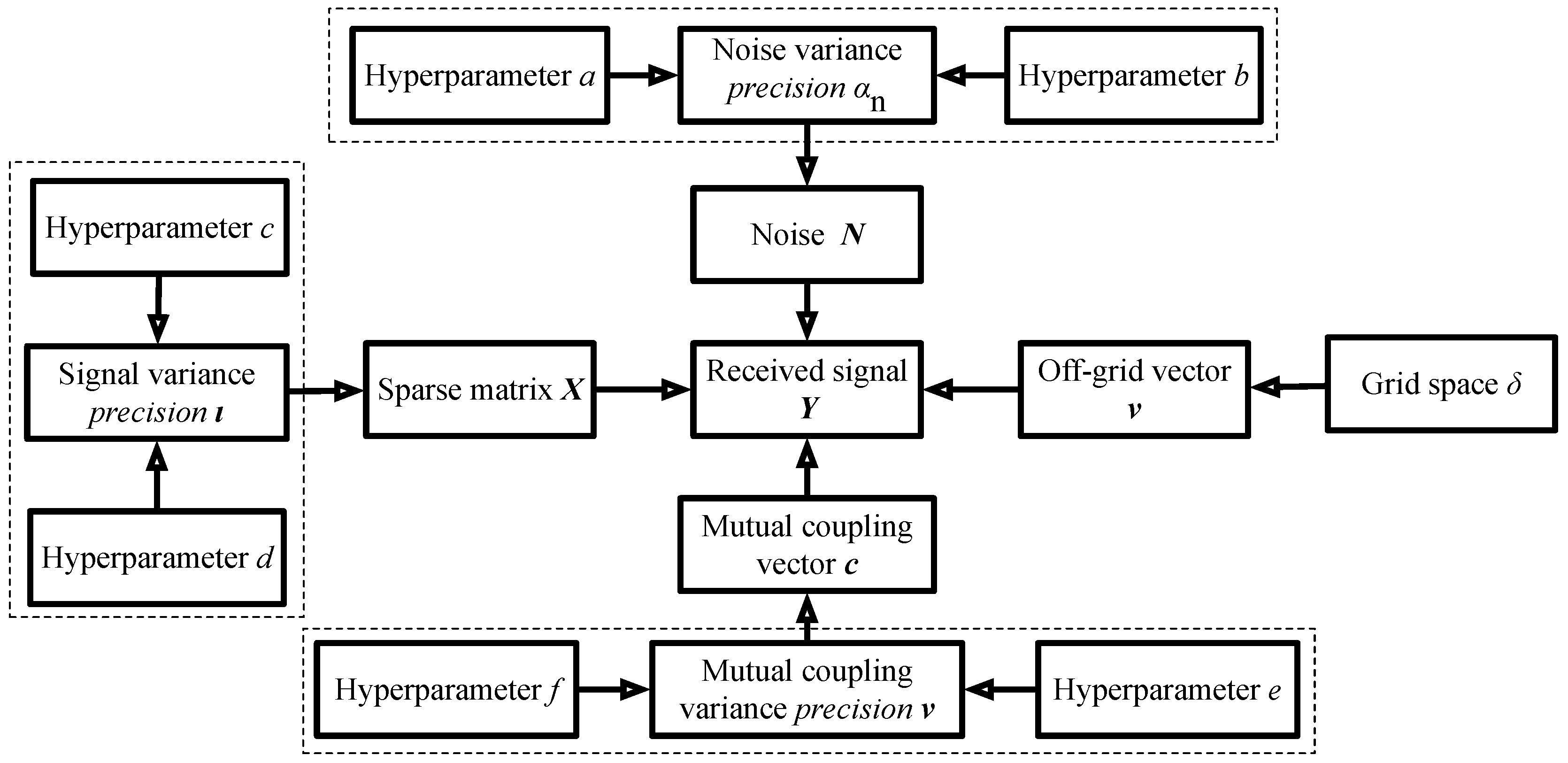
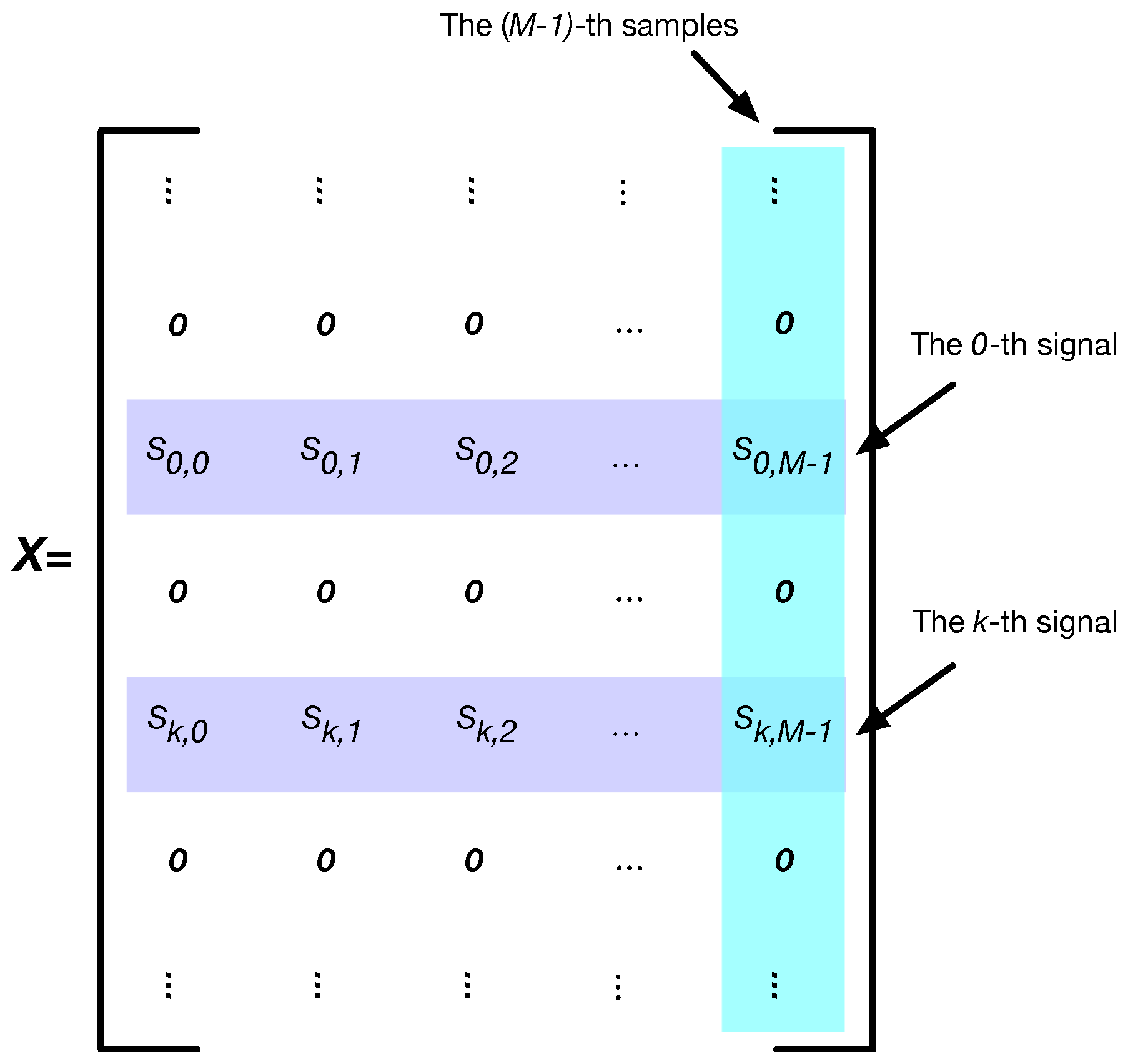
3.1. Sparse-Based Signal Model

Since the received signals are sparse in the spatial domain, we propose a sparse-based model to estimate the directions with unknown mutual coupling effect. In the sparse-based model, the dictionary matrix must be established first, so an over-complete dictionary matrix can be formulated by discretizing the signal direction uniformly in the spatial domain

$$\begin{array}{c}\hfill \mathit{D}\triangleq \left[\begin{array}{c}\mathit{Q}\left({\zeta }_0\right),\mathit{Q}\left({\zeta }_1\right),\dots ,\mathit{Q}\left({\zeta }_{U-1}\right)\end{array}\right]\in {\mathbb{C}}^{N\times UN},\end{array}$$

(10)

where ${\zeta }_u$ denotes the u-th discretized direction ($u=0,1,\dots ,U-1$), U denotes the number of discretized directions, the grid size is defined as $\delta \triangleq |{\zeta }_{u+1}-{\zeta }_u|$, and we use a vector to contain all the discretized directions $\mathbf{\zeta }\triangleq \left[\begin{array}{c}{\zeta }_0,{\zeta }_1,\dots ,{\zeta }_{U-1}\end{array}\right]$.

With the discretized directions and the system model in (9), a sparse-based on-grid direction finding model can be expressed as

$$\begin{array}{c}\hfill \mathit{Y}=\mathit{D}(\mathit{X}\otimes \mathit{c})+\mathit{n},\end{array}$$

(11)

where $\mathit{X}$ is a sparse matrix

$$\begin{array}{c}\hfill \mathit{X}\triangleq \left[\begin{array}{c}{\mathit{x}}_0,{\mathit{x}}_1,\dots ,{\mathit{x}}_{M-1}\end{array}\right]\in {\mathbb{C}}^{U\times M}.\end{array}$$

(12)

The structure of sparse matrix $\mathit{X}$ is shown in Figure 2, and the sparse vectors (${\mathit{x}}_0$, ${\mathit{x}}_1$, …, ${\mathit{x}}_{M-1}$) have the same support sets. When the direction of the k-th received signal ${\theta }_k$ is equal to the $u_k$-th discretized direction ${\zeta }_{u_k}$, we have $X_{u_k,m}=S_{k,m}$, so the u-th row and m-th column of $\mathit{X}$ is

$$\begin{array}{c}\hfill X_{u,m}=\left\{\begin{array}{ll}{S}_{k,m},\hfill & u=u_k\hfill \\ 0,\hfill & \mathrm{otherwise}\hfill \end{array}\right..\end{array}$$

(13)

The sparse-based model in (12) assumes that the directions of received signals are exactly on the discretized grids. However, in the practical direction finding system, when the direction ${\theta }_k$ is not on the discretized grids, the direction ${\theta }_k$ can be represented by ${\zeta }_{u_k}$, which is a grid nearest to ${\theta }_k$. Thus, the corresponding matrix $\mathit{Q}\left({\theta }_k\right)$ in (2) can be approximated by

$$\begin{array}{c}\hfill \mathit{Q}\left({\theta }_k\right)\approx \mathit{Q}\left({\zeta }_{u_k}\right)+({\theta }_k-{\zeta }_{u_k})\Omega \left({\zeta }_{u_k}\right),\end{array}$$

(14)

where the first-order derivative is defined as $\Omega \left({\zeta }_{u_k}\right)\triangleq {\left.\frac{\partial \mathit{Q}\left(\zeta \right)}{\partial \zeta }\right|}_{\zeta ={\zeta }_{u_k}}$. For example, as shown in Figure 3, the direction of signal $s_k\left(t\right)$ is ${\theta }_k$, and the nearest grid is ${\zeta }_3$. Thus, the corresponding matrix $\mathit{Q}\left({\theta }_k\right)$ in (14) can be written as $\mathit{Q}\left({\theta }_k\right)\approx \mathit{Q}\left({\zeta }_3\right)+({\theta }_k-{\zeta }_3)\Omega \left({\zeta }_3\right)$.

Therefore, with the approximation in (14), the received signal in (9) can be approximated by a sparse-based off-grid model

$$\begin{array}{c}\hfill \mathit{Y}\approx \mathbf{\Psi }\left(\mathbf{\nu }\right)(\mathit{X}\otimes \mathit{c})+\mathit{N},\end{array}$$

(15)

where $\mathbf{\Psi }\left(\mathbf{\nu }\right)\triangleq \mathit{D}+\mathbf{\Xi }\left(diag\left\{\mathbf{\nu }\right\}\otimes {\mathit{I}}_N\right)$, $\mathbf{\Xi }\triangleq \left[\begin{array}{c}{\mathbf{\Xi }}_0,{\mathbf{\Xi }}_1,\dots ,{\mathbf{\Xi }}_{U-1}\end{array}\right]$, and the u-th submatrix of $\mathbf{\Xi }$ is denoted as ${\mathbf{\Xi }}_u\triangleq \Omega \left({\zeta }_u\right)$. Additionally, a vector $\mathbf{\nu }\in {\mathbb{R}}^{U\times 1}$ is used to represent the off-grid directions, and the u-th entry is

$$\begin{array}{c}\hfill {\nu }_u=\left\{\begin{array}{ll}{\theta }_k-{\zeta }_{u_k},\hfill & u=u_k\hfill \\ 0,\hfill & \mathrm{otherwise}\hfill \end{array}\right..\end{array}$$

(16)

Finally, an off-grid sparse-based model is formulated for the direction finding problem in (15). We will estimate the directions by reconstructing the sparse matrix $\mathit{X}$. The positions of non-zero entries in $\mathit{X}$ indicate the directions of received signals. Simultaneously, the unknown parameters including the mutual coupling vector $\mathit{c}$, the noise variance ${\sigma }_{\mathrm{n}}^2$ and the off-grid vector $\mathbf{\nu }$ will also be estimated.

3.2. Distribution Assumptions

In the proposed DFSMC method, the sparse Bayesian learning theory is adopted, and the method is established based on the distribution assumptions of all the unknown parameters. We assume that the unknown parameters follow the following distributions:

• Noise $\mathit{N}$: Gaussian distribution;
• The precision of noise variance ${\alpha }_{\mathrm{n}}$: Gamma distribution;
• Sparse matrix $\mathit{X}$: Gaussian distribution;
• The precision of signal variance $\mathbf{\iota }$: Gamma distribution;
• Mutual coupling vector $\mathit{c}$: Gaussian distribution;
• The precision of mutual coupling variance $\mathbf{\vartheta }$: Gamma distribution;
• Off-grid vector $\mathbf{\nu }$: Uniform distribution.

The relationships between all the unknown parameters are given in Figure 4, and we will describe the distributions more clear in the following contents.

3.2.1. The Distribution of Noise

When the received signals are independent between different samples, with the assumption of circular symmetric white Gaussian noise, the distribution of noise can be expressed as

$$\begin{array}{c}\hfill p\left(\mathit{N}\right|{\sigma }_{\mathrm{n}}^2)={\displaystyle \prod _{m=0}^{M-1}}\mathcal{CN}\left({\mathit{n}}_m\right|{\mathbf{0}}_{N\times 1},{\sigma }_{\mathrm{n}}^2{\mathit{I}}_N),\end{array}$$

(17)

where ${\sigma }_{\mathrm{n}}^2$ denotes the noise variance, and the complex Gaussian distribution with the mean being $\mathbf{\mu }$ and the covariance matrix being $\mathbf{\Sigma }$ is expressed as

$$\begin{array}{c}\hfill \mathcal{CN}\left(\mathit{x}\right|\mathbf{\mu },\mathbf{\Sigma })=\frac{1}{{\pi }^{N}det(\mathbf{\Sigma })}{e}^{-{(\mathit{x}-\mathbf{\mu })}^{\mathrm{H}}{\mathbf{\Sigma }}^{-1}(\mathit{x}-\mathbf{\mu })}.\end{array}$$

(18)

3.2.2. The Distribution of Noise Variance ${\sigma }_{\mathrm{n}}^2$

In this paper, the noise variance is unknown. Since the Gamma distribution is a conjugate prior of Gaussian distribution, the posterior distribution also follows a Gamma distribution. Therefore, using the Gamma distribution can simplify the following analysis. With the unknown noise variance ${\sigma }_{\mathrm{n}}^2$, we use a Gamma distribution to describe the precision of noise variance ${\alpha }_{\mathrm{n}}\triangleq {\sigma }_{\mathrm{n}}^{-2}$, and we have the following Gamma distribution

$$\begin{array}{c}\hfill p\left({\alpha }_{\mathrm{n}}\right)=g({\alpha }_{\mathrm{n}};a,b),\end{array}$$

(19)

where a and b are the hyperparameters for ${\alpha }_{\mathrm{n}}$, and $g({\alpha }_{\mathrm{n}};a,b)\triangleq {\Gamma }^{-1}\left(a\right)b^a{\alpha }_{\mathrm{n}}^{a-1}{e}^{-b{\alpha }_{\mathrm{n}}}$, $\Gamma \left(a\right)\triangleq {\int }_0^{\infty }{x}^{a-1}{e}^{-x}dx$.

3.2.3. The Distribution of Sparse Matrix

With the independent received signals $\mathit{S}$ among samples, we can assume that the sparse matrix $\mathit{X}$ follows a zero-mean Gaussian distribution

$$\begin{array}{c}\hfill p\left(\mathit{X}\right|{\mathbf{\Lambda }}_{\mathrm{x}})={\displaystyle \prod _{m=0}^{M-1}}\mathcal{CN}\left({\mathit{x}}_m\right|{\mathbf{0}}_{U\times 1},{\mathbf{\Lambda }}_{\mathrm{x}}),\end{array}$$

(20)

where the covariance matrix ${\mathbf{\Lambda }}_{\mathrm{x}}\in {\mathbb{R}}^{U\times U}$ is a diagonal matrix with the u-th diagonal entry being ${\sigma }_{\mathrm{x},u}^2$.

3.2.4. The Distribution of Signal Variance

Similarity, with the unknown signal variance ${\mathbf{\Lambda }}_{\mathrm{x}}$, we define the precision vector $\mathbf{\iota }\triangleq {\left[\begin{array}{c}{\iota }_0,{\iota }_1,\dots ,{\iota }_{U-1}\end{array}\right]}^{\mathrm{T}}$, where ${\iota }_u\triangleq {\sigma }_{x,u}^{-2}$, so $\mathbf{\iota }$ can be expressed by a Gamma prior

$$\begin{array}{c}\hfill p(\mathbf{\iota };c,d)={\displaystyle \prod _{u=0}^{U-1}}g({\iota }_u;c,d),\end{array}$$

(21)

where c and d are the hyperparmaters for $\mathbf{\iota }$.

3.2.5. The Distribution of Mutual Coupling Vector

With the unknown mutual coupling vector, when the mutual coupling coefficients are independent between antennas, the distribution of mutual coupling vector $\mathit{c}$ can be expressed as a Gaussian distribution

$$\begin{array}{cc}\hfill p\left(\mathit{c}\right|{\mathbf{\Lambda }}_{\mathrm{c}})& ={\displaystyle \prod _{n=0}^{N-1}}\mathcal{CN}\left(c_n\right|0,{\mathbf{\Lambda }}_{\mathrm{c}}),\hfill \end{array}$$

(22)

where the covariance matrix ${\mathbf{\Lambda }}_{\mathrm{c}}\in {\mathbb{R}}^{N\times N}$ is a diagonal matrix with the n-th diagonal entry being ${\sigma }_{c,n}^2$.

3.2.6. The Distribution of Mutual Coupling Variance

By defining the precisions $\mathbf{\vartheta }\triangleq {\left[\begin{array}{c}{\vartheta }_0,{\vartheta }_1,\dots ,{\vartheta }_{N-1}\end{array}\right]}^{\mathrm{T}}$ (${\vartheta }_n\triangleq {\sigma }_{c,n}^{-2}$), we use a Gamma distribution to describe the distribution of $\mathbf{\vartheta }$

$$\begin{array}{cc}\hfill p(\mathbf{\vartheta };e,f)& ={\displaystyle \prod _{n=0}^{N-1}}g({\vartheta }_n;e,f),\hfill \end{array}$$

(23)

where both e and f are the hyperparameters of $\mathbf{\vartheta }$.

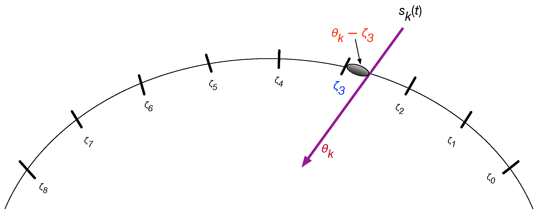
3.2.7. The Distribution of Off-Grid Vector

We can assume that the off-grid vector $\mathbf{\nu }$ follows a uniform distribution, and the distribution of ${\nu }_u$ can be expressed as

$$\begin{array}{c}\hfill p({\nu }_u;\delta )=U_{{\nu }_u}\left(\left[-\frac{1}{2}\delta ,\frac{1}{2}\delta \right]\right),\end{array}$$

(24)

where the uniform distribution is defined as

$$\begin{array}{c}\hfill {\mathcal{U}}_x\left(\left[a,b\right]\right)\triangleq \left\{\begin{array}{cc}\frac{1}{b-a},\hfill & a\le x\le b\hfill \\ 0,\hfill & \mathrm{otherwise}\hfill \end{array}\right..\end{array}$$

(25)

3.3. DFSMC Method

With the distribution assumptions of unknown parameters, a novel direction finding method based on the SBL is proposed with the unknown mutual coupling effect, named DFSMC. In the SBL-based method, the posterior probabilities for all the unknown parameters are theoretically derived.

To estimate the directions, we formulate the following problem to maximize the posterior probability

$$\begin{array}{c}\hfill \hat{\wp }=arg\underset{\wp }{max}p\left(\wp \right|\mathit{Y}),\end{array}$$

(26)

where a set $\wp \triangleq \left\{\mathit{X},\mathbf{\nu },\mathit{c},{\sigma }_{\mathrm{n}}^2,\mathbf{\iota },\mathbf{\vartheta }\right\}$ is used to contain all the unknown parameters. However, the problem (26) is too complex and cannot be solved directly. The expectation maximum (EM)-based method is used to realize the proposed DFSMC method. Additionally, with the received signal $\mathit{Y}$, the joint distribution with unknown parameters can be expressed as

$$\begin{array}{cc}\hfill p(\mathit{Y},\wp )& =p\left(\mathit{Y}\right|\wp )p\left(\mathit{X}\right|\mathbf{\iota })p\left(\mathit{c}\right|\mathbf{\vartheta })p\left({\alpha }_{\mathrm{n}}\right)p\left(\mathbf{\iota }\right)p\left(\mathbf{\vartheta }\right)p\left(\mathbf{\nu }\right).\hfill \end{array}$$

(27)

The details to estimate all unknown parameters are given as follows.

3.3.1. The Sparse Matrix

Given the received signal $\mathit{Y}$ and the parameters $(\wp \setminus \mathit{X})$ excepting $\mathit{X}$, the the posterior of $\mathit{X}$ can be expressed as

$$\begin{array}{cc}\hfill p\left(\mathit{X}\right|\mathit{Y},\mathbf{\nu },\mathit{c},{\alpha }_{\mathrm{n}},\mathbf{\iota },\mathbf{\vartheta })& =\frac{p\left(\mathit{Y}\right|\wp \left)p\right(\mathit{X}\left|\mathbf{\iota }\right)}{p\left(\mathit{Y}\right|\mathbf{\nu },\mathit{c},{\alpha }_{\mathrm{n}},\mathbf{\iota },\mathbf{\vartheta })}\propto p\left(\mathit{Y}\right|\wp )p\left(\mathit{X}\right|\mathbf{\iota }),\hfill \end{array}$$

(28)

where both $p\left(\mathit{Y}\right|\wp )$ and $p\left(\mathit{X}\right|\mathbf{\iota })$ follow Gaussian distributions, and can be calculated as

$$\begin{array}{cc}\hfill p\left(\mathit{Y}\right|\wp )& ={\displaystyle \prod _{m=0}^{M-1}}\frac{{\alpha }_{\mathrm{n}}^N}{{\pi }^N}{e}^{-{\alpha }_{\mathrm{n}}{\parallel {\mathit{y}}_m-\mathbf{\Psi }\left(\mathbf{\nu }\right)({\mathit{x}}_m\otimes \mathit{c})\parallel }_2^2},\hfill \end{array}$$

(29)

$$\begin{array}{cc}\hfill p\left(\mathit{X}\right|\mathbf{\iota })& ={\displaystyle \prod _{m=0}^{M-1}}\left({\displaystyle \prod _{u=0}^{U-1}}{\iota }_u\right)\frac{1}{{\pi }^U}{e}^{-{\mathit{x}}_m^{\mathrm{H}}diag\left\{\mathbf{\iota }\right\}{\mathit{x}}_m}.\hfill \end{array}$$

(30)

Therefore, the posterior of $\mathit{X}$ is also a Gaussian function

$$p\left(\mathit{X}\right|\mathit{Y},\mathbf{\nu },\mathit{c},{\alpha }_{\mathrm{n}},\mathbf{\iota },\mathbf{\vartheta })={\displaystyle \prod _{m=0}^{M-1}}\mathcal{CN}\left({\mathit{x}}_m\right|{\mathbf{\mu }}_m,{\mathbf{\Sigma }}_{\mathrm{X}}),$$

(31)

where the mean ${\mathbf{\mu }}_m$ and covariance matrix ${\mathbf{\Sigma }}_{\mathrm{X}}$ are obtained from (29) and (30) as

$$\begin{array}{cc}\hfill {\mathbf{\mu }}_m& ={\alpha }_{\mathrm{n}}^{\mathrm{H}}{\mathbf{\Sigma }}_{\mathrm{X}}^{\mathrm{H}}{\mathfrak{T}}^H(\mathbf{\nu },\mathit{c}){\mathit{y}}_m,\hfill \end{array}$$

(32)

$$\begin{array}{cc}\hfill {\mathbf{\Sigma }}_{\mathrm{X}}& ={\left[{\alpha }_{\mathrm{n}}{\mathfrak{T}}^H(\mathbf{\nu },\mathit{c})\mathfrak{T}(\mathbf{\nu },\mathit{c})+diag\left\{\mathbf{\iota }\right\}\right]}^{-1}\hfill \end{array}$$

(33)

and we define the following function

$$\begin{array}{c}\hfill \mathfrak{T}(\mathbf{\nu },\mathit{c})\triangleq \mathbf{\Psi }\left(\mathbf{\nu }\right)({\mathit{I}}_U\otimes \mathit{c}).\end{array}$$

(34)

Additionally, to simplify the notations, the u-th entry of ${\mathbf{\mu }}_m$ is denoted as ${\mu }_{u,m}$, and we can collect all the mean ${\mathbf{\mu }}_m$ as a matrix $\mathbf{\mu }\triangleq \left[\begin{array}{c}{\mathbf{\mu }}_0,{\mathbf{\mu }}_1,\dots ,{\mathbf{\mu }}_{M-1}\end{array}\right]$.

To estimate the other unknown parameters $\wp \setminus \mathit{X}$, with (27), we can formulate the following likelihood function

$$\begin{array}{c}\hfill \mathcal{L}(\mathbf{\nu },\mathit{c},{\alpha }_{\mathrm{n}},\mathbf{\iota },\mathbf{\vartheta })=\mathcal{E}\{lnp\left(\mathit{Y}\right|\wp )p\left(\mathit{X}\right|\mathbf{\iota })p\left(\mathit{c}\right|\mathbf{\vartheta })p\left({\alpha }_{\mathrm{n}}\right)p\left(\mathbf{\iota }\right)p\left(\mathbf{\vartheta }\right)p\left(\mathbf{\nu }\right)\}.\end{array}$$

(35)

where we just use $\mathcal{E}\left\{·\right\}$ to represent ${\mathcal{E}}_{\mathit{X}|\mathit{Y},\mathbf{\nu },{\alpha }_{\mathrm{n}},\mathbf{\iota },\mathbf{\vartheta }}\left\{·\right\}$. Thus, the EM-based method can be used to estimate $\wp \setminus \mathit{X}$, and the details are given in the following contents. Additionally, the derivatives for the complex vector and matrix are given as the following lemma.

Lemma 1.

With both the complex vectors ($\mathit{u}\in {\mathbb{C}}^{P\times 1}$,$\mathit{v}\in {\mathbb{C}}^{P\times 1}$) and the complex matrix$\mathit{A}\in {\mathbb{C}}^{M\times P}$being the function of a complex vector$\mathit{x}\in {\mathbb{C}}^{N\times 1}$, the following derivations can be obtained

$$\begin{array}{c}\frac{\partial {\mathit{u}}^H\mathit{v}}{\partial \mathit{x}}={\mathit{v}}^T\frac{\partial \left({\mathit{u}}^{\ast }\right)}{\partial \mathit{x}}+{\mathit{u}}^H\frac{\partial \mathit{v}}{\partial \mathit{x}},\hfill \end{array}$$

(36)

$$\begin{array}{c}\frac{\partial \mathit{Au}}{\partial \mathit{x}}=\left[\begin{array}{c}\frac{\partial \mathit{A}}{\partial x_0}\mathit{u}+\mathit{A}\frac{\partial \mathit{u}}{\partial x_0},\dots ,\frac{\partial \mathit{A}}{\partial x_n}\mathit{u}+\mathit{A}\frac{\partial \mathit{u}}{\partial x_n},\dots \end{array}\right].\hfill \end{array}$$

(37)

Proof. 

See: Appendix A. □

3.3.2. The Mutual Coupling Vector

Ignoring terms independent thereof in $\mathcal{L}(\mathbf{\nu },\mathit{c},{\alpha }_{\mathrm{n}},\mathbf{\iota },\mathbf{\vartheta })$, we can obtain the following likelihood function for the mutual coupling vector $\mathit{c}$

$$\begin{array}{cc}\hfill \mathcal{L}& \left(\mathit{c}\right)=\mathcal{E}\left\{lnp\left(\mathit{Y}\right|\mathit{X},\mathbf{\nu },\mathit{c},{\alpha }_{\mathrm{n}})p\left(\mathit{c}\right|\mathbf{\vartheta })\right\}\hfill \\ & =\mathcal{E}\left\{ln{\displaystyle \prod _{m=0}^{M-1}}\mathcal{CN}\left({\mathit{y}}_m\right|\mathbf{\Psi }\left(\mathbf{\nu }\right)({\mathit{x}}_m\otimes \mathit{c}),{\alpha }_{\mathrm{n}}^{-1}{\mathit{I}}_N)\right\}+ln{\displaystyle \prod _{n=0}^{N-1}}\mathcal{CN}\left(c_n\right|0,{\vartheta }_n^{-1})\hfill \\ & \propto -{\alpha }_{\mathrm{n}}M{\mathcal{G}}_1(\mathit{c},\mathbf{\nu })-{\displaystyle \sum _{m=0}^{M-1}}{\alpha }_{\mathrm{n}}{\mathcal{G}}_{2,m}(\mathit{c},\mathbf{\nu })-{\mathcal{G}}_3\left(\mathit{c}\right),\hfill \end{array}$$

(38)

where we have

$$\begin{array}{cc}\hfill \mathcal{E}\left\{lnp\left(\mathit{Y}\right|\mathit{X},\mathbf{\nu },\mathit{c},{\alpha }_{\mathrm{n}})\right\}=& MNln\frac{{\alpha }_{\mathrm{n}}}{\pi }-{\alpha }_{\mathrm{n}}M{\mathcal{G}}_1(\mathit{c},\mathbf{\nu })-{\displaystyle \sum _{m=0}^{M-1}}{\alpha }_{\mathrm{n}}{\mathcal{G}}_{2,m}(\mathit{c},\mathbf{\nu }),\hfill \end{array}$$

(39)

and ${\mathcal{G}}_1(\mathit{c},\mathbf{\nu })\triangleq Tr\left\{{\mathfrak{T}}^H(\mathbf{\nu },\mathit{c})\mathfrak{T}(\mathbf{\nu },\mathit{c}){\mathbf{\Sigma }}_{\mathrm{X}}\right\}$, ${\mathcal{G}}_{2,m}(\mathit{c},\mathbf{\nu })\triangleq {\parallel {\mathit{y}}_m-\mathbf{\Psi }\left(\mathbf{\nu }\right)({\mathbf{\mu }}_m\otimes \mathit{c})\parallel }_2^2$, ${\mathcal{G}}_3\left(\mathit{c}\right)\triangleq {\sum }_{n=0}^{N-1}{\vartheta }_n{\left|c_n\right|}^2$.

To estimate the mutual coupling vector $\mathit{c}$, we can maximize the likelihood function $\mathcal{L}\left(\mathit{c}\right)$, and we have

$$\begin{array}{c}\hfill \hat{\mathit{c}}=arg\underset{\mathit{c}}{max}\mathcal{L}\left(\mathit{c}\right).\end{array}$$

(40)

Therefore, by setting $\frac{\partial \mathcal{L}\left(\mathit{c}\right)}{\partial \mathit{c}}=\mathbf{0}$, the mutual coupling vector can be obtained. We can calculate

$$\begin{array}{cc}\hfill \frac{\partial \mathcal{L}\left(\mathit{c}\right)}{\partial \mathit{c}}& =-{\alpha }_{\mathrm{n}}M\frac{\partial {\mathcal{G}}_1(\mathit{c},\mathbf{\nu })}{\partial \mathit{c}}-{\displaystyle \sum _{m=0}^{M-1}}{\alpha }_{\mathrm{n}}\frac{\partial {\mathcal{G}}_{2,m}(\mathit{c},\mathbf{\nu })}{\partial \mathit{c}}-\frac{\partial {\mathcal{G}}_3\left(\mathit{c}\right)}{\partial \mathit{c}}.\hfill \end{array}$$

(41)

In (41), $\frac{\partial {\mathcal{G}}_1(\mathit{c},\mathbf{\nu })}{\partial \mathit{c}}$, $\frac{\partial {\mathcal{G}}_{2,m}(\mathit{c},\mathbf{\nu })}{\partial \mathit{c}}$ and $\frac{\partial {\mathcal{G}}_3\left(\mathit{c}\right)}{\partial \mathit{c}}$ can be calculated as follows.

• For $\frac{\partial {\mathcal{G}}_1(\mathit{c},\mathbf{\nu })}{\partial \mathit{c}}$: With the derivations of complex vector and matrix in Appendix A, $\frac{\partial {\mathcal{G}}_1(\mathit{c},\mathbf{\nu })}{\partial \mathit{c}}$ is a row vector, and the n-th entry can be calculated as

  $$\begin{array}{c}{\left[\frac{\partial {\mathcal{G}}_1(\mathit{c},\mathbf{\nu })}{\partial \mathit{c}}\right]}_n=Tr\left\{\frac{\partial {\mathfrak{T}}^H(\mathbf{\nu },\mathit{c})\mathfrak{T}(\mathbf{\nu },\mathit{c}){\mathbf{\Sigma }}_{\mathrm{X}}}{\partial c_n}\right\}.\hfill \end{array}$$

  (42)
  Additionally, we can calculate

  $$\begin{array}{l}\frac{\partial {\mathfrak{T}}^H(\mathbf{\nu },\mathit{c})\mathfrak{T}(\mathbf{\nu },\mathit{c}){\mathbf{\Sigma }}_{\mathrm{X}}}{\partial c_n}=\frac{\partial {({\mathit{I}}_U\otimes \mathit{c})}^{\mathrm{H}}}{\partial c_n}{\mathbf{\Psi }}^{\mathrm{H}}\left(\mathbf{\nu }\right)\mathfrak{T}(\mathbf{\nu },\mathit{c}){\mathbf{\Sigma }}_{\mathrm{X}}]+{\mathfrak{T}}^H(\mathbf{\nu },\mathit{c})\mathbf{\Psi }\left(\mathbf{\nu }\right)\frac{\partial ({\mathit{I}}_U\otimes \mathit{c})}{\partial c_n}{\mathbf{\Sigma }}_{\mathrm{X}}\hfill \\ ={\mathfrak{T}}^H(\mathbf{\nu },\mathit{c})\mathbf{\Psi }\left(\mathbf{\nu }\right)\left({\mathit{I}}_U\otimes \frac{\partial \mathit{c}}{\partial c_n}\right){\mathbf{\Sigma }}_{\mathrm{X}}={\mathfrak{T}}^H(\mathbf{\nu },\mathit{c})\mathfrak{T}(\mathbf{\nu },{\mathit{e}}_n^N){\mathbf{\Sigma }}_{\mathrm{X}},\hfill \end{array}$$

  (43)

  where ${\mathit{e}}_n^N$ is a $N\times 1$ vector with the n-th entry being 1 and other entries being 0. Therefore, the n-th entry in (42) can be simplified as

  $$\begin{array}{cc}\hfill {\left[\frac{\partial {\mathcal{G}}_1(\mathit{c},\mathbf{\nu })}{\partial \mathit{c}}\right]}_n& ={\mathit{c}}^{\mathrm{H}}\left({\displaystyle \sum _{p=0}^{U-1}}{\displaystyle \sum _{k=0}^{U-1}}{\mathbf{\Psi }}_p^{\mathrm{H}}\left(\mathbf{\nu }\right){\mathbf{\Psi }}_k\left(\mathbf{\nu }\right){\Sigma }_{\mathrm{X},k,p}\right){\mathit{e}}_n^N,\hfill \end{array}$$

  (44)

  and we finally have the derivation of ${\mathcal{G}}_1(\mathit{c},\mathbf{\nu })$ as

  $$\begin{array}{cc}\hfill \frac{\partial {\mathcal{G}}_1(\mathit{c},\mathbf{\nu })}{\partial \mathit{c}}& ={\mathit{c}}^{\mathrm{H}}\left({\displaystyle \sum _{p=0}^{U-1}}{\displaystyle \sum _{k=0}^{U-1}}{\mathbf{\Psi }}_p^{\mathrm{H}}\left(\mathbf{\nu }\right){\mathbf{\Psi }}_k\left(\mathbf{\nu }\right){\Sigma }_{\mathrm{X},k,p}\right).\hfill \end{array}$$
• $\frac{\partial {\mathcal{G}}_{2,m}(\mathit{c},\mathbf{\nu })}{\partial \mathit{c}}$ can be simplified as

  $$\begin{array}{cc}\hfill \frac{\partial {\mathcal{G}}_{2,m}(\mathit{c},\mathbf{\nu })}{\partial \mathit{c}}& =-{[{\mathit{y}}_m-\mathbf{\Psi }\left(\mathbf{\nu }\right)({\mathbf{\mu }}_m\otimes \mathit{c})]}^{\mathrm{H}}\mathbf{\Psi }\left(\mathbf{\nu }\right)\frac{\partial {\mathbf{\mu }}_m\otimes \mathit{c}}{\partial \mathit{c}}\hfill \\ & =-{[{\mathit{y}}_m-\mathbf{\Psi }\left(\mathbf{\nu }\right)({\mathbf{\mu }}_m\otimes \mathit{c})]}^{\mathrm{H}}\mathbf{\Psi }\left(\mathbf{\nu }\right)({\mathbf{\mu }}_m\otimes {\mathit{I}}_N).\hfill \end{array}$$

  (45)
• $\frac{\partial {\mathcal{G}}_3\left(\mathit{c}\right)}{\partial \mathit{c}}$ can be simplified as $\frac{\partial {\mathcal{G}}_3\left(\mathit{c}\right)}{\partial \mathit{c}}={\mathit{c}}^{H}diag\left\{\mathbf{\vartheta }\right\}$.

Therefore, with (41), the mutual coupling vector can be finally estimated as

$$\begin{array}{c}\hfill \hat{\mathit{c}}={\mathit{H}}^{-1}\mathit{z},\end{array}$$

(46)

where

$$\begin{array}{cc}\hfill \mathit{H}& ={\displaystyle \sum _{m=0}^{M-1}}{\alpha }_{\mathrm{n}}{\mathfrak{P}}^H(\mathbf{\nu },{\mathbf{\mu }}_m)\mathfrak{P}(\mathbf{\nu },{\mathbf{\mu }}_m)+{\alpha }_{\mathrm{n}}M{\left({\displaystyle \sum _{p=0}^{U-1}}{\displaystyle \sum _{k=0}^{U-1}}{\mathbf{\Psi }}_p^{\mathrm{H}}\left(\mathbf{\nu }\right){\mathbf{\Psi }}_k\left(\mathbf{\nu }\right){\Sigma }_{\mathrm{X},k,p}\right)}^{\mathrm{H}}+diag\left\{\mathbf{\vartheta }\right\},\hfill \end{array}$$

(47)

$$\begin{array}{cc}\hfill \mathit{z}& ={\displaystyle \sum _{m=0}^{M-1}}{\alpha }_{\mathrm{n}}{\mathfrak{P}}^H(\mathbf{\nu },{\mathbf{\mu }}_m){\mathit{y}}_m,\hfill \end{array}$$

(48)

and we define $\mathfrak{P}(\mathbf{\nu },{\mathbf{\mu }}_m)\triangleq \mathbf{\Psi }\left(\mathbf{\nu }\right)({\mathbf{\mu }}_m\otimes {\mathit{I}}_N)$.

3.3.3. For the Precision of Signal Variance

Ignoring terms independent thereof in $\mathcal{L}(\mathbf{\nu },\mathit{c},{\alpha }_{\mathrm{n}},\mathbf{\iota },\mathbf{\vartheta })$, we can obtain the likelihood function of $\mathbf{\iota }$ as

$$\begin{array}{cc}\hfill \mathcal{L}\left(\mathbf{\iota }\right)=& \mathcal{E}\left\{lnp\left(\mathit{X}\right|\mathbf{\iota }\left)p\right(\mathbf{\iota })\right\}=\mathcal{E}\left\{ln{\displaystyle \prod _{m=0}^{M-1}}\mathcal{CN}\left({\mathit{x}}_m\right|{\mathbf{0}}_{U\times 1},{\mathbf{\Lambda }}_{\mathrm{x}})\right\}+ln{\displaystyle \prod _{u=0}^{U-1}}g({\iota }_u;c,d).\hfill \end{array}$$

(49)

Then, the precision of signal variance can be estimated by $\hat{\mathbf{\iota }}=arg{max}_{\mathbf{\iota }}\mathcal{L}\left(\mathbf{\iota }\right)$.

By setting $\frac{\partial \mathcal{L}\left(\mathbf{\iota }\right)}{\partial \mathbf{\iota }}=0$, the u-th entry of $\mathbf{\iota }$ can be obtained as

$$\begin{array}{c}\hfill {\hat{\iota }}_u=\frac{M+c-1}{d+M{\Sigma }_{\mathrm{X},u,u}+{\sum }_{m=0}^{M-1}{\left|{\mu }_{u,m}\right|}^2}.\end{array}$$

(50)

In the iterative algorithm, (50) can be rewritten as

$$\begin{array}{c}\hfill {\hat{\iota }}_u^{i+1}\approx \frac{M-1-{\hat{\iota }}_u^i{\sum }_{m=0}^{M-1}{\left|{\mu }_{u,m}\right|}^2}{d+M{\Sigma }_{\mathrm{X},u,u}},\end{array}$$

(51)

where ${\hat{\iota }}_u^{i+1}$ and ${\hat{\iota }}_u^i$ are the esitmated results at the $(i+1)$-th and the i-th iterations, respectively.

3.3.4. For ${\alpha }_{\mathrm{n}}$

Ignoring terms independent thereof in $\mathcal{L}(\mathbf{\nu },\mathit{c},{\alpha }_{\mathrm{n}},\mathbf{\iota },\mathbf{\vartheta })$, we can obtain the likelihood function

$$\begin{array}{cc}\hfill \mathcal{L}\left({\alpha }_{\mathrm{n}}\right)& =\mathcal{E}\left\{lnp\left(\mathit{Y}\right|\mathit{X},\mathbf{\nu },\mathit{c},{\alpha }_{\mathrm{n}})p\left({\alpha }_{\mathrm{n}}\right)\right\}\hfill \\ & =\mathcal{E}\left\{ln{\displaystyle \prod _{m=0}^{M-1}}\mathcal{CN}\left({\mathit{y}}_m|\mathbf{\Psi }\left(\mathbf{\nu }\right)({\mathit{x}}_m\otimes \mathit{c}),{\sigma }_{\mathrm{n}}^2\mathit{I}\right)\right\}+lng({\alpha }_{\mathrm{n}};a,b).\hfill \end{array}$$

(52)

The precision of noise variance can be estimated by

$$\begin{array}{c}\hfill {\hat{\alpha }}_{\mathrm{n}}=arg\underset{{\alpha }_{\mathrm{n}}}{max}\mathcal{L}\left({\alpha }_{\mathrm{n}}\right).\end{array}$$

(53)

By setting $\frac{\partial \mathcal{L}\left({\alpha }_{\mathrm{n}}\right)}{\partial {\alpha }_{\mathrm{n}}}=0$, we can obtain

$$\begin{array}{cc}\hfill {\hat{\alpha }}_{\mathrm{n}}& =\frac{MN+a-1}{M{\mathcal{G}}_1(\mathit{c},\mathbf{\nu })+{\sum }_{m=0}^{M-1}{\mathcal{G}}_{2,m}(\mathit{c},\mathbf{\nu })+b}.\hfill \end{array}$$

(54)

In the iterative algorithm, (54) can be rewritten as

$$\begin{array}{c}\hfill {\hat{\alpha }}_{\mathrm{n}}^{i+1}\approx \frac{MN-1-{\hat{\alpha }}_{\mathrm{n}}^i{\sum }_{m=0}^{M-1}{\mathcal{G}}_{2,m}(\mathit{c},\mathbf{\nu })}{M{\mathcal{G}}_1(\mathit{c},\mathbf{\nu })+b}.,\end{array}$$

(55)

where ${\hat{\alpha }}_{\mathrm{n}}^{i+1}$ and ${\hat{\alpha }}_{\mathrm{n}}^i$ are the esitmated results at the $(i+1)$-th and the i-th iterations, respectively.

3.3.5. For the Precision of Mutual Coupling Variance

Ignoring terms independent thereof in $\mathcal{L}(\mathbf{\nu },\mathit{c},{\alpha }_{\mathrm{n}},\mathbf{\iota },\mathbf{\vartheta })$, we can obtain the likelihood function

$$\begin{array}{cc}\hfill \mathcal{L}\left(\mathbf{\vartheta }\right)& =\mathcal{E}\left\{lnp\left(\mathit{c}\right|\mathbf{\vartheta }\left)p\right(\mathbf{\vartheta })\right\}=\mathcal{E}\left\{ln{\displaystyle \prod _{n=0}^{N-1}}\mathcal{CN}\left(c_n\right|0,{\vartheta }_n^{-1})\right\}+ln{\displaystyle \prod _{n=0}^{N-1}}g({\vartheta }_n;e,f).\hfill \end{array}$$

(56)

The precision of mutual coupling variance can be estimated by $\hat{\mathbf{\vartheta }}=arg{max}_{\mathbf{\vartheta }}\mathcal{L}\left(\mathbf{\vartheta }\right)$.

By setting $\frac{\partial \mathcal{L}\left(\mathbf{\vartheta }\right)}{\partial \mathbf{\vartheta }}=\mathbf{0}$, we can obtain the n-th entry of $\mathbf{\vartheta }$ as

$$\begin{array}{c}\hfill {\hat{\vartheta }}_n\approx \frac{1}{f+c_n^{\mathrm{H}}{c}_n}.\end{array}$$

(57)

3.3.6. For the Off-Grid Vector

Ignoring terms independent thereof in $\mathcal{L}(\mathbf{\nu },\mathit{c},{\alpha }_{\mathrm{n}},\mathbf{\iota },\mathbf{\vartheta })$, we can obtain the likelihood function

$$\begin{array}{c}\hfill \mathcal{L}\left(\mathbf{\nu }\right)=\mathcal{E}\left\{lnp\left(\mathit{Y}\right|\mathit{X},\mathbf{\nu },\mathit{c},{\alpha }_n)p\left(\mathbf{\nu }\right)\right\}\propto -M{\mathcal{G}}_1(\mathit{c},\mathbf{\nu })-{\displaystyle \sum _{m=0}^{M-1}}{\mathcal{G}}_{2,m}(\mathit{c},\mathbf{\nu }).\end{array}$$

(58)

The off-grid vector can be estimated by

$$\begin{array}{c}\hfill \hat{\mathbf{\nu }}=arg\underset{\mathbf{\nu }}{max}\mathcal{L}\left(\mathbf{\nu }\right).\end{array}$$

(59)

Then, $\frac{\partial {\mathcal{G}}_1(\mathit{c},\mathbf{\nu })}{\partial \mathbf{\nu }}\in {\mathbb{R}}^{1\times U}$ is a row vector, and the u-th entry is

$$\begin{array}{c}{\left[\frac{\partial {\mathcal{G}}_1(\mathit{c},\mathbf{\nu })}{\partial \mathbf{\nu }}\right]}_u=Tr\left\{\frac{\partial {\mathfrak{T}}^H(\mathbf{\nu },\mathit{c})\mathfrak{T}(\mathbf{\nu },\mathit{c}){\mathbf{\Sigma }}_{\mathrm{X}}}{\partial {\mathbf{\nu }}_u}\right\}\hfill \\ =Tr\left\{\left[\begin{array}{c}\mathbf{0},{\mathfrak{T}}^H(\mathbf{\nu },\mathit{c}){\mathbf{\Xi }}_u\mathit{c},\mathbf{0}\end{array}\right]{\mathbf{\Sigma }}_{\mathrm{X}}\right\}+Tr\left\{{\left[\begin{array}{c}\mathbf{0},{\mathfrak{T}}^H(\mathbf{\nu },\mathit{c}){\mathbf{\Xi }}_u\mathit{c},\mathbf{0}\end{array}\right]}^{\mathrm{H}}{\mathbf{\Sigma }}_{\mathrm{X}}\right\}\hfill \\ =2\mathcal{R}\left\{{\displaystyle \sum _{m=0}^{U-1}}{\mathit{c}}^{\mathrm{H}}{\mathbf{\Psi }}_m^{\mathrm{H}}\left(\mathbf{\nu }\right){\mathbf{\Xi }}_u\mathit{c}{\Sigma }_{\mathrm{X},u,m}\right\}=2\mathcal{R}\left\{{\left[{\mathfrak{T}}^H(\mathbf{\nu },\mathit{c}){\mathbf{\Xi }}_u\mathit{c}\right]}^H{\mathbf{\Sigma }}_{\mathrm{X},:,u}\right\}.\hfill \end{array}$$

(60)

$\frac{\partial {\mathcal{G}}_1(\mathit{c},\mathbf{\nu })}{\partial \mathbf{\nu }}$ can be simplified as

$$\begin{array}{c}\hfill \frac{\partial {\mathcal{G}}_1(\mathit{c},\mathbf{\nu })}{\partial \mathbf{\nu }}=2\mathcal{R}\left\{diag{\left\{{\mathbf{\Sigma }}_{\mathrm{X}}{\mathfrak{T}}^H(\mathbf{\nu },\mathit{c})\mathbf{\Xi }({\mathit{I}}_U\otimes \mathit{c})\right\}}^{\mathrm{T}}\right\}.\end{array}$$

(61)

Additionally, $\frac{\partial {\mathcal{G}}_{2,m}(\mathit{c},\mathbf{\nu })}{\partial \mathbf{\nu }}$ can be obtained as

$$\begin{array}{c}\frac{\partial {\mathcal{G}}_{2,m}(\mathit{c},\mathbf{\nu })}{\partial \mathbf{\nu }}=-2\mathcal{R}\left\{{[{\mathit{y}}_m-\mathbf{\Psi }\left(\mathbf{\nu }\right)({\mathbf{\mu }}_m\otimes \mathit{c})]}^{\mathrm{H}}\frac{\partial \mathbf{\Psi }\left(\mathbf{\nu }\right)({\mathbf{\mu }}_m\otimes \mathit{c})}{\partial \mathbf{\nu }}\right\}\hfill \\ =-2\mathcal{R}\left\{{[{\mathit{y}}_m-\mathbf{\Psi }\left(\mathbf{\nu }\right)({\mathbf{\mu }}_m\otimes \mathit{c})]}^{\mathrm{H}}\mathbf{\Xi }(diag\left\{{\mathbf{\mu }}_m\right\}\otimes \mathit{c})\right\}.\hfill \end{array}$$

(62)

Therefore, with $\frac{\partial \mathcal{L}\left(\mathbf{\nu }\right)}{\partial {\mathbf{\nu }}_u}=0$, we can obtain

$$\begin{array}{c}\hfill \hat{\mathbf{\nu }}={\mathit{G}}^{-1}\mathit{z},\end{array}$$

(63)

where the entry of the u-th row in $\mathit{G}\in {\mathbb{R}}^{U\times U}$ is

$$\begin{array}{cc}\hfill {\mathit{G}}_{u,:}=& \mathcal{R}\left\{M{\mathit{c}}^H{\mathbf{\Xi }}_u^H\mathbf{\Xi }(diag\left\{{\mathbf{\Sigma }}_{\mathrm{X},:,u}\right\}\otimes \mathit{c})\right\}+{\displaystyle \sum _{m=0}^{M-1}}\mathcal{R}\left\{{\mu }_{m,u}{\mathit{c}}^{\mathrm{T}}{\mathbf{\Xi }}_u^T{\mathbf{\Xi }}^{\ast }({\mathit{I}}_U\otimes {\mathit{c}}^{\ast }){diag}^{\ast }\left\{{\mathbf{\mu }}_m\right\}\right\},\hfill \end{array}$$

(64)

and the u-th entry of $\mathit{z}\in {\mathcal{R}}^{U\times 1}$ is

$$\begin{array}{cc}\hfill z_u& ={\displaystyle \sum _{m=0}^{M-1}}\mathcal{R}\left\{{[{\mathit{y}}_m-\mathit{D}({\mathbf{\mu }}_m\otimes \mathit{c})]}^{\mathrm{H}}{\mathbf{\Xi }}_u{\mu }_{m,u}\mathit{c}\right\}-M\mathcal{R}\left\{{\mathit{c}}^H{\mathbf{\Xi }}_u^H\mathit{D}({\mathit{I}}_U\otimes \mathit{c}){\mathbf{\Sigma }}_{\mathrm{X},:,u}\right\}.\hfill \end{array}$$

(65)

In Algorithm 1, we show the details of the proposed DFSMC method for the direction finding with the unknown mutual coupling effect. In the proposed DFSMC algorithm, after the iterations, we can obtain the spatial spectrum $P_X$ of the sparse matrix $\mathit{X}$ from the received signal $\mathit{Y}$. Then, by searching all the values of $P_X$, the corresponding peak values can be found. By selecting positions of peak values corresponding to the K maximum values, we can estimate the directions with $\mathbf{\zeta }+\mathbf{\nu }$.

Algorithm 1 DFSMC algorithm for direction finding with the unknown mutual coupling effect.

1: Input: received signal $\mathit{Y}$, the number of samples M, the numbers of iterations $N_1$, $N_2$ and $N_3$ dictionary matrix $\mathit{D}$, the first order derivative of dictionary matrix $\mathbf{\Xi }$. Usually, we have $N_1={10}^3$, $N_2=300$, $N_3=50$, $b=d=f={10}^{-3}$, and $a=c=e=1+b$.  2: Initialization:$i_{\mathrm{iter}}=1$, $s_{\mathrm{method}}=0$, $i_{\mathrm{method}}=1$, $\hat{\mathit{c}}=\hat{\mathbf{\vartheta }}={[1,{\mathbf{0}}_{1\times (N-1)}]}^T$, and $\hat{\mathbf{\nu }}={\mathbf{0}}_{U\times 1}$.  3: $\mathbf{\Psi }\left(\hat{\mathbf{\nu }}\right)\leftarrow \mathit{D}+\mathbf{\Xi }\left(diag\left\{\hat{\mathbf{\nu }}\right\}\otimes {\mathit{I}}_N\right)$.  4: while$i_{\mathrm{iter}}\le N_1$do  5:  Obtain $\mathfrak{T}(\mathbf{\nu },\mathit{c})$ from (34).  6:  Obtain the mean ${\mathbf{\mu }}_m$ ($m=0,1,\dots ,M-1$) and covariance matrix ${\mathbf{\Sigma }}_{\mathrm{X}}$ from (32) and (33), respectively.  7:  Update the precision of noise variance ${\hat{\alpha }}_{\mathrm{n}}$ from (55).  8:  Update the precision of signal variance $\hat{\mathbf{\iota }}$ from (51).  9:  Obtain the spatial spectrum $P_{\mathrm{X}}={\left[\begin{array}{c}\frac{1}{{\hat{\iota }}_0},\frac{1}{{\hat{\iota }}_1},\dots ,\frac{1}{{\hat{\iota }}_{N-1}}\end{array}\right]}^{\mathrm{T}}$. 10:  if $i_{\mathrm{iter}}\ge N_2$ and $s_{\mathrm{method}}=1$ then 11:   $i_{\mathrm{method}}\leftarrow i_{\mathrm{method}}+1$. 12:   if $i_{\mathrm{method}}=N_3$ then 13:    $i_{\mathrm{method}}\leftarrow 1$. 14:    $s_{\mathrm{method}}\leftarrow 0$. 15:   end if 16:   Update the off-grid vector $\hat{\mathbf{\nu }}$ from (63). 17:   $\mathbf{\Psi }\left(\hat{\mathbf{\nu }}\right)\leftarrow \mathit{D}+\mathbf{\Xi }\left(diag\left\{\hat{\mathbf{\nu }}\right\}\otimes {\mathit{I}}_N\right)$. 18:  end if 19:  if $i_{\mathrm{iter}}\ge N_2$ and $s_{\mathrm{method}}=0$ then 20:   $i_{\mathrm{method}}\leftarrow i_{\mathrm{method}}+1$. 21:   if $i_{\mathrm{method}}=N_3$ then 22:    $i_{\mathrm{method}}\leftarrow 1$. 23:    $s_{\mathrm{method}}\leftarrow 1$. 24:   end if 25:   Update the precision of mutual coupling variance $\hat{\mathbf{\vartheta }}$ from (57). 26:   Update the mutual coupling vector $\hat{\mathit{c}}$ from (46). 27:  end if 28:  $i_{\mathrm{iter}}\leftarrow i_{\mathrm{iter}}+1$. 29: end while 30: Output: the spatial spectrum $P_{\mathrm{X}}$, and the directions $(\mathbf{\zeta }+\mathbf{\nu })$.

4. Simulation Results

Extensive simulation results have been conducted. All experiments are conducted in Matlab R2017b on a PC with a 2.9 GHz Intel Core i5 and 8 GB of RAM, and Matlab codes have been made available online at https://drive.google.com/drive/folders/1XwzbNtHXfjTrN4-wylAhGI-CwIY3u3K1. The mutual coupling effect can be generated by the following expression

$$\begin{array}{c}\hfill c_n=\left\{\begin{array}{cc}(1+{\xi }_{\mathrm{c}})e^{j{\varphi }_{\mathrm{c}}}{10}^{\frac{{\alpha }_{\mathrm{c}}(1+0.5n)}{20}},\hfill & n<5\hfill \\ 0,\hfill & \mathrm{otherwise}\hfill \end{array}\right.,\end{array}$$

(66)

where ${\xi }_{\mathrm{c}}\sim {\mathcal{U}}_{{\xi }_{\mathrm{c}}}\left(\left[-0.05,0.05\right]\right)$, ${\varphi }_{\mathrm{c}}\sim {\mathcal{U}}_{{\varphi }_{\mathrm{c}}}\left(\left[0,2\pi \right]\right)$, and we use the parameter ${\alpha }_{\mathrm{c}}$ in dB to measure the mutual coupling effect between adjacent antennas. Additionally, we use the independent Gaussian distribution to generate the received signals, and for the m-th sample in the n-th antenna, we have $s_{n,m}\sim \mathcal{CN}\left(\sqrt{2}{e}^{j\frac{\pi }{2}},1\right)$.

In this paper, to compare with the state-of-art direction estimation methods, we compare the proposed DFSMC method with the following algorithms:

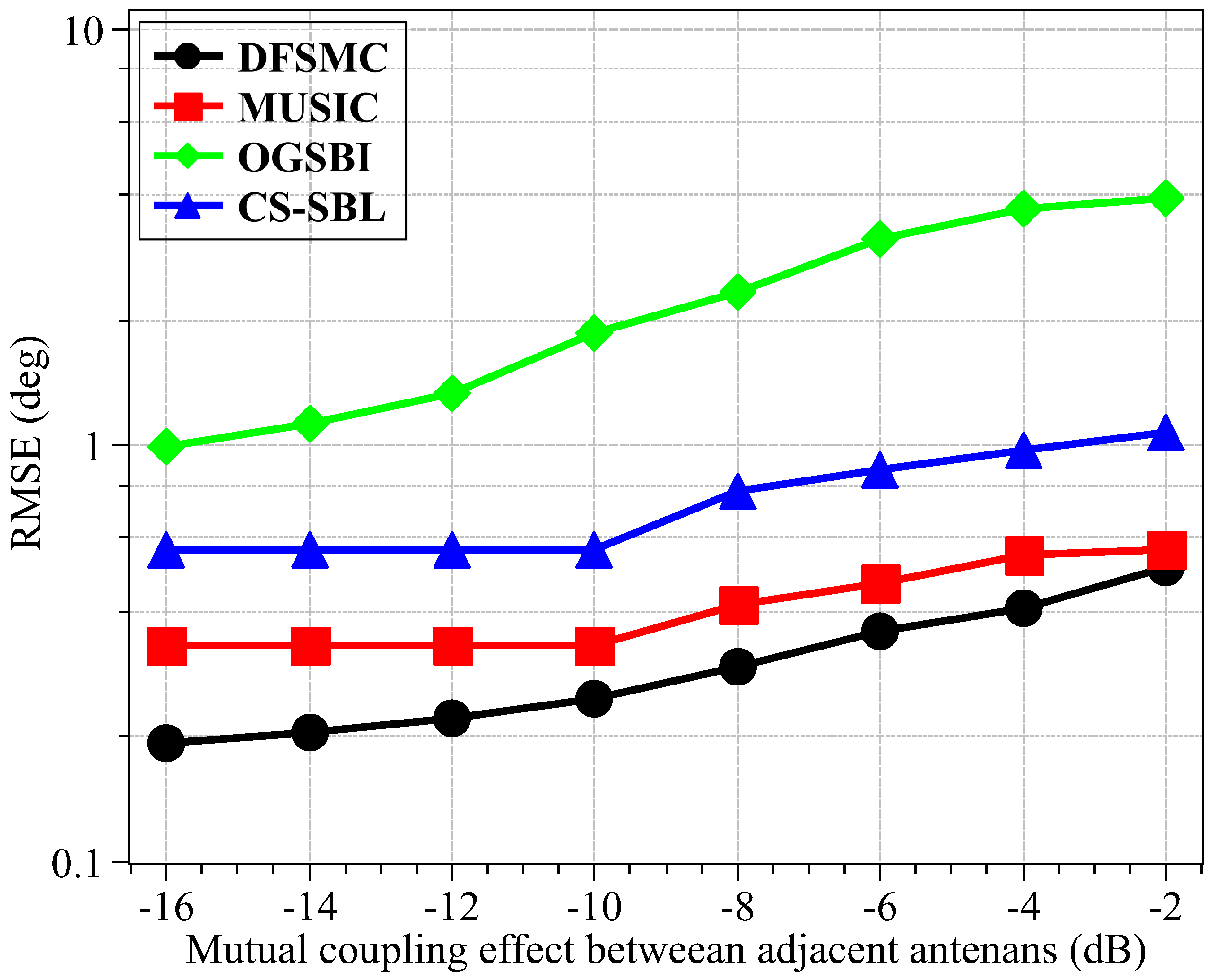
• CS-SBL (The MATLAB code was downloaded at http://people.ee.duke.edu/~lcarin/BCS.html), the Bayesian compressive sensing method proposed in [16].
• OGSBI (The MATLAB code was downloaded at https://sites.google.com/site/zaiyang0248/publication), the off-grid sparse Bayesian inference method proposed in [19].
• MUSIC, the multiple signal classification method [1,2].

With the simulation parameters in

Table 1. Simulation Parameters.

Parameter	Value
The signal-to-noise ratio (SNR)	20 dB
The number of samples M	100
The number of antennas N	20
The number of signals K	3
The space between antennas d	0.5 wavelength
The grid space $\delta$	1°
The direction range	[−60° 60°]
The hyperparameters $b,d,f$	${10}^{-3}$
$N_1$ in Algorithm 1	$N_1={10}^3$
$N_2$ in Algorithm 1	$N_2=300$
$N_3$ in Algorithm 1	$N_3=50$

and the the mutual coupling between adjacent antennas being ${\alpha }_{\mathrm{c}}=-8$ dB, the spatial spectrum is given in Figure 5, where the proposed DFSMC is compared with MUSIC, CS-SBL and OGSBI methods. The estimated directions for $K=3$ signals are given in

Table 2. Estimated directions (${\alpha }_{\mathrm{c}}=-8$ dB).

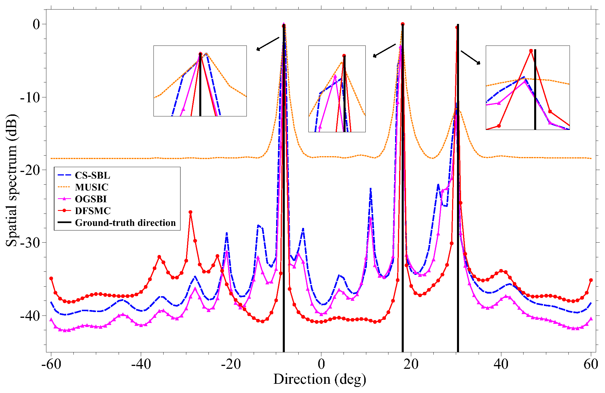
Methods	Signal 1	Signal 2	Signal 3
Ground-truth directions	−8.268°	18.128°	30.428°
OGSBI	−8.267°	17.69°	30.02°
CS-SBL	−8°	18°	30°
MUSIC	−8°	18°	30°
DFSMC	−8.254°	18.13°	30.27°

. Additionally, the iteration processes of DFSMC, CS-SBL, and OGSBI methods are also given in Figure 6. With both the mutual coupling effect and off-grid, the proposed DFSMC method is advantageous in this scenario.

As shown in Figure 6, in the first 300 iterations, DFSMC method only updates the parameters ${\mathbf{\mu }}_m$, ${\mathbf{\Sigma }}_{\mathrm{X}}$ and $\mathbf{\iota }$. Then, during the 301 to 350 iterations, the mutual coupling parameters $\mathit{c}$ and $\mathbf{\vartheta }$ are updated. For the next 50 iterations, the off-grid parameter $\mathbf{\nu }$ is updated. With repeating the 50 iterations to update the mutual coupling parameters and the off-grid parameter, the direction error can be decreased. Moreover, as shown in Figure 6, when only the mutual coupling parameters are updated, the direction estimation performance can be not improved with the correct estimated directions. However, for the next off-grid estimation, the better performance can be achieved with the updated mutual coupling parameters.

The estimated spatial spectrum is shown in Figure 5. It can be seen that the positions of peak spectrum are closer to the ground-truth directions using the DFSMC method than the OGSBI, CS-SBL and MUSIC methods. The corresponding estimated directions are given in Table 2. When we use the following expression to measure the estimation performance

$$\begin{array}{c}\hfill e_1=\sqrt{\frac{1}{K}{\parallel \hat{\mathbf{\theta }}-\mathbf{\theta }\parallel }_2^2},\end{array}$$

(67)

where $\hat{\mathbf{\theta }}$ denotes the estimated directions. Then, the estimation errors (in deg) of DFSMC, OGSBI, CS-SBL and MUSIC methods can be obtained as 0.092°, 0.346°, 0.301° and 0.301°, respectively. Therefore, since the mutual coupling effect is estimated in the proposed DFSMC method, the direction estimation performance is much better than the existing methods including OGSBI, CS-SBL and MUSIC.

When the mutual coupling effect increases from ${\alpha }_{\mathrm{c}}=-8$ dB to ${\alpha }_{\mathrm{c}}=-5$ dB, the corresponding iteration processes and the spatial spectrums of DFSMC, CS-SBL, OGSBI and MUSIC methods are given in Figure 7 and Figure 8. The estimated directions are given in

Table 3. Estimated directions (${\alpha }_{\mathrm{c}}=-5$ dB).

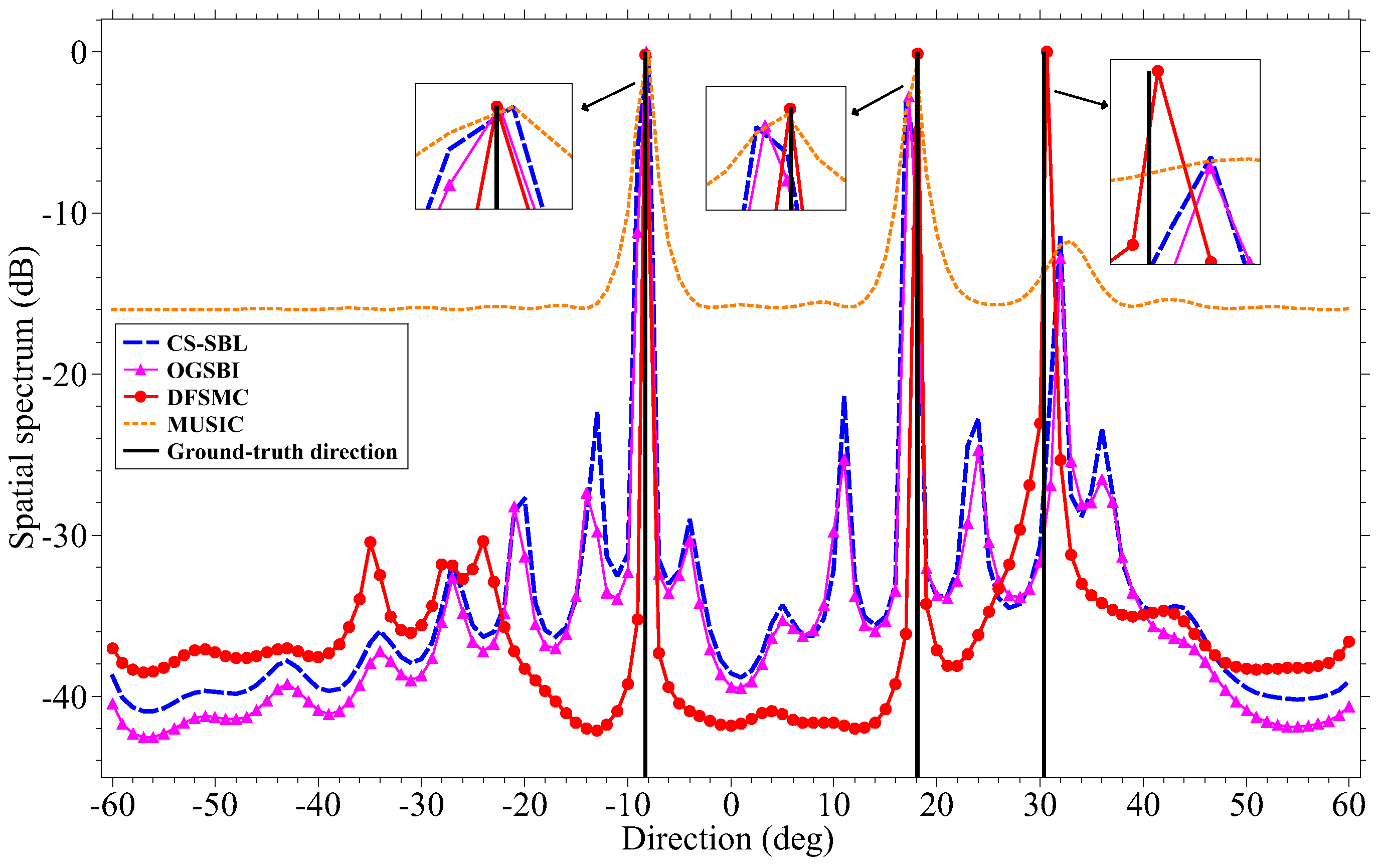
Methods	Signal 1	Signal 2	Signal 3
Ground-truth direction	−8.268°	18.128°	30.428°
OGSBI	−8.222°	17.29°	31.99°
CS-SBL	−8°	17°	32°
MUSIC	−8°	18°	33°
DFSMC	−8.260°	18.11°	30.66°

, and the estimation errors (in deg) of DFSMC, OGSBI, CS-SBL and MUSIC methods can be obtained as 0.134°, 1.024°, 1.128° and 1.495°. Compared with the direction estimation performance in the scenario ${\alpha }_{\mathrm{c}}=-8$ dB, the performance in the scenario ${\alpha }_{\mathrm{c}}=-5$ dB decreases for all the methods, so the mutual coupling effect has a great effect on the direction estimation performance. However, the proposed DFSMC method can also achieve much better performance than existing methods.

With the 100 trails, the direction estimation performance with different SNRs is given in Figure 9, where we use the following root-mean-square error (RMSE) expression to measure the estimation performance

$$\begin{array}{c}\hfill e_2=\sqrt{\frac{1}{KP}{\displaystyle \sum _{p=0}^{P-1}}{\parallel {\hat{\mathbf{\theta }}}_p-{\mathbf{\theta }}_p\parallel }_2^2},\end{array}$$

(68)

where P denote the number of trails, ${\mathbf{\theta }}_p$ denotes the directions in the p-th trail, and ${\hat{\mathbf{\theta }}}_p$ denotes the estimated directions in the p-th trail. As shown in Figure 9, the proposed DFSMC method achieves the best estimation performance when the SNR of received signals is greater than 0 dB. Almost the same estimation performance is achieved by the MUSIC and CS-SBL method. However, with the mutual coupling effect, the direction grids usually cannot be estimated correctly, so the further off-grid optimization in OGSBI cannot improve the estimation performance. Figure 9 indicates that our proposed DFSMC method is very advantageous in the cases when the SNR of received signals is large.

With different mutual coupling effects between antennas, we show the simulation results in Figure 10, where the mutual coupling effect ${\alpha }_{\mathrm{c}}$ between adjacent antennas is from $-16$ dB to $-2$ dB. Since the proposed DFSMC method estimates the mutual coupling vector $\mathit{c}$ iteratively, and DFSMC achieves the best estimation performance among the existing methods including CS-SBL, OGSBI, and MUSIC. It can be seen that with optimizing the off-grid and the mutual coupling vector, the performance of direction estimation can be improved by estimating the sparse signals in the continue domain using the DFSMC method. The computational complexity of the proposed algorithm mainly depends on step 6, step 16 and step 26. The computational complexity of step 6, step 16 and step 26 can be obtained as $\mathcal{O}(M{U}^{2}N+U{N}^2+U^3)$, $\mathcal{O}(U^3+MN{U}^2)$ and $\mathcal{O}(U^3+M{U}^{2}N)$. Therefore, the computational complexity of the proposed algorithm can be obtained as $\mathcal{O}(U^3+M{U}^{2}N+U{N}^2)$. Additionally, with $U\ge N$, the computational complexity can be simplified as $\mathcal{O}\left(MU{N}^2\right)$. The computational complexity of the proposed algorithm has the same order of the SBL-based algorithms, such as the OGSBI algorithm and the SBL algorithm.

5. Conclusions

The direction finding problem with the unknown mutual coupling effect has been investigated in this paper. The novel DFSMC method has been proposed to estimate the directions, the means, and variance of received signals, the mutual coupling vector, the noise variance, and the off-grid vector, et al. iteratively. Additionally, the expressions to estimate the unknown parameters have been theoretically derived using the EM method. Simulation results confirm that the proposed DFSMC method outperforms the existing direction finding methods in the ULA system with the unknown mutual coupling effect. Future work will focus on the extension of the proposed DFSMC method in the scenario with correlated signals.

References

- Schmidt, R.O. Multiple emitter location and signal parameter estimation. IEEE Trans. Antennas Propag. 1986, 34, 276–280. [Google Scholar] [CrossRef]
- Schmidt, R. A Signal Subspace Approach to Multiple Emitter Location Spectrum Estimation. Ph.D. Thesis, Stanford University, Stanford, CA, USA, 1981. [Google Scholar]
- Zoltowski, M.; Kautz, G.; Silverstein, S. Beamspace Root-MUSIC. IEEE Trans. Signal Process. 1993, 41, 344–364. [Google Scholar] [CrossRef]
- Roy, R.; Kailath, T. ESPRIT-estimation of signal parameters via rotational invariance techniques. IEEE Trans. Acoust. Speech Signal Process. 1989, 37, 984–995. [Google Scholar] [CrossRef]
- Pham, G.T.; Loubaton, P.; Vallet, P. Performance analysis of spatial smoothing schemes in the context of large arrays. IEEE Trans. Signal Process. 2016, 64, 160–172. [Google Scholar] [CrossRef]
- Chen, P.; Cao, Z.; Chen, Z.; Yu, C. Sparse DOD/DOA estimation in a bistatic MIMO radar with mutual coupling effect. Electronics 2018, 7, 341. [Google Scholar] [CrossRef]
- Carlin, M.; Rocca, P.; Oliveri, G.; Viani, F.; Massa, A. Directions-of-arrival estimation through Bayesian compressive sensing strategies. IEEE Trans. Antennas Propag. 2013, 61, 3828–3838. [Google Scholar] [CrossRef]
- Chen, P.; Qi, C.; Wu, L.; Wang, X. Estimation of Extended Targets Based on Compressed Sensing in Cognitive Radar System. IEEE Trans.Veh. Technol. 2017, 66, 941–951. [Google Scholar] [CrossRef]
- Yu, Y.; Petropulu, A.P.; Poor, H.V. Measurement matrix design for compressive sensing-based MIMO radar. IEEE Trans. Signal Process. 2011, 59, 5338–5352. [Google Scholar] [CrossRef]
- Carlin, M.; Rocca, P.; Oliveri, G.; Viani, F.; Massa, A. Novel wideband DOA estimation based on sparse Bayesian learning with dirichlet process priors. IEEE Trans. Signal Process. 2016, 64, 275–289. [Google Scholar]
- Chen, P.; Qi, C.; Wu, L. Antenna placement optimisation for compressed sensing-based distributed MIMO radar. IET Radar Sonar Navig. 2017, 11, 285–293. [Google Scholar] [CrossRef]
- Yang, Z.; Xie, L. Enhancing sparsity and resolution via reweighted atomic norm minimization. IEEE Trans. Signal Process. 2016, 64, 995–1006. [Google Scholar] [CrossRef]
- Shen, Q.; Liu, W.; Cui, W.; Wu, S. Underdetermined DOA estimation under the compressive sensing framework: A review. IEEE Access 2016, 4, 8865–8878. [Google Scholar] [CrossRef]
- Yang, Z.; Xie, L. Exact joint sparse frequency recovery via optimization methods. IEEE Trans. Signal Process. 2016, 64, 5145–5157. [Google Scholar] [CrossRef]
- Tipping, M.E. Sparse Bayesian Learning and the Relevance Vector Machine. J. Mach. Learn. Res. 2001, 1, 211–244. [Google Scholar]
- Ji, S.; Xue, Y.; Carin, L. Bayesian compressive sensing. IEEE Trans. Signal Process. 2008, 56, 2346–2356. [Google Scholar] [CrossRef]
- Wu, X.; Zhu, W.; Yan, J. Direction of arrival estimation for off-grid signals based on sparse Bayesian learning. IEEE Sens. J. 2016, 16, 2004–2016. [Google Scholar] [CrossRef]
- Chen, P.; Zheng, L.; Wang, X.; Li, H.; Wu, L. Moving target detection using colocated MIMO radar on multiple distributed moving platforms. IEEE Trans. Signal Process. 2017, 65, 4670–4683. [Google Scholar] [CrossRef]
- Yang, Z.; Lihua, X.; Cishen, Z. Off-grid direction of arrival estimation using sparse Bayesian inference. IEEE Trans. Signal Process. 2013, 61, 38–43. [Google Scholar] [CrossRef]
- Dai, J.; Bao, X.; Xu, W.; Chang, C. Root sparse Bayesian learning for off-grid DOA estimation. IEEE Signal Process. Lett. 2017, 24, 46–50. [Google Scholar] [CrossRef]
- Wang, Q.; Zhao, Z.; Chen, Z.; Nie, Z. Grid evolution method for DOA estimation. IEEE Trans. Signal Process. 2018, 66, 2374–2383. [Google Scholar] [CrossRef]
- Zamani, H.; Zayyani, H.; Marvasti, F. An iterative dictionary learning-based algorithm for DOA estimation. IEEE Commun. Lett. 2016, 20, 1784–1787. [Google Scholar] [CrossRef]
- Clerckx, B.; Craeye, C.; Vanhoenacker-Janvier, D.; Oestges, C. Impact of Antenna Coupling on 2 × 2 MIMO Communications. IEEE Trans. Veh. Technol. 2007, 56, 1009–1018. [Google Scholar] [CrossRef]
- Zheng, Z.; Zhang, J.; Zhang, J. Joint DOD and DOA estimation of bistatic MIMO radar in the presence of unknown mutual coupling. Signal Process. 2012, 92, 3039–3048. [Google Scholar] [CrossRef]
- Rocca, P.; Hannan, M.A.; Salucci, M.; Massa, A. Single-snapshot DoA estimation in array antennas with mutual coupling through a multiscaling BCS strategy. IEEE Trans. Antennas Propag. 2017, 65, 3203–3213. [Google Scholar] [CrossRef]
- Liu, J.; Zhang, Y.; Lu, Y.; Ren, S.; Cao, S. Augmented nested arrays with enhanced DOF and reduced mutual coupling. IEEE Trans. Signal Process. 2017, 65, 5549–5563. [Google Scholar] [CrossRef]
- Hawes, M.; Mihaylova, L.; Septer, F.; Godsill, S. Bayesian compressive sensing approaches for direction of arrival estimation with mutual coupling effects. IEEE Trans. Antennas Propag. 2017, 65, 1357–1367. [Google Scholar] [CrossRef]
- Basikolo, T.; Ichige, K.; Arai, H. A novel mutual coupling compensation method for underdetermined direction of arrival estimation in nested sparse circular arrays. IEEE Trans. Antennas Propag. 2018, 66, 909–917. [Google Scholar] [CrossRef]
- Zhang, C.; Huang, H.; Liao, B. Direction finding in MIMO radar with unknown mutual coupling. IEEE Access 2017, 5, 4439–4447. [Google Scholar] [CrossRef]
- Liao, B.; Zhang, Z.G.; Chan, S.C. DOA estimation and tracking of ULAs with mutual coupling. IEEE Trans. Aerosp. Electron. Syst. 2012, 48, 891–905. [Google Scholar] [CrossRef]
- Termos, A.; Hochwald, B.M. Capacity benefits of antenna coupling. In Proceedings of the 2016 Information Theory and Applications (ITA), La Jolla, CA, USA, 31 January–5 February 2016; pp. 1–5. [Google Scholar]
- Liu, X.; Liao, G. Direction finding and mutual coupling estimation for bistatic MIMO radar. Signal Process 2012, 92, 517–522. [Google Scholar] [CrossRef]