Abstract
Renewable energy sources, on one hand, are environmentally friendly, but on the other, they suffer from volatility in power generation, which endangers power-grid stability. A viable solution to circumvent the intermittent behavior of renewables is the usage of energy-storage systems. In this paper, we study the energy management of a proof-of-concept system consisting of solar panels, energy-storage systems, a power grid, and household loads. Using neural networks, we identify the most relevant parameters impacting the power generation of solar panels, and then train the corresponding network to derive forecasts. We also go one step further, and propose a heuristics-based energy-management policy for the purpose of reducing curtailments. We show that our proposed policy outperforms the naive policy by 8%, which does not consider any power-generation forecasts.
1. Introduction
In recent years, the inclusion of Renewable Energy Sources (RES), such as photovoltaic systems and windmills, into our cities has been pervasive. Furthermore, the capacity of RES installed all over the globe has been rising with increasing speed [1], driven by the need to tackle climate change, which necessitates, more than ever, the usage of environmentally friendly energy sources. Consequently, a great deal of attention has been drawn toward the problems and limitations involved with power generation from RES. The major drawback of those renewable sources is their intermittent generation behavior (e.g., mostly dependent on weather conditions). This volatile nature of RES causes a mismatch between power generation and demand, which, in turn, endangers the grid’s stability [2].
To mitigate this problem, new solutions have lately been suggested to optimize the production, consumption, and storage of electricity. To this end, energy-storage systems (ESS) [3] have been proposed to operate in conjunction with RES, so that the full potential of those sources can be exploited. Instead of curtailing generation during peak periods, energy can be stored and later be used whenever needed. Nevertheless, most installations still have to curtail generation when storage capacity is full, which necessitates the need for optimized storage management.
Given the importance of the topic, in this paper we study the energy management of systems that assume (1) solar panels as producer, (2) energy-storage systems and power grid as prosumers, and (3) a local household load as consumer. Note that such systems are becoming increasingly common in real-life use cases. To this end, as proof of concept, we consider and study one of the real-world products of Fenecon GmbH (https://fenecon.de/en_US/), which is a company in southern Germany specialized in photovoltaic and energy-storage systems.
The main objective of this work is to provide optimized energy management to the aforementioned systems by reducing the amount of curtailed electricity due to regulation laws; there is a law in Germany that constrains the maximum amount of power that can be fed back into the grid generated by small installations. If the amount of energy to be generated in the near future is known (through forecasts) ahead of time, enough storage capacity can be reserved, and generated energy can be fed into the grid in a constant manner that does not endanger grid’s stability.
To achieve this, we derived power-generation forecasts using neural-network methodology. We gathered three different data sources (e.g., generation, irradiation, and weather) and identified the most influential parameters on power generation. Furthermore, we used the identified parameters to train three different neural networks and choose the most suitable one based on the accuracy of the obtained results. We went one step further and proposed two policies: “Naive” and “Loss Avoidance”. Unlike the former, the latter is a heuristics-based optimized energy-management policy that is empowered by photovoltaic (PV) power-generation forecasts. Moreover, we set up simulations by considering both “Naive” and “Loss Avoidance” policies, and we show that the latter, thanks to the incorporated power-generation forecasts, provides significant improvements in preventing the curtailment of power generation.
The rest of this paper is organized in the following manner: In Section 2, we describe terms relevant to the considered system as well as the methodology related to the neural network. Section 3 highlights similar contributions in the literature. Section 4 provides the derivation of power-generation forecasts using neural-network methodology. In Section 5, we present our proposed optimized energy-management policy and compare it against “Naive”, which does not incorporate any PV power-generation forecasts. The paper is concluded in Section 6.
2. Preliminaries
In this section, we give definitions and explanations to the terms that are used in the rest of this paper. In Section 2.1, we present generic technical terms related to the considered system, and then describe methodology-related matters in Section 2.2.
2.1. Technical Terms
Figure 1 shows a high-level overview of the different parts involved in the considered system, which are described next.
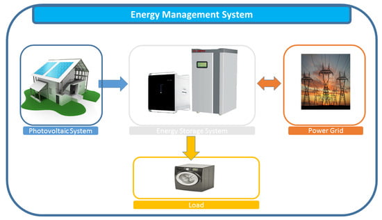
Figure 1.
A sample system consisting of photovoltaics (PV), an energy-storage system (ESS), power grid, and household load, which is managed by an EMS.
2.1.1. Photovoltaic System
Solar panels generate green and clean energy and, upon establishment of a closed electric circuit, direct current (DC) becomes available. To use it for standard electric devices or feed it into the power grid, it has to be converted to alternating current (AC) using an inverter. A photovoltaic system usually consists of several to hundreds of solar panels, being quantified by the nominal output power in Watt (W) during Standard Test Conditions (STC). The unit is formally referred to as “watt-peak” (Wp) or, more commonly, “kilowatt-peak” (kWp).
2.1.2. Energy-Storage System
With the growing need for nontraditional (e.g., fossil-based) power-generating sources, it becomes vital to overcome the fluctuating and volatile nature of renewables. The idea is to keep excessive generated power, which cannot be immediately consumed, in storage systems for later usage. The technologies are categorized according to their storage period, from short-term (e.g., flywheels, supercapacitors, or batteries), to seasonal (e.g., power-to-gas, pumped-storage hydroelectricity), and others.
While many different approaches for storing energy have been developed, only few of them currently fulfil the requirements for small decentralized installations with minimum maintenance and reasonable economic efficiency. One of those few approaches is the lithium-ion battery technology.
2.1.3. Power Grid
Generally, it is expected that any household, industrial site, or other consumer are directly connected to an Energy Supplier (ES) through the grid infrastructure provided by Distributed System Operators (DSOs). In most countries, this power grid is constantly available with high reliability. Furthermore, electricity can be purchased for a static price that is usually fixed over a long period of time, like a month or a year.
Table 1 gives the electricity prices (in euro cents per kilowatt-hour) of households in Germany (https://www.statista.com/statistics/418078/electricity-prices-for-households-in-germany/). Based on a survey conducted by Eurostat (http://ec.europa.eu/eurostat/statistics-explained/index.php/Electricity_price_statistics), it is shown that electricity prices for households in Germany are above average European prices. As electricity-production costs increasingly differ throughout the day and year because of the ongoing transition to renewable sources, flexible tariff models with varying electricity prices have been put in place [4].

Table 1.
Electricity prices for households in Germany from 2014 to 2017, semiannually (in euro cents per kilowatt-hour).
In a setup (that the current paper considers) with photovoltaic and energy-storage systems, power can be drawn from the grid only when local and decentralized electricity generation is not sufficient to satisfy the needs of the loads. In case there is an excess (e.g., the needs of the ESS and loads are satisfied) of electricity generation, the rest can be fed back to the power grid. In order to speed up the increase of solar energy, different feed-in tariffs [5] were proposed in the form of subsidies in major European countries with certain constraints. For instance, enacted by the German Renewable Energy Act 2014 (EEG 2014), the feed-in for small systems (e.g., under 50 kWp) in Germany is restricted to 50% of the installed panels’ peak power generation. It is worthwhile to note that, in this paper, we consider this feed-in constraint in our analysis.
2.1.4. Energy-Management Systems
Technically, ESSs are located between the energy-production units (e.g., photovoltaic systems), the power grid, and the electric loads, so that the energy flow is accordingly managed by the system. At any point in time, the system combines an energy mix generated from three different sources: (1) the PV system, (2) the energy-storage system, and (3) the power grid. This necessitates an energy-management system (EMS) that is able to optimize generation from aforementioned available electricity sources. This optimization is based on a set of rules that specify a prioritization list in choosing different energy sources.
2.2. Methodological Terms
In this section, we present basic background information about Artificial Neural Networks (ANN) and three different types of networks relevant to our study. Note that a detailed description can be found in the literature and hence is out of the scope of this paper.
2.2.1. Artificial Neural Networks (ANN)
An ANN is a methodology based on Machine Learning that was first proposed back in the 1950s. It was inspired by the manner in which the human brain processes and learns information through neurons. With the technological advances of computing systems, as well as the increasing importance that data analysis has received in the last decade in all disciplines, Neural Networks have been gaining increasing attention.
The terminology of ‘perceptron’ mathematically denotes the concept of a neuron in ANNs. It consists of (1) a set of inputs where each such value has a specific weight that leads to amplifying or degrading the corresponding value, (2) an activation function f where the sum of all the weighted values is passed, and (3) an output y generated from this activation function:
Equation (1) demonstrates the way the output of the perceptron is calculated by using forward propagation. An important characteristic of the perceptron is that it is able to learn and hence adjust the weights from the dataset in a backward fashion. To this end, a back-propagation algorithm [6] was proposed that calculates error E as the difference between calculated output y of the perceptron and ideal target output t:
By calculating the error using Equation (2), it could be then possible to adjust the perceptron’s weights by a defined learning rate of r:
As a result, through several iterations of the algorithm, the perceptron’s output y comes closer to the ideal targeted output t.
Based on the basic concept of the perceptron, a Multilayer Perceptron (MLP) network was proposed to construct an architecture that consists of input, hidden, and output layers. In this architecture, the calculated output y of each perceptron is used to serve as an input to the perceptrons on the next layer. By applying the forward- and back-propagation algorithms on enough dataset pairs with input and ideal output vectors, the MLP network can learn sophisticated nonlinear functions. Next, we describe three types of MLP-based ANNs relevant to our study. Note that the choice of those networks are made due to the usage of the Encog (https://www.heatonresearch.com/encog/) framework in Section 4.3, which is an open-source library for machine learning that supports implementation for those networks available in programming language Java. The usage of Java is required, as the energy-management system OpenEMS (https://github.com/OpenEMS/openems) of Fenecon GmbH is developed in this programming language. Moreover, OpenEMS was the main management system for our considered proof-of-concept system.
2.2.1.1. Feed-Forward Neural Network (FFNN)
FFNN is a very basic type of ANN where data only flow in the direction from the input to the hidden and then to the output layers. Furthermore, such type of network contains no loops or cycles such that the output of one layer is fed to another layer. The network type is known to have a slow learning speed due to the computationally expensive learning process based on gradient descent and the iterative tuning of weights.
2.2.1.2. Radial Basis Function Network (RBFN)
RBFN has an input, output, and normally one hidden layer. The hidden layer contains all the radial basis functions (e.g., normal distribution) having different parameters. Thus the output of the network is calculated as a linear combination (e.g., weighted sum) of the outputs from radial basis functions of the hidden layer. The learning process of an RBFN has two stages: At first, the center and width of the radial basis functions are set. The center can be randomly chosen from the dataset or the data can be clustered (e.g., k-means clustering) since the center of a cluster is the point with the lowest aggregated distance to all points contained by this cluster. In the second step, the weights assigned to the connections are modified based on gradient descent and iterative tuning. Here again, the back-propagation technique can be used to improve the learning rate.
2.2.1.3. NeuroEvolution of Augmenting Topologies (NEAT)
NEAT is a genetic algorithm to evolve ANNs by creating a set of randomly initialized networks. Those networks are evaluated in terms of how precise their outputs are. Then, the iterating process of evolution is performed until a network of desired quality is derived.
When applying the concept of genetic evolution to the construction of neural networks, the nodes and their connections form the genome. The overall process is very similar to and inspired by breeding: Phenotypes with desired attributes (e.g., high precision in classification, regression, etc.) are cross-bred to enhance them further. In the context of ANNs, cross-breeding is achieved by the recombination of the selected networks’ nodes and connections with the assigned weights.
The evolutionary optimization process of NEAT tends to be faster than the conventional learning techniques of FFNN and RBFN. Furthermore, the network topology of FFNN and RBFN is chosen by a human experimenter, and effective connection weight values are learned through a training process, as explained previously. This yields a situation whereby a trial-and-error process may be necessary in order to determine an appropriate topology. NEAT is an example of a topology and weight-evolving ANN that attempts to simultaneously learn weight values and an appropriate topology for a neural network.
2.2.2. Statistical Methods
In this section, we present methods used to compare how close (e.g., to calculate accuracy) two random variables are. Those error-measuring methods are used in Section 4.3.1 (see Table 5) in order to compare the different ANNs (e.g., FFNN, RBFN, and NEAT) used to forecast PV power generation. As every respective measure indicates a certain quality of the derived forecasts, each of them is used to demonstrate a certain characteristic of the corresponding forecasts.
2.2.2.1. Mean Absolute Error (MAE)
MAE is the average of the distance between predicted and observed values and is given by:
For each observation, the distance between observed and predicted value is added and the sum is then divided by the number of observations to obtain the average per observation. Because errors are not modified, the MAE is a good choice to measure the general accuracy of a prediction.
2.2.2.2. Mean Square Error (MSE)
MSE is the average of the squared distance between predicted and observed values and is given by:
It measures the quality of the estimator and quantifies the prediction’s average spreading around the actual value.
2.2.2.3. Root Mean Square Error (RMSE)
RMSE is the sample standard deviation of the differences between predicted and observed values and is given by:
It is the square root of the Mean Square Error (MSE). The RMSE, like the MSE is highly affected by large errors since they are squared before taking the average. This makes the measure adequate to qualify predictions featuring single high errors.
2.2.3. Pearson’s Correlation
Pearson’s correlation [7] is a measure for the linear correlation of two random variables, X and Y. It is calculated as the ratio of the covariance of those two variables to the product of their standard deviations:
It ranges between −1, representing a total negative linear correlation, and 1, which is total positive linear correlation. A zero value indicates no correlation at all. We use Pearson’s correlation in Section 4.1 (as the first step of our proposed methodology) to identify among the set of several considered parameters the most correlated ones impacting power generation of PV solar panels.
3. Related Work
Since the contributions in this paper are twofold, we introduce in this section the works in the literature from those two perspectives.
3.1. PV Power-Generation Forecasts
Several recent contributions investigate the possibilities in forecasting PV power generation. Stochastic models can be used for short- and long-term predictions. Ramakrishna et al. [8] introduced a regime-switching approach by utilizing different models for different weather conditions to improve overall precision. Ghiassi–Farrokhfal et al. [9] combined different time spans, where the basic interday irradiance was modeled in larger time slots to represent the basic trend with a peak at midday. Another model was then created to map the momentary but intense fluctuations in a time span of up to ten minutes. Both models were then combined to create a generic one that outperforms standard predictors.
Besides analytical models, research was conducted on the possibilities of machine-learning techniques to predict photovoltaic generation. Shi et al. [10] demonstrated the usage of Support Vector Machines as a field of machine learning to predict power output based on weather classification. By dividing the test data upon the weather condition prevailing each day (i.e., sunny or rainy), four different models were derived. Each of those performs accurately on its specialized case. The authors were able to generate forecasts with a mean relative error of 8.64% over all the data. Yona et al. [11] showed that the usage of ANNs is eligible for the prediction of solar irradiation. The authors compared the performance of different types of ANNs (see Section 2.2.1) against each other and discussed the varying precision during different months. The types under investigation were FFNN (see Section 2.2.1.1) and RBFN (see Section 2.2.1.2). In Reference [12], the authors proposed a methodology for short-term (e.g., 15 min) forecasting of global horizontal irradiance (GHI) using a nonlinear autoregressive neural network. Simulations were used in order to predict the power production of solar panels in a short time.
The aforementioned approaches first forecast irradiation values, and then use them to further calculate the power generation of PVs. What is lacking so far is an in-depth analysis of the different factors impacting the power generation of solar panels. Hence, in our approach we propose a new methodology, and first carry out a Pearson’s correlation on all the attributes of the gathered data sources. Based on the results, we identified the most relevant parameters to power generation. Those identified parameters were then used to train three different neural networks: FFNN, RBFN, and NEAT. Furthermore, we evaluated the accuracy of the power-generation forecasts of each of those types. The added value of our contribution to the above-mentioned approaches is that our proposed methodology is generic enough that can be applied to estimate the power generation of PVs of different sizes and geographic locations.
3.2. Energy-Management Optimization
In Reference [13], the authors investigated systems consisting of PV panels and energy-storage systems (e.g., batteries), and analyzed the effect of energy policies on the adoption of such systems in the region of Ontario (Canada). The authors then extended their work in Reference [14] and included the state of Bavaria (Germany) in their analysis. The results show that there exist different adoption behaviors in those countries due to the policies and incentives of the respective jurisdictions. In Reference [15], the authors studied the problem of optimally sizing solar photovoltaic and energy-storage systems. They evaluated the robustness and complexity of computations for their system sizing decisions in a realistic setting.
Apart from those studies, a great deal of attention was dedicated to optimizing the usage of PV–ESS systems from a price perspective. To this end, in Reference [16] the authors studied the optimal operation of a consumer-based ESS in combination with intermittent renewable generation of PVs, where time-varying electricity prices and different types of AC/DC household loads were considered. Maximizing the long-term expected payoff of consumer-based systems consisting of ESS and PVs was studied in Reference [17]. The authors showed that the consumer’s maximum expected payoff is piecewise linear in the storage level for the case of inelastic loads. Furthermore, in case the price and load demand are both deterministic, the authors established the equivalence between the optimal storage operation problem and a minimum cost flow problem. Using linear programming, the authors in Reference [18] proposed an optimal operation of ESS by assuming that the household load follows a Gaussian distribution, and power generation of PVs has a binomial distribution.
The main differentiator of our work from the above-mentioned approaches is the fact that we consider optimization policies that tackle systems consisting of PV solar panels, ESSs, power grids, and household loads. Note that such a type of systems is increasingly pervading in our cities as real-life products that were previously not possible due to the high prices of ESSs. Furthermore, unlike the others, in our considered system it is possible to feed power back into the grid by taking into account constraints on this amount due to jurisdiction. In order to reduce PV power-generation curtailment, which has not been considered as an optimization objective in the aforementioned scientific contributions, we propose a heuristics-based policy. To the best of our knowledge, this is the first paper that considers reduction of PV power-generation curtailment. To achieve this, we incorporate the PV power-generation estimation model into a PoC system of Fenecon GmbH.
4. Forecasting of Power Generation
For any EMS to take optimal decisions on when to charge/discharge the ESS and feed in/draw power to/from the grid, it is of utmost importance that such an EMS be equipped with a forecasting module. The objective of such a module is to estimate the amount of power that can be generated from the corresponding installed solar panels. The generated forecasts can be later used for day-ahead planning purposes.
In this section, we first present our proposed methodology to identify the relevant parameters impacting on the power generation forecasts of solar panels. Furthermore, based on the derived analysis, we then evaluate the accuracy of those forecasts by considering three different types of networks, namely FFNN, RBFN, and NEAT.
4.1. Proposed Methodology
In order to identify the most relevant parameters impacting on the power generation of solar panels, an analysis was carried out on a consolidated dataset by applying the following methodology:
- Information of the consolidated dataset fetched from three different data sources (PV power generation, weather, and irradiation) is considered.
- The set of correlated and causally related attributes are identified using Pearson’s correlation on all the attributes of the consolidated dataset of Step 1.
- The corresponding network under study is trained using three different neural networks while altering attribute sets to identify those with the highest impact on prediction precision. Those types are compared against each other in order to identify the most accurate solution.
4.2. Correlation Analysis
In this section, we present the results of the analysis carried out on the consolidated dataset by applying the methodology of Section 4.1. We started (Step 2) with Pearson’s correlation (see Section 2.2.3) and then, based on the results of this correlation, analysis was performed using a neural network (Step 3).
Table 2 illustrates the corresponding Pearson’s correlation of the different considered attributes of the consolidated dataset given in percent. Note that green and red cells denote positive and negative correlations, respectively. When inspecting the table, one must remember that correlation does not imply causation (e.g., indicates that one event is the result of the occurrence of the other event). For instance, the relatively high correlation between the clear-sky GHI (e.g., CSG) on the one hand and the temperature (e.g., TP) on the other hand is a good example for that. The clear-sky GHI is dependent on the sun’s current activity in terms of insolation and the angle between the site of observation and the sun.
Table 2.
Pearson’s correlation of different attributes over the whole observation time presented in percent. For the symbols and their definition, see Table 3.
Still in comparison with aforementioned clarification, the correlation of the GHI with the cloud cover (e.g., CC) might show causation. The high correlation between clear-sky GHI and cloud cover is argued to be random, but the difference to the correlation between GHI and cloud cover can be interpreted as causal, where the rationale is explained next. GHI is the product of the clear-sky GHI and the clear-sky index, which indicates how little the insolation reaching the atmosphere is absorbed on the way to ground level. This means GHI and cloud cover, which is the percentage of the sky covered, must be indirect proportional effects and therefore have a lower Pearson’s correlation than the random one between clear-sky GHI and cloud cover.
There is also a causal explanation for the high correlation between temperature and GHI, and clear-sky GHI, respectively. Fluctuation in the irradiation reaching the atmosphere (e.g., respectively the ground plane) is the main reason for deviation in temperature. Meteorologic phenomena like wind and cloud cover are a direct consequence of regional temperature differences which weaken the correlation but not the causation. Therefore, the irradiation is a direct source of increase in temperature.
Temperature, on one hand, and wind speed (WS), respectively, wind gust on the other hand, are negatively correlated since wind is not a consequence of local temperature but rather the temperature difference between two arbitrary regions where neither of those regions is the site of observation. In fact, wind in the region of the considered site is often caused by temperature differences between the Atlantic Ocean and the Eurasian land mass. This also explains the correlation of temperature and cloud cover being close to zero as well. Cloud cover is not caused by local temperature, but depending on whether the wind moves during cloudy or clear weather conditions towards the considered site. Those attributes have a causal relation between each other, but it is a far more complex system than a linear correlation.
Humidity (HM) could be seen as combination of effects like cloud cover and precipitation intensity (PI) and its probability (PP). Therefore, the low correlation between cloud cover and humidity is unexpected at first sight, but can be explained by weather conditions of dry cloudy days as well as humid mornings and evenings with clear sky. The negative correlation between humidity and insolation (DHI and GHI), with the absolute values of 0.46 and 0.63, might indicate a meaningful relation.
At a certain level, a higher temperature causes higher panel efficiency and, therefore, higher power generation (MP) for the same amount of insolation. Nevertheless, the high correlation of temperature and power generation is mostly caused by the correlation of temperature and insolation, and rather unlikely to be the consequence of the minor increase in panel efficiency. We know that the amount of generated power is directly dependent on the irradiate. Hence, as expected, correlation is highest between the different types of irradiation (i.e. CSG, CSD, GHI, DHI) and power generation.
Visibility (VS) and cloud cover both indicate sky clearness and therefore influence the amount of irradiation reaching the ground plane. Their effect on power generation is already implicitly taken into account when using the GHI instead of the clear-sky GHI. The differences in correlation between those attributes (i.e., VS and CC) with respect to GHI and clear-sky GHI, respectively, confirm this. The negative correlation of those attributes among each other illustrates that irradiation is the most important influencing factor.
To conclude, from the Pearson’s correlation analysis presented in this section, it can be clearly noted that both GHI and temperature can be used as useful parameters in estimating the power generation of the solar panels. This fact is illustrated in Figure 2, Figure 3 and Figure 4 that capture power generation, global horizontal irradiance, as well as ambient temperature, respectively, during the period between 1 May 2017 and 30 April 2018 such that the X-axis of those figures denotes the hour of the day scaled between 00:00 and 23:00 on an hourly basis. Furthermore, Figure 5 demonstrates the average yearly power generation and irradiation. It can be seen from those figures that peak power generation happens at 13:00, which coincides with the corresponding peak values of irradiation and temperature. It is important to note that, although the gathered data sources are from the southern region of Bavaria (Germany), the derived conclusions of this section are generic enough to be applicable to any region having similar characteristics as the one considered in this paper.
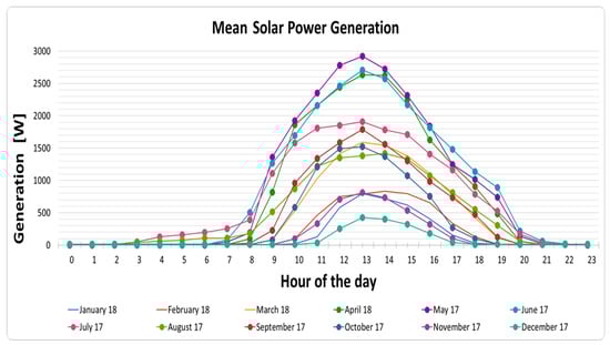
Figure 2.
Mean power generation on a monthly basis given in 24 hours per day.
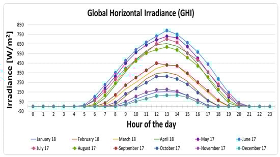
Figure 3.
Global horizontal irradiation on a monthly basis given in 24 hours per day.
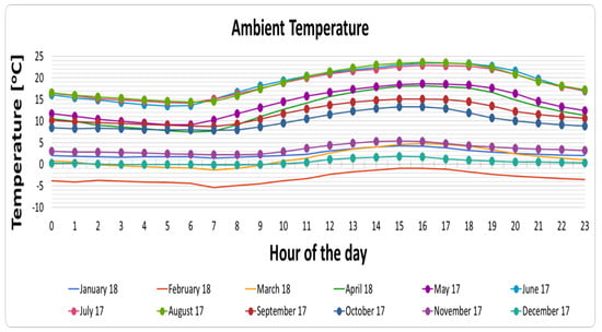
Figure 4.
Ambient temperature on a monthly basis given in 24 hours per day.
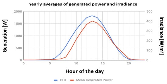
Figure 5.
Generated power and irradiation on a yearly basis given in 24 hours per day.
Next, we present the different neural-network types that were used in order to train the corresponding networks by having both GHI and temperature as input parameters.
4.3. Neural-Network Analysis
In this section, analysis is carried out by taking into account three different neural networks. First, details on construction and training are given, and then the results of the corresponding evaluation are presented.
4.3.1. Adopted Training Technique
In our initial tests, in addition to the regression technique, we also considered both the classification approach and the usage of a time series. As the latter two techniques did not produce results comparable in precision with respect to the regression one, forecast of PV power generation was performed by means of regression.
Based on the analysis carried out in Section 4.2, the chosen attributes were the GHI and temperature, as those did not only have the highest correlation with respect to PV power generation, but also had causal relation (see Section 4.2). Experiments with additional attributes showed no improvements in forecasts, which leads to the conclusion that (1) some correlations are random, and (2) GHI implicitly contains causally related features like cloud cover (an extensive analysis of the consolidated dataset can be found in Section 4.2).
Table 4 lists the RMSE for training and validation of the different types of neural networks. These were trained by performing fivefold cross-validations using 70% of the data as the training set. Next, a discussion about those results is given.
Table 4.
Results of training by taking into account GHI and temperature and considering three different neural-network methods.
4.3.2. Evaluation and Results
For this evaluation, the error computation methods of MAE, MSE, and RMSE (see Section 2.2.2) were used. Table 4 illustrates the results of the training phase that were realized on a computer with an i7-800K processor, 4.4GHz, and 32GB of RAM. While comparing the results, it can be seen that the performance of FFNN was worse when looking at the cross-validation score as well as training and validation errors. This is due to a relatively low learning speed and the limited amount of available training data. The NEAT network needed the longest training in terms of elapsed time. Only during this training, CPU utilization rate was above 95% on all six cores. This is the consequence of the exhaustive trial-and-error principle of the underlying genetic algorithm. The cross-validation score and errors in contrary are best. This suggests the usage of the NEAT network since training is done on a separate machine and is therefore not limited to the hardware the EMS controller is running on.
The resulting predictions were checked against each other by comparing previously introduced error measures (e.g., MAE, MSE, RMSE), quantifying the deviations between each forecast and the actual generation. Table 5 shows the results by taking into account the aforementioned three error measures, as well as neural-network types. The usage of RBFN resulted in the highest MAE, which indicates, on average, wider deviation from the actual values. Furthermore, the highest RMSE was caused by having outliers significantly deviating from the average. Again, the NEAT network outperformed its competitors. Consequently, the results obtained in this section confirm the suitability and advantage of the NEAT method over the other two, namely, FFNN and RBFN.
Table 5.
Error measures of predictions by considering three different neural methods.
5. Heuristics-Based Optimization
In this section, we introduce two policies applied to the system described in Section 2.1: a naive and heuristics-based optimization empowered by PV forecasts. Thanks to the forecasting module of Section 4, we show that the proposed optimized policy has improvements in respect to the naive one that has a myopic view (e.g., no forecasts).
As proof-of-concept, we considered the production system of Fenecon GmbH by studying the following technical characteristics and constraints:
- Photovoltaic System: The system under study is equipped with an array of 36 panels, each generating 280 Wp with a total overall peak generation of 10.08 kWp.
- Energy-Storage System: The system under study is equipped with a BYD PRO Hybrid 9–10 energy-storage system. It provides a usable storage capacity of 9 kWh with a guaranteed number of 6000 cycles until a remaining capacity of 80%. This equates to an average of 300 cycles per year for an expected life span of 20 years. The ESS degree of efficiency for charging and discharging taken from the data sheet is 93%.
- Feed-in Grid: In this work, we consider the feed-in maximum power constraint to be 50% of the installed panels’ peak power generation (e.g., 5 kWp).
5.1. Considered Policies
5.1.1. Naive Policy
This policy takes decisions as follows: If generation of the photovoltaic system exceeds the power needs of the local loads, then use this excess of electricity to charge the energy-storage system with a maximum charging rate as long as the system has enough charging capacity. While charging the ESS, there is still excess of electricity; then, feed the remaining back to the power grid. In case there is a deficit of generation from the photovoltaic system, the ESS is used to satisfy the needs of the load as long as it has enough stored capacity. Electricity from the grid is used to satisfy the needs of the load whenever the electricity provided by the ESS is not enough (residual energy), or the ESS has no storage capacity. The corresponding generation needs to be curtailed any time that the maximum feed-in constraint of the power grid is exceeded. Algorithm 1 gives the different steps of the “Naive” policy.
| Algorithm 1: Naive Policy |
 |
5.1.2. Loss Avoidance
Is our proposed heuristics-based optimized policy to minimize curtailment that takes decisions in the following manner: Since the maximum feed-in to the power grid is limited, there can occur situations where the generation exceeds this limit. If the ESS is already full during this state, the generation has to be curtailed. If the system could predict such situations, it could plan enough storage capacity for the generation such that this energy would have been otherwise curtailed. Hence, the idea is to feed energy into the grid instead of charging the ESS at an earlier time to prepare the need for later charging. Consequently, to achieve this, the corresponding policy consists of two different phases: Planning and Optimization. In the Planning phase, for each timeslot of the corresponding day, first a coarse plan on how to use the available energy is generated, similar to the one applied by Algorithm 1. However, the main differentiator here is the generation forecasts (see Section 4) that help to predict the power generation of the photovoltaic system in a day-ahead fashion. In case more energy is available, then this can be used to charge the ESS and feed into the grid so that the remaining surplus is remembered. In the Optimization phase, the remembered surplus is handled. The algorithm iterates the timeslots in a backward direction to identify a candidate slot where more energy can be fed into the grid to clear storage capacity for the surplus later on. The amount of charge delayed to absorb the surplus, at least partially, is limited by the intermediate timeslots. The delay of charge must not lead to the depletion of the ESS. During the course of the day, the ESS is charged as planned, the remaining available energy is fed into the grid and discrepancy between planning and real execution is logged. Algorithm 2 gives the different steps of the “Loss Avoidance” policy.
| Algorithm 2: Loss Avoidance Policy |
 |
It is worthwhile to mention that computation of possible charge reduction on line 25 is carried out in the following manner: For candidate timeslot c and given timeslot t such that there is potential excess of energy with curtailment needed:
- Find the maximum amount of charge reduction dependant on the intermediate timeslots: For each intermediate timeslot i where , obtain the amount of energy drawable from ESS, then take the minimum of those, call it minDelta (since we move in a backward direction/from t to c/from hour 23 to hour 0, planning for the intermediate steps is already settled and we must not do modifications that would deplete the ESS during these slots; these slots count on the fact that there is enough energy in the ESS since, during the Planning phase, this was the case).
- Compute how much we can increase feed-in in theory. This is calculated by subtracting maximum feed-in constraint (5 kW in our case) from , and we call this maxAdditionalFeed.
- The minimum of minDelta and maxAdditionalFeed is the amount of energy we can shift from timeslot t to c.
For clarification purposes, Figure 6 gives a graphical demonstration of a single iteration for the lines of code between 23 and 35 of Algorithm 2.
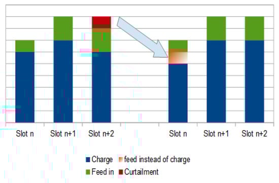
Figure 6.
A graphical illustration of one iteration of Algorithm 2 for lines between 23 and 35.
5.2. Obtained Results
The two policies mentioned above (see Algorithms 1 and 2) were evaluated by setting up a simulation environment that satisfies all the technical characteristics and constraints of the PoC system, where a continuous load of 500 W was considered during all timeslots of the simulation, such that each timeslot was taken to be one hour. This value was calculated by taking the average values of the typical German household H0 load profiles (https://www.bdew.de/energie/standardlastprofile-strom/).
We start by analyzing the charging behavior of ESS, which is illustrated in Figure 7 and Table 6. The minimum value for the “Naive” policy (see Figure 7a) arises from discharging the ESS to satisfy the load of 500 W during hours without forecasts. On the contrary, the “Loss Avoidance” policy (see Figure 7b) selectively discharges the ESS to reserve enough charging capacity for later. The maximum value can be considered as a spike which is confirmed by the plots’ upper whiskers. The amount of energy charged by the “Loss Avoidance” policy during the observation period is 753 kWh higher.
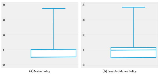
Figure 7.
Obtained results for charging ESS.
Table 6.
Obtained statistical values of Figure 7.
Figure 8 and Table 7 illustrate the analysis results for the energy fed into or drawn from the grid. Those results show identical minimal and maximal values caused by the limitations of the system. Minimal value is caused by satisfying the load of 500 W during hours of no generation as well as empty storage, whereas maximum value indicates that both algorithms exhaust the maximum feed-in at certain timeslots. The box illustrates the middle 50% of the values and shows that the “Loss Avoidance” policy tends to provoke higher values. This is emphasized by the mean and the upper quartile marking the highest single value of 75% of the data.
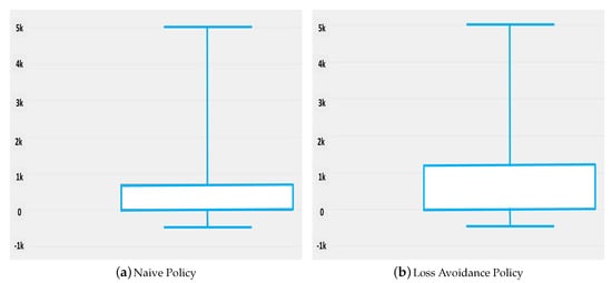
Figure 8.
Obtained results for feed-in to the power grid.
Table 7.
Obtained statistical values of Figure 8.
Charging and feed-in (Figure 7 and Figure 8) provide a good indication of a particular algorithm’s behavior. The comparison of curtailed generation (see Figure 9 and Table 8) adds additional insights regarding whether better irradiance exploitation could be realized. Here, the amount of energy that could have been generated but had to be curtailed due to system restrictions is logged for every timeslot. Note that the number of zero values is slightly higher for the “Loss Avoidance” policy. Furthermore, the maximum theoretical generation during the simulation runtime is calculated to be 1506 kWh.
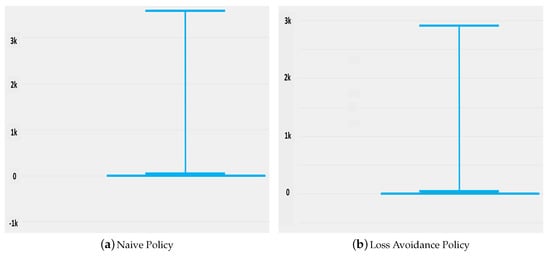
Figure 9.
Obtained results for curtailing excess generation of solar panels.
Table 8.
Obtained statistical values of Figure 9.
The conclusion to draw while analysing Figure 9a,b is the fact that generation needs not be curtailed in 91.6% (i.e., the ratio of 127 kWh to 1506 kWh) of the hours for the “Loss Avoidance” policy, and in 84.4% (i.e., the ratio of 235 kWh to 1506 kWh) of the hours for the “Naive” policy. The identical, seemingly high maximum value is a consequence of peak days during summer, and does not justify changes to the hardware like ESS enlargement. The comparison of the sum values in contrast shows the achieved advantages of our proposed policy. The utilization of additional 1080 kWh was enabled by changing the charge policy from “Naive” to ”Loss Avoidance”. Those improvements are estimated about 8.4% of curtailment for the “Loss Avoidance” policy during the observation period with respect to 15.6% of curtailment for “Naive”.
To study the impact of forecast precision on the quality of the decisions made by proposed Algorithm 2, distortions were added to the data to generate imprecise ’forecasts’. Since predictions can in general tend to underestimate, overestimate, or scatter around real values, these possibilities were taken into account and analyzed. To simulate an underestimating prediction, a normal distributed random factor with a mean of 0.9 and a standard deviation of 10% were considered. The mean for the overestimating scenario was chosen to be 1.1. To generate variation around the real value, 1.0 is taken as the mean for the Deviation scenario. Table 9 illustrates the energy drawn from and fed into the grid, as well as the net value, all expressed in Wh, by taking into account five different scenarios: No predictions, Optimal predictions, Overestimated and Underestimated predictions, and Deviations. Apart from the “No predictions” scenario, the results obtained by the other three scenarios, namely, Overestimated, Underestimated, and Deviation were quite comparable, which, in turn, were close to the results of the Optimal predictions. Even with this discrepancy between predicted and actual generation, Algorithm 2 is capable of outperforming the simple-charge controller (e.g., Algorithm 1) in terms of minimizing the curtailment of generation, which is the reason for the higher net values of the grid meter.
Table 9.
Impact of forecast prediction on generation and feed-in in Wh for the different scenarios.
Figure 10 shows the charging behavior of the different considered scenarios, where the right and left vertical axes denote total charged energy in the ESS (Wh) and charging power (W), respectively. Minimal, maximal, and mean values are related to the left axis, whereas the sum values to the right axis. Usage of the “Loss Avoidance” policy provokes higher net charge, and much higher discharge rates regardless of prediction discrepancies. The higher net value results from better generation utilization on the one hand, but, on the other hand, they are the result of loss of load. The degree of efficiency for charging and discharging is both 93%, so if energy is stored and then fed into the grid, only 86.49% of the generated energy reaches the grid. This adds up and increases the net charge value as the amount of energy is measured before charging and after discharging. The higher discharge rates are clearly a result of strategic planning. For Algorithm 1, the maximum discharge is 500 W to satisfy the equally high load during times of no generation, whereas Algorithm 2 deliberately discharges the ESS to reserve future charging capacity in order to prevent generation curtailment.
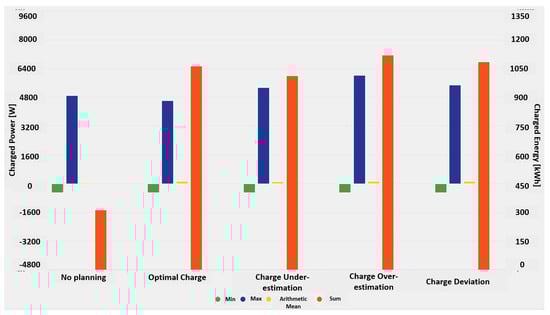
Figure 10.
Differences in charging behavior for the different scenarios.
Consequently, this gives us the conclusion that, despite some discrepancies in forecasting, those have no significant impact on the decisions taken by Algorithm 2, hence demonstrating its robustness.
6. Conclusions
In this paper, we first presented a methodology to forecast the power generation of photovoltaic systems. To this end, we carried out a Pearson’s correlation evaluation and analyzed the different parameters in order to identify the most relevant ones influencing power generation. We then used those parameters and trained neural networks using three types, FFNN, RBFN, and NEAT. Furthermore, we carried out analysis to measure the forecasts’ inaccuracies and showed that NEAT provides the best forecasts.
The corresponding trained network is then used as a forecasting module for a novel energy-management policy that takes optimized decisions on when to charge/discharge the energy storage system and feed into and draw electricity from the power grid. Those decisions were devised in order to reduce power-generation curtailment as much as possible. As a proof of concept, we considered a Fenecon production system and carried out simulations in order to compare both simple and heuristics-based policies proposed in this paper. Simulation results show that the heuristics-based policy outperformedthe naive one by 8% thanks to the incorporated forecasts of PV power generation.
Author Contributions
Conceptualization, R.B. and H.d.M.; methodology, R.B.; software, R.B.; validation, R.B., and H.d.M.; formal analysis, R.B.; investigation, R.B and H.d.M.; resources, H.d.M.; writing—original draft preparation, R.B.; writing—review and editing, R.B. and H.d.M.; supervision, R.B. and H.d.M.
Funding
This research received no external funding.
Acknowledgments
The authors of this paper would like to show their gratitude to Lukas Mueller for his contributions to this paper.
Conflicts of Interest
The authors declare no conflict of interest.
Abbreviations
The following abbreviations are used in this manuscript:
| GHI | Global Horizontal Irradiation |
| RES | Renewable-Energy Sources |
| DSO | Distribution-System Operator |
| EMS | Energy-Management System |
| ANN | Artificial Neural Network |
| RBFN | Radial Basis Function Neural Network |
| FFNN | Feed Forward Neural Network |
| NEAT | NeuroEvolution of Augmenting Topologies |
References
- Adnan, A. Renewable Energy in Cities; Technical Report; International Renewable Energy Agency: Abu Dhabi, UAE, 2016. [Google Scholar]
- Fares, R. Renewable Energy Intermittency Explained: Challenges, Solutions, and Opportunities; Technical Report; Scientific American: New York, NY, USA, 2015. [Google Scholar]
- Zhang, C.; Wei, Y.L.; Cao, P.F.; Lin, M.C. Energy storage system: Current studies on batteries and power condition system. Renew. Sustain. Energy Rev. 2018, 82, 3091–3106. [Google Scholar] [CrossRef]
- Oualmakran, Y.; Espeche, J.M.; Sisinni, M.; Messervey, T.; Lennard, Z. Residential Electricity Tariffs in Europe: Current Situation, Evolution and Impact on Residential Flexibility Markets. In Proceedings of the Sustainable Places 2017 (SP2017) Conference, Middlesbrough, UK, 28–30 June 2017. [Google Scholar]
- Campoccia, A.; Dusonchet, L.; Telaretti, E.; Zizzo, G. An analysis of feed-in tariffs for solar PV in six representative countries of the European Union. Sol. Energy 2014, 107, 530–542. [Google Scholar] [CrossRef]
- Rumelhart, D.; Hinton, G.; Williams, J. Learning representations by back-propagating errors. Nature 1986, 323, 533. [Google Scholar] [CrossRef]
- Pearson, K. Notes on the History of Correlation. Biometrika 1920, 13, 25–45. [Google Scholar] [CrossRef]
- Ramakrishna, R.; Scaglione, A.; Vittal, V. A Stochastic Model for Solar Photo-Voltaic Power for Short-Term Probabilistic Forecast; Technical Report; Cornell University Library: New York, NY, USA, 2017. [Google Scholar]
- Ghiassi-Farrokhfal, Y.; Keshav, S.; Rosenberg, C.; Ciucu, F. Solar Power Shaping: An Analytical Approach. IEEE Trans. Sustain. Energy 2015, 6, 162–170. [Google Scholar] [CrossRef]
- Shi, J.; Lee, W.J.; Liu, Y.; Yang, Y.; Wang, P. Forecasting Power Output of Photovoltaic Systems Based on Weather Classification and Support Vector Machines. IEEE Trans. Ind. Appl. 2012, 48, 1064–1069. [Google Scholar] [CrossRef]
- Yona, A.; Saber, A.Y.; Sekine, H.; Kim, C.H. Application of Neural Network to One-Day-Ahead 24 hours Generating Power Forecasting for Photovoltaic System. In Proceedings of the International Conference on Intelligent Systems Applications to Power Systems, Niigata, Japan, 5–8 November 2007. [Google Scholar]
- Aliberti, A.; Bottaccioli, L.; Cirrincione, G.; Macii, E.; Acquaviva, A.; Patti, E. Forecasting short-term solar radiation for Photovoltaic Energy Predictions. In Proceedings of the International Conference on Smart Cities and Green ICT Systems, Funchal, Portugal, 16–18 March 2018. [Google Scholar]
- Adepetu, A.; Keshav, S. Understanding Solar PV and Battery Adoption in Ontario: An Agent-based Approach. In Proceedings of the Seventh International Conference on Future Energy Systems, Waterloo, ON, Canada, 21–24 June 2016; pp. 5:1–5:12. [Google Scholar]
- Adepetu, A.; Alyousef, A.; Keshav, S.; Meer, H.D. Comparing solar photovoltaic and battery adoption in Ontario and Germany: an agent-based approach. Energy Inform. 2018, 1, 6. [Google Scholar] [CrossRef]
- Kazhamiaka, F.; Ghiassi-Farrokhfal, Y.; Keshav, S.; Rosenberg, C. Robust and Practical Approaches for Solar PV and Storage Sizing. In Proceedings of the Ninth International Conference on Future Energy Systems, Karlsruhe, Germany, 12–15 June 2018; pp. 146–156. [Google Scholar]
- Jin, J.; Xu, Y.; Khalid, Y.I.; Hassan, N.U. Optimal Operation of Energy Storage With Random Renewable Generation and AC/DC Loads. IEEE Trans. Smart Grid 2018, 9, 2314–2326. [Google Scholar]
- Xu, Y.; Tong, L. Optimal Operation and Economic Value of Energy Storage at Consumer Locations. IEEE Trans. Automat. Contr. 2017, 62, 792–807. [Google Scholar] [CrossRef]
- Youn, L.; Cho, S. Optimal Operation of Energy Storage Using Linear Programming Technique. In Proceedings of the World Congress on Engineering and Computer Science, San Francisco, CA, USA, 20–22 October 2009. [Google Scholar]
© 2018 by the authors. Licensee MDPI, Basel, Switzerland. This article is an open access article distributed under the terms and conditions of the Creative Commons Attribution (CC BY) license (http://creativecommons.org/licenses/by/4.0/).