Moving Learning Machine towards Fast Real-Time Applications: A High-Speed FPGA-Based Implementation of the OS-ELM Training Algorithm

Abstract

Currently, there are some emerging online learning applications handling data streams in real-time. The On-line Sequential Extreme Learning Machine (OS-ELM) has been successfully used in real-time condition prediction applications because of its good generalization performance at an extreme learning speed, but the number of trainings by a second (training frequency) achieved in these continuous learning applications has to be further reduced. This paper proposes a performance-optimized implementation of the OS-ELM training algorithm when it is applied to real-time applications. In this case, the natural way of feeding the training of the neural network is one-by-one, i.e., training the neural network for each new incoming training input vector. Applying this restriction, the computational needs are drastically reduced. An FPGA-based implementation of the tailored OS-ELM algorithm is used to analyze, in a parameterized way, the level of optimization achieved. We observed that the tailored algorithm drastically reduces the number of clock cycles consumed for the training execution up to approximately the 1%. This performance enables high-speed sequential training ratios, such as 14 KHz of sequential training frequency for a 40 hidden neurons SLFN, or 180 Hz of sequential training frequency for a 500 hidden neurons SLFN. In practice, the proposed implementation computes the training almost 100 times faster, or more, than other applications in the bibliography. Besides, clock cycles follows a quadratic complexity $O({\tilde{N}}^2)$, with $\tilde{N}$ the number of hidden neurons, and are poorly influenced by the number of input neurons. However, it shows a pronounced sensitivity to data type precision even facing small-size problems, which force to use double floating-point precision data types to avoid finite precision arithmetic effects. In addition, it has been found that distributed memory is the limiting resource and, thus, it can be stated that current FPGA devices can support OS-ELM-based on-chip learning of up to 500 hidden neurons. Concluding, the proposed hardware implementation of the OS-ELM offers great possibilities for on-chip learning in portable systems and real-time applications where frequent and fast training is required.

1. Introduction

There is a current trend to implement hardware on-chip learning for applications such as facial recognition, pattern recognition and complex learning behaviors. As an example, ref. [1] used real-time sequential learning in mobile devices for face recognition applications; ref. [2] proposed a real-time learning of neural networks for the prediction of future opponent robot coordinates; ref. [3] designed an ASIC on-chip learning to learn and extract features existing in input datasets, intended to embedded vision applications; or [4], that implemented a real-time classifier for neurological signals.

The Extreme Learning Machine (ELM) algorithm possesses many aspects that makes it suitable for any real-time or custom hardware implementation. It has a reduced and fixed training time along with an extremely fast learning speed that allows determinism in the computation time and, thus, a great advantage compared to previous well-known training methods as gradient descent [5]. The ELM algorithm is based on Single Layer Feedforward Neural Network (SLFN), using random hidden layer weights and a linear adjustment for the output layer [6,7,8]. The result is a simple training procedure that has been applied to a wide range of applications as electricity price prediction [9], prediction of energy consumption [10], power disaggregation [11], soldering inspection [12], computation of friction [13], non-linear control [14], fiber optic communications [15], or epileptic EEG detection [16]. However, the ELM algorithm is essentially a batch learning method usually running under PC, and only some approaches use it on real-time hardware to compute the on-line working flow, as in [17] where an embedded FPGA estimated the speed for a drive system.

Liang et al. [18] proposed a modified version of the ELM, namely On-line Sequential ELM (OS-ELM), best suited to handle incremental datasets, which is the most natural way of learning in real-time contexts. This learning algorithm keeps the reduced and training time of the original ELM, allowing determinist computation time along other prominent features as: very fast adaptation and convergence speed, acceptance of input chunks of different sizes, high generalization capability, good accuracy, high structural flexibility and only one operating parameter, the number of hidden nodes.

Diverse OS-ELM sequential learning applications have been proposed to date. As an example, ref. [19] adapted an automatic gesture recognition model to new users, getting high recognition accuracy. In a Wi-Fi based indoor positioning application, ref. [20] addressed the problem of obtaining an adaption, in a timely manner, to environmental dynamics; ref. [21] addressed the problem of overcoming the fluctuation problem, and [22] handled the dimension changing problem caused by the increase or decrease of the number of APs (Access Points). In [23], they developed a robust safety-oriented autonomous cruise control based on the Model Predictive Control (MPC) technique; ref. [24] addressed the pedestrian dead-reackoning problem at indoor localization; ref. [25] addressed the problem of detecting attacks in the advanced metering infrastructure of a smart grid; and [26] used OS-ELM to propose an algorithm for facial expression recognition. It can be stated that, nowadays, OS-ELM is used to handle either sequential arrival of data, or large amounts of data.

However, there are currently emerging online learning applications which need real-time handling of data streams. These applications use the OS-ELM in the strict real-time sense. As an example, Chen et al. [27] used an ensemble of OS-ELMs and phase space reconstruction to recognize different types of flow oscillations and accurately forecast the trend of monitored plant variables. It was intended as a support for the operation of nuclear plants, and provided that the prediction time may not be long for operators to take action, they used a sample interval of 0.1 s, time in which the prediction model can be adjusted according to last newly acquired data. Besides, Li et al. [28] built an EOS-ELM-based model to predict the post-fault transient stability status of power systems in real time. Transient stability is a very fast phenomenon that requires a corrective control action within short period of time (<1 s), making it essential a real time fast and accurate detection of unstability. Note that these applications are potentially implementable in hardware using reconfigurable devices as FPGAs, and, in turn, many other real-time applications are suitable to be adapted to the sequential learning [29,30,31,32]. Futhermore, even online learning applications with non-stationary and/or imbalanced streaming data can be managed by OS-ELM-based algorithms [33,34,35]. Although, obviously, there are applications that cannot be implemented on FPGA since their limiting resources, as the implementation of attention mechanisms in remote sensing image pixel-wise classification [36], acoustic adaptation models addressing the presence of microphone mismatch in Automatic Speech Recognition (ASR) systems [37], or the prediction of infectious diseases [38].

As seen above, the use of on-chip learning systems is an emerging trend. These real-time applications will require the implementation of neural networks incorporating an online real-time training, especially on portable hardware systems. In this context, in which the sequential arrival of new training data can be handled as an incremental training dataset, the on-line sequential learning is the most adequate way of learning. Thus, the on-line sequential OS-ELM algorithm appears as a good candidate for these real-time hardware implementations, provided that it keeps a reduced and fixed training time, as ELM, and has a very fast adaptation and convergence speed along with a low number of parameters [18]. However, the OS-ELM algorithm has been usually used in the same manner in real-time scenarios than in the handling of incrementally big datasets, computationally speaking. We wonder if the computation of the OS-ELM could be optimized for the specific case of real-time applications, because achieving shorter training times for this case could open the door of real-time learning to a broad range of new applications.

This paper explores the optimization of the OS-ELM training time when it is used in real-time scenarios. As real-time learning generally requires training the neural network for each new incoming training pattern (instead of chunks), we propose the ’one-by-one training’ of the neural network as the specific condition to be used for the optimization of the OS-ELM computing. This condition enables a simplification in the OS-ELM computing. An analysis of the proposed FPGA-based implementation was conducted in a parameterised way to assess the level of optimization achieved and the weak points of the proposed implementation. The main contributions of this paper are as follows:

• We identify that training the neural network one training pattern at a time is a specific condition of real-time learning applications. We use this condition to simplify the OS-ELM computation for the real-time case, as it enables to follow some mathematical simplifications that avoid using inverse matrices during computation.
• We propose an FPGA-based on-chip learning implementation following one-by-one training of a parameterizable SLFN neural network, which is trained using the proposed tailored implementation of the OS-ELM algorithm.
• We analyze the advantages and disadvantages of this approach. It is shown how the proposed implementation improves dramatically the performance while minimizing its resource usage. In addition, the analysis characterizes the resources usage, the limiting hardware resource and highlights the high sensitivity to the data type precision that affects this approach.

The results are applicable to any real-time classification or regression application based on an SLFN neural network. Results also provide a guideline on required resources and level of performance that an FPGA-based OS-ELM can demand.

The rest of the paper is organized as follows. Section 2 introduces the OS-ELM training algorithm. The details of the architecture and the proposed computational method are described in Section 3. Results of the analysis and discussion are presented in Section 4 and Section 5, respectively. Finally, Section 6 concludes the paper.

2. Online Sequential ELM Algorithm (OS-ELM)

The on-line sequential ELM algorithm (OS-ELM) is built on the basis of batch ELM algorithm.

2.1. ELM Algorithm

The ELM batch learning algorithm is a supervised learning machine based on a Single-hidden Layer Feedforward Neural network (SLFN) architecture [6,7,8]. It establishes that the weights linking to the output layer can be analytically determined through the generalized inverse operation when the weights and bias of the hidden neurons are randomly assigned. It avoids the need to tune these hidden neuron parameters.

Let us assume that $({\mathbf{x}}_i,{\mathbf{t}}_i)$ ∈ ${\mathbb{R}}^n\times {\mathbb{R}}^m$; $i=1,\dots ,N$ is a set of N patterns, where ${\mathbf{x}}_i$ is a $n\times 1$ input vector and ${\mathbf{t}}_i$ a $m\times 1$ output vector. If an SLFN with $\tilde{N}$ hidden neurons and activation function $g(x)$ can approximate these N samples with zero error, there exist ${\mathit{\beta }}_i$, ${\mathbf{a}}_i$, and $b_i$ such that

$$f_{\tilde{N}}({\mathbf{x}}_j)=\sum _{i=1}^{\tilde{N}}{\mathit{\beta }}_{i}G({\mathbf{a}}_i,b_i,{\mathbf{x}}_j)={\mathbf{t}}_j,j=1,\dots ,N$$

(1)

where ${\mathbf{a}}_i$ and $b_i$ are the learning parameters of the hidden nodes (being ${\mathbf{a}}_i$ the weight vector connecting the input node to the hidden node and $b_i$ the bias of the hidden node), both randomly selected according to Huang et al. [6], ${\mathit{\beta }}_i$ is the i-th output weight, and $G({\mathbf{a}}_i,b_i,{\mathbf{x}}_j)$ the output of the i-th hidden node with respect to the input vector ${\mathbf{x}}_j$. If the hidden node is additive, it follows that $G({\mathbf{a}}_i,b_i,{\mathbf{x}}_j)=g({\mathbf{a}}_i·{\mathbf{x}}_j+b_i)$. Then, the Equation (1) can be written as

$$\mathbf{H}\mathit{\beta }=\mathbf{T},$$

(2)

where

$$\mathbf{H}=\left[\begin{array}{ccc}G({\mathbf{a}}_1,b_1,{\mathbf{x}}_1)& \dots & G({\mathbf{a}}_{\tilde{N}},b_{\tilde{N}},{\mathbf{x}}_1)\\ ⋮& \ddots & ⋮\\ G({\mathbf{a}}_1,b_1,{\mathbf{x}}_N)& \dots & G({\mathbf{a}}_{\tilde{N}},b_{\tilde{N}},{\mathbf{x}}_N)\end{array}\right]$$

(3)

is called the hidden layer output matrix (being the i-th row of H the output of the hidden layer with respect to the ${\mathbf{x}}_i$ input vector, and the j-th column the output of the j-th hidden node with respect to ${\mathbf{x}}_1$ to ${\mathbf{x}}_N$ input vectors).

Thus, the matrix of output weights, $\mathit{\beta }$, can be estimated as

$$\tilde{\mathit{\beta }}={\mathbf{H}}^{†}\mathbf{T},$$

(4)

where ${\mathbf{H}}^{†}$ is the Moore-Penrose generalized inverse (pseudo-inverse) [39,40] of the hidden layer output matrix $\mathbf{H}$. Note that the learning parameters ${\mathbf{a}}_i$ and $b_i$ do not need to be tuned during training and can be selected randomly.

2.2. OS-ELM Algorithm

In real applications, training data may arrive one-by-one or chunk-by-chunk. In this case, the ELM algorithm has to be modified to make it suitable for online sequential computation [18,39].

The output weight matrix in Equation (4) is a least-squares solution of Equation (2). Considering that $rank(\mathbf{H})=\tilde{N}$, with $\tilde{N}$ the number of hidden neurons, ${\mathbf{H}}^{†}$ can be expressed as

$${\mathbf{H}}^{†}={\left(\begin{array}{c}{\mathbf{H}}^{\mathbf{T}}\mathbf{H}\end{array}\right)}^{-1}{\mathbf{H}}^{\mathbf{T}}$$

(5)

which is often called the left pseudoinverse of $\mathbf{H}$ because of ${\mathbf{H}}^{†}\mathbf{H}={\mathbf{I}}_{\tilde{N}}$. Substituting Equation (5) into Equation (4), a estimation of $\mathit{\beta }$ is given by

$$\tilde{\mathit{\beta }}={\left(\begin{array}{c}{\mathbf{H}}^{\mathbf{T}}\mathbf{H}\end{array}\right)}^{-1}{\mathbf{H}}^{\mathbf{T}}\mathbf{T}$$

(6)

which is the least-squares solution to $\mathbf{H}\mathit{\beta }=\mathbf{T}$. Thus, the sequential implementation of the least-squares solution of Equation (6) results in the OS-ELM.

Given an initial chunk of training data ${\aleph }_0={({\mathbf{x}}_i,{\mathbf{t}}_i)}_{i=0}^{N_0}$ with $N_0\ge \tilde{N}$, considering the ELM batch learning algorithm one need to consider the problem of minimizing $∥\begin{array}{c}{\mathbf{H}}_0\mathit{\beta }={\mathbf{T}}_0\end{array}∥$, which is given by ${\mathit{\beta }}_0={\mathbf{K}}_0^{-1}{\mathbf{H}}_0^T{\mathbf{T}}_0$ where ${\mathbf{K}}_0={\mathbf{H}}_0^T{\mathbf{H}}_0$.

Suppose that a new chunk of data is presented, ${\aleph }_1={({\mathbf{x}}_i,{\mathbf{t}}_i)}_{i=N_0+1}^{N_0+N_1}$, where $N_1$ is the number of samples in the new chunk. Then, it results in a problem minimizing

$$∥\begin{array}{c}\left[\begin{array}{c}{\mathbf{H}}_0\\ {\mathbf{H}}_1\end{array}\right]\mathit{\beta }-\left[\begin{array}{c}{\mathbf{T}}_0\\ {\mathbf{T}}_1\end{array}\right]\end{array}∥$$

(7)

Thus, considering both ${\aleph }_0$ and ${\aleph }_1$, the output weight matrix $\mathit{\beta }$ becomes

$${\mathit{\beta }}_1={\mathbf{K}}_1^{-1}{\left[\begin{array}{c}{\mathbf{H}}_0\\ {\mathbf{H}}_1\end{array}\right]}^T\left[\begin{array}{c}{\mathbf{T}}_0\\ {\mathbf{T}}_1\end{array}\right]\mathrm{where}{\mathbf{K}}_{\mathbf{1}}={\left[\begin{array}{c}{\mathbf{H}}_0\\ {\mathbf{H}}_1\end{array}\right]}^T\left[\begin{array}{c}{\mathbf{H}}_0\\ {\mathbf{H}}_1\end{array}\right]$$

(8)

For sequential learning, ${\mathit{\beta }}_1$ must be expressed as a function of ${\mathit{\beta }}_0$, ${\mathbf{K}}_1$, ${\mathbf{H}}_1$, and ${\mathbf{T}}_1$, not as a function of the original data set ${\aleph }_0$. Thus, ${\mathbf{K}}_1$ can be written as

$${\mathbf{K}}_1=\left[\begin{array}{cc}{\mathbf{H}}_0^T& {\mathbf{H}}_1^T\end{array}\right]\left[\begin{array}{c}{\mathbf{H}}_0\\ {\mathbf{H}}_1\end{array}\right]={\mathbf{K}}_0+{\mathbf{H}}_1^T{\mathbf{H}}_1$$

(9)

and

$${\left[\begin{array}{c}{\mathbf{H}}_0\\ {\mathbf{H}}_1\end{array}\right]}^T\left[\begin{array}{c}{\mathbf{T}}_0\\ {\mathbf{T}}_1\end{array}\right]={\mathbf{H}}_0^T{\mathbf{T}}_0+{\mathbf{H}}_1^T{\mathbf{H}}_1={\mathbf{K}}_1{\mathit{\beta }}_0-{\mathbf{H}}_1^T{\mathbf{H}}_1{\mathit{\beta }}_0+{\mathbf{H}}_1^T{\mathbf{T}}_1$$

(10)

combining Equations (8) and (10), ${\mathit{\beta }}_1$ can be expressed as

$${\mathit{\beta }}_1={\mathbf{K}}_1^{-1}{\left[\begin{array}{c}{\mathbf{H}}_0\\ {\mathbf{H}}_1\end{array}\right]}^T\left[\begin{array}{c}{\mathbf{T}}_0\\ {\mathbf{T}}_1\end{array}\right]={\mathit{\beta }}_0+{\mathbf{K}}_1^{-1}{\mathbf{H}}_1^T\left({\mathbf{T}}_1-{\mathbf{H}}_1{\mathit{\beta }}_0\right)$$

(11)

Iteratively, when the $(k+1)$th new chunk of data arrives,

$${\chi }_{k+1}={\left\{({\mathbf{x}}_i,{\mathbf{t}}_i)\right\}}_{i=1+{\sum }_{j=0}^k{N}_j}^{{\sum }_{j=0}^{k+1}{N}_j},$$

(12)

recursive methods are implemented to obtain an updated solution. We have

$$\begin{array}{cc}\hfill {\mathbf{K}}_{k+1}& ={\mathbf{K}}_k+{\mathbf{H}}_{k+1}^T{\mathbf{H}}_{k+1}\hfill \\ \hfill {\mathit{\beta }}_{k+1}& ={\mathit{\beta }}_k+{\mathbf{K}}_{k+1}^{-1}{\mathbf{H}}_{k+1}^T\left({\mathbf{T}}_{k+1}-{\mathbf{H}}_{k+1}{\mathit{\beta }}_k\right)\hfill \end{array}$$

(13)

${\mathbf{K}}_{k+1}^{-1}$ rather than ${\mathbf{K}}_{k+1}$ is used to compute ${\mathit{\beta }}_{k+1}$ from ${\mathit{\beta }}_k$ in Equation (13). The update formula for ${\mathbf{K}}_{k+1}^{-1}$ is derived using the Woodbury formula [41]

$$\begin{array}{cc}\hfill {\mathbf{K}}_{k+1}^{-1}& ={\mathbf{K}}_k^{-1}-{\mathbf{K}}_k^{-1}{\mathbf{H}}_{k+1}^T{\left(I+{\mathbf{H}}_{k+1}{\mathbf{K}}_k^{-1}{\mathbf{H}}_{k+1}^T\right)}^{-1}·{\mathbf{H}}_{k+1}{\mathbf{K}}_k^{-1}\hfill \end{array}$$

(14)

Let ${\mathbf{P}}_{k+1}={\mathbf{K}}_{k+1}^{-1}$, then the equation updating ${\mathit{\beta }}_{k+1}$ can be written as in Equation (15), which is the recursive formula for computing ${\mathit{\beta }}_{k+1}$.

$$\begin{array}{cc}\hfill {\mathbf{P}}_{k+1}& ={\mathbf{P}}_k-{\mathbf{P}}_k{\mathbf{H}}_{k+1}^T{\left(I+{\mathbf{H}}_{k+1}{\mathbf{P}}_k{\mathbf{H}}_{k+1}^T\right)}^{-1}{\mathbf{H}}_{k+1}{\mathbf{P}}_k\hfill \\ \hfill {\mathit{\beta }}_{k+1}& ={\mathit{\beta }}_k+{\mathbf{P}}_{k+1}{\mathbf{H}}_{k+1}^T\left({\mathbf{T}}_{k+1}-{\mathbf{H}}_{k+1}{\mathit{\beta }}_k\right)\hfill \end{array}$$

(15)

2.3. OS-ELM for One-by-One Incoming Data

In OS-ELM, incoming chunks do not need to be constant in size, but in the special case where trained data are presented one-by-one (that is, when $N_{k+1}=1$), the recursive equations have the following simple format (Sherman–Morrison formula [42])

$${\mathbf{P}}_{k+1}={\mathbf{P}}_k-\frac{{\mathbf{P}}_k{\mathbf{h}}_{k+1}{\mathbf{h}}_{k+1}^T{\mathbf{P}}_k}{1+{\mathbf{h}}_{k+1}^T{\mathbf{P}}_k{\mathbf{h}}_{k+1}}$$

(16)

$${\mathit{\beta }}_{k+1}={\mathit{\beta }}_k+{\mathbf{P}}_{k+1}{\mathbf{h}}_{k+1}\left({\mathbf{t}}_{k+1}^T-{\mathbf{h}}_{k+1}^T{\mathit{\beta }}_k\right)$$

(17)

with ${\mathbf{h}}_{k+1}=[G({\mathbf{a}}_1,b_1,{\mathbf{x}}_{k+1})\cdots G({\mathbf{a}}_{\tilde{N}},b_{\tilde{N}},{\mathbf{x}}_{k+1})]$ the hidden layer output vector for the incoming sample data ${\mathbf{x}}_{k+1}$ [40].

One-by-one training (the system learns one-by-one the incoming training data) is the feeding strategy proposed in this work because, as it will be discussed in Section 5, the use of the simplified Equations (16) and (17) enables a reduction of computational complexity and, thus, a considerable increase in performance.

2.4. Phases of the OS-ELM Algorithm

Although OS-ELM can learn from chunks of different size, note that one-by-one training strategy followed in this work implies that all input data chunks contain only one data sample.

The OS-ELM learning algorithm is computed in two phases: Boosting phase and Sequential phase [40].

2.4.1. Boosting Phase

In this phase, also called Initialization phase, the SLFN is trained using the batch ELM algorithm with an initial data set of training data. Given an initial training set ${\aleph }_0=\{({\mathbf{x}}_i,{\mathbf{t}}_i)$ ∈ ${\mathbb{R}}^n\times {\mathbb{R}}^m$; $i=1,\dots ,N_0\}$, the following procedure is used to boost the learning algorithm:

• Assign randomly the input weights ${\mathbf{a}}_i$ and biases $b_i$ for $i=1,\dots ,\tilde{N}$.
• Calculate the initial hidden layer output matrix ${{\mathbf{H}}_0=[{\mathbf{h}}_1,\cdots ,{\mathbf{h}}_{\tilde{N}}]}^T$, where ${{\mathbf{h}}_i=[g({\mathbf{a}}_1·{\mathbf{x}}_i+b_1),\cdots ,g({\mathbf{a}}_{\tilde{N}}·{\mathbf{x}}_i+b_{\tilde{N}})]}^T$ for $i=1,\dots ,\tilde{N}$.
• Estimate the initial output weight matrix ${\mathit{\beta }}_0={\mathbf{P}}_{\mathbf{0}}{\mathbf{H}}_0^T{\mathbf{T}}_{\mathbf{0}}$, where ${\mathbf{P}}_0={\left({\mathbf{H}}_{\mathbf{0}}^{\mathbf{T}}{\mathbf{H}}_{\mathbf{0}}\right)}^{-1}$ and ${{\mathbf{T}}_0=[{\mathbf{t}}_1,\cdots ,{\mathbf{t}}_{\tilde{N}}]}^T$.
• Set $k=0$.

The training dataset is discarded when the boosting phase is completed. The only condition to this first phase is to require an initial batch of training data equal or greater in size than $\tilde{N}$, the number of hidden neurons of the SLFN. As an example, if there are 50 hidden neurons, it is needed a minimum of 50 input samples to boost the learning.

2.4.2. Sequential Learning Phase

After the boosting phase, the sequential learning phase will then learn one-by-one incoming data. For each incoming input sample $({\mathbf{x}}_i,{\mathbf{t}}_i)$ ∈ ${\mathbb{R}}^n\times {\mathbb{R}}^m$, which is assumed to be presented one-to-one, the following steps are done:

• Calculate de hidden layer output vector ${{\mathbf{h}}_{k+1}=[g({\mathbf{a}}_1·{\mathbf{x}}_i+b_1),\cdots ,g({\mathbf{a}}_{\tilde{N}}·{\mathbf{x}}_i+b_{\tilde{N}})]}^T$.
• Calculate the $(k+1)$th output weight matrix ${\mathit{\beta }}_{k+1}$ based on Equations (16) and (17).
• Set $k=k+1$.

In a similar way than the boosting phase, the incoming data are discarded once the learning procedure have used these data to obtain the ${\mathbf{P}}_{k+1}$ and ${\mathit{\beta }}_{k+1}$ matrices.

This sequential learning training phase is repeated continuously for each new on-line incoming input pattern.

3. Hardware Architecture

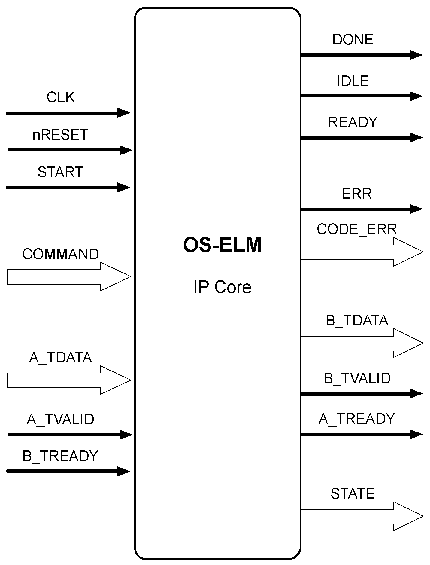
The proposed hardware implementation is conceived as an IP (Intelectual Property) core. Its signal interface definition enables it as a standalone module, or as a peripheral of a more complex System on Chip, embedded microprocessor, etc. This approach, along with its capability of being customised for specific needs, allows its use in many different hardware applications.

3.1. Main Blocks

The IP core is structured in the following four main blocks:

• OSTRAIN_MODULE: Is the SLFN training block. It updates the matrix of output weights according to the last incoming training data sample.
• ANN_MODULE: Implements the on-line working mode for the SLFN. It calculates the output data corresponding to the last incoming input data. This block works only after the module initialization, when valid output weights are available.
• RAM memories: These blocks are shared by different computation units and perform data storage.
• Data flow control state machines and glue logic.

3.2. Working Modes

The most important blocks are OSTRAIN_MODULE and ANN_MODULE, the former performs two different working modes and the latter performs only one working mode. These three working modes are the following:

-

Initialization mode. The module OSTRAIN_MODULE is initialized using the external signal interface. This initialization consists on the load of the initial matrices ${\mathbf{P}}_0$ and ${\mathit{\beta }}_0$, calculated in the boosting phase of the OS-ELM algorithm. Note that the calculation of these matrices reside anywhere out of this IP core, and the results are transfered to the OSTRAIN_MODULE to enable it to perform the sequential learning phase of OS-ELM. In addition, the matrices of hidden weights $\mathbf{W}$ and biases $\mathbf{b}$ of the hidden nodes are also transfered as part of the initialization. Once completed the initialization, the core can enter in another working mode, never before.

-

Training mode. The module OSTRAIN_MODULE performs the learning phase of the OS-ELM training algorithm following the steps in Section 3.4. In this mode, each new incoming input data $({\mathbf{x}}_{k+1},{\mathbf{t}}_{k+1})$ is used to learn and update the internal matrices to ${\mathbf{P}}_{k+1}$ and ${\mathit{\beta }}_{k+1}$. That implements one-by-one training strategy.

-

Run mode or on-line mode. In this mode, the input data ${\mathbf{x}}_i$ are fed into the SLFN neural network system, and the output is computed according to the network topology and the current output weights matrix, ${\mathbf{y}}_i={\mathbf{h}}_{k+1}^T·\mathit{\beta }$. Input data are also fed in a one-by-one approach, that is, when the module ANN_MODULE accepts one input sample, it computes and serves the corresponding output before accepting a new input (unless the admission of the incoming input is externally forced, cancelling the pending computation).

3.3. IP Core Signal Interface

The external core signal interface in Xilinx FPGAs used to follow proprietary protocol specifications as AXI4 [43,44], AXI4-Lite or AXI4-Stream [44,45]. In this work it has be selected an AXI4-Stream protocol to optimize the performance of the initialization mode. However, note that the performance reported in this paper refers to the sequential phase of the OS-ELM training. As the sequential phase of the implementation only needs to load just one input pattern each sequential training iteration, the protocol interface has pretty no influence on performance when the core is running the training mode (as it was checked in an early implementation phase). Therefore, for replication purposes it is important to note that it can be expected to achieve similar results, for the sequential training mode, regardless of the protocol specification selected for the core signal interface (e.g., AXI4 or AXI4-Lite memory-mapped protocols).

The external signal interface used in the IP core is outlined in Figure 1 where thin black arrows are signal lines and white thick arrows represent buses and bunches of signals.

The signal lines START, DONE, READY, and IDLE constitute the block-level interface port signals. These signals control the core independently of any port-level I/O protocol. These signals just indicate when the core block can start processing data (START), when it is ready to accept new inputs (READY), if the core block is idle (IDLE) and if the operation has been completed (DONE).

In turn, input and output data ports follow a handshaked data flow protocol based on an AXI4-Stream [43,44,45], acting as single unidirectional channels, only supporting one data stream, and not implementing side channels. The lines A_TVALID, A_TREADY and the bus A_TDATA constitute the data port for the input stream, while the lines B_TVALID, B_TREADY and the bus B_TDATA constitute the data port for the output stream. TVALID and TREADY lines determine when the information is passed across the interface, and TDATA is the payload, which transports the data from a source to a destination. This two-way flow control mechanism enables both master and slave to control the rate at which the data is transmitted across the interface.

Implementing input and output data ports as streams enables the interface to be more simple while, at the same time, the performance of the initialization mode is better optimized. This kind of interfaces tend to be more specialized around an application, as in this case. Thus, the OS-ELM learning IP core can manage the application data flow without requiring addressing, typical in memory-mapped protocols. This stream port-level interface has certain advantages: it provides an easy and efficient manner to move data between the IP cores, high-speed streaming data, and a more simple external interface.

The rest of the hardware signals are used as application-signaling. The COMMAND bundle of lines enables to request entering on initialization, training or on-line working modes. The STATE bundle of signals allows to monitor application state information, as the current working mode or the initialized state of the core, amongst others.

3.4. Computation of the OS-ELM Algorithm

The proposed IP hardware core implements the sequential learning phase of the OS-ELM algorithm. In other words, it is focused on updating the output weights matrix $\mathit{\beta }$ for each new iteration.

3.4.1. Algorithm Description

During the IP core initialization, the ${\mathbf{P}}_0$ and ${\mathit{\beta }}_0$ matrices are passed as input parameters along with the hidden weights ${\mathbf{a}}_i$ and the biases $b_i$ of the hidden nodes. This initialization is mandatory to the IP core so that it can be fully functional and begin accepting any input data.

Algorithm 1 reflects the steps in which the computation of ${\mathbf{P}}_{k+1}$ and ${\mathit{\beta }}_{k+1}$ was performed. This computational procedure follows the Equations (16) and (17), using a one-by-one feeding of the learning algorithm.

Algorithm 1 Pseudocode of a OS-ELM iteration

Input:    ${\mathbf{x}}_{k+1}$→ Input data training sample   ${\mathbf{P}}_k$→k-th iteration of $\mathbf{P}$ matrix   ${\mathit{\beta }}_k$→k-th output weights matrix    Output:    ${\mathbf{P}}_{k+1}$, ${\mathit{\beta }}_{k+1}$ 1:    ${\mathbf{h}}_{{k+1}_{{}_{(\tilde{N}\times 1)}}}={[g({\mathbf{a}}_1·{\mathbf{x}}_{k+1}+b_1),\cdots ,g({\mathbf{a}}_{\tilde{N}}·{\mathbf{x}}_{k+1}+b_{\tilde{N}})]}^T$ 2:    $tmp{1}_{{}_{{}_{(\tilde{N}\times 1)}}}={\mathbf{P}}_{k_{{}_{(\tilde{N}\times \tilde{N})}}}·{\mathbf{h}}_{{k+1}_{{}_{(\tilde{N}\times 1)}}}$ 3:    $tmp{2}_{{}_{{}_{(1\times \tilde{N})}}}={\mathbf{h}}_{{k+1}_{{}_{(1\times \tilde{N})}}}^T·{\mathbf{P}}_{k_{{}_{(\tilde{N}\times \tilde{N})}}}$ 4:    $tmp{3}_{{}_{{}_{(\tilde{N}\times \tilde{N})}}}=tmp{1}_{{}_{{}_{(\tilde{N}\times 1)}}}·tmp{2}_{{}_{{}_{(1\times \tilde{N})}}}$ 5:    $val{1}_{{}_{{}_{(1\times 1)}}}=1+{\mathbf{h}}_{{k+1}_{{}_{(1\times \tilde{N})}}}^T·tmp{1}_{{}_{{}_{(\tilde{N}\times 1)}}}$ 6:    $tmp{3}_{{}_{{}_{(\tilde{N}\times \tilde{N})}}}=tmp{3}_{{}_{{}_{(\tilde{N}\times \tilde{N})}}}/val{1}_{{}_{{}_{(1\times 1)}}}$ 7:    ${\mathbf{P}}_{{k+1}_{{}_{(\tilde{N}\times \tilde{N})}}}={\mathbf{P}}_{k_{{}_{(\tilde{N}\times \tilde{N})}}}-tmp{3}_{{}_{{}_{(\tilde{N}\times \tilde{N})}}}$ 8:    $tmp{4}_{{}_{{}_{(1\times \mathrm{ON})}}}={\mathbf{h}}_{{k+1}_{{}_{(1\times \tilde{N})}}}^T·{\mathit{\beta }}_{k_{{}_{(\tilde{N}\times \mathrm{ON})}}}$ 9:    $tmp{4}_{{}_{{}_{(1\times \mathrm{ON})}}}={\mathbf{t}}_{{k+1}_{{}_{(1\times \mathrm{ON})}}}^T-tmp{4}_{{}_{{}_{(1\times \mathrm{ON})}}}$ 10:    $tmp{1}_{{}_{{}_{(\tilde{N}\times 1)}}}={\mathbf{P}}_{{k+1}_{{}_{(\tilde{N}\times \tilde{N})}}}·{\mathbf{h}}_{{k+1}_{{}_{(\tilde{N}\times 1)}}}$ 11:    $tmp{5}_{{}_{{}_{(\tilde{N}\times \mathrm{ON})}}}=tmp{1}_{{}_{{}_{(\tilde{N}\times 1)}}}·tmp{4}_{{}_{{}_{(1\times \mathrm{ON})}}}$ 12:    ${\mathit{\beta }}_{{k+1}_{{}_{(\tilde{N}\times \mathrm{ON})}}}={\mathit{\beta }}_{k_{{}_{(\tilde{N}\times \mathrm{ON})}}}-tmp{5}_{{}_{{}_{(\tilde{N}\times \mathrm{ON})}}}$ ($\tilde{N}$: number of hidden neurons, $\mathrm{ON}$: number of output neurons)

The use of one-by-one training is the natural way to feed learning machines in real-time applications. Besides, its use opens the door of a great simplification in the computation. In fact, one-by-one training enables to compute the OS-ELM training algorithm without the use of matrix inverse operations, contrarily to the feeding chunks case of Equation (15). Thus, the training computation is just carried out by matrix addition, subtraction and multiplication (Algorithm 1).

The computational procedure in Algorithm 1 has been designed to minimize the complexity of matrix operations and the memory usage. Note that the matrix by vector and vector by vector multiplications become the most complex matrix computations required. As shown in the following sections, this simplicity impacts in the increase of performance and decrease of resources usage for the hardware implementation.

The pseudocode in Algorithm 1 shows the matrices and vectors involved in each step together with their dimensions and the matrix operation involved. The temporal matrices $tm{p}_n$ (with n ranging 1 to 5) and their reuse along the computation are also shown.

The computational procedure (Algorithm 1) begins calculating ${\mathbf{h}}_{k+1}$ (which is a vector in our one-by-one feeding case). The sigmoid function has been used as activation function (although the OS-ELM algorithm enables the use of a wide range of activation functions, including those piece-wise linear). This vector along with ${\mathbf{P}}_k$ is needed to obtain the computation of ${\mathbf{P}}_{k+1}$ in step 7, and, in turn, this one along with ${\mathit{\beta }}_k$ is needed to compute ${\mathit{\beta }}_{k+1}$ in step 12.

The computational procedure has been implemented using a sequential architecture. Although this computation can be easily parallelized, thus improving the throughput results, the sequential architecture has been proposed to establish a standard machine which can serve as a reference to subsequent works. In addition, this architecture minimizes both the memory usage and the use of arithmetic hardware blocks, as DSP48E1 in Xilinx FPGA.

3.4.2. Design Considerations

The design allows the definition of floating point units of different precision. That is, the core can be generated using half, single or double precision data types (following the IEEE 754 standard for floating-point arithmetic). It allows to test the design behavior in different conditions with minimal code modifications.

However, note that all the results presented in this work (appart from those of the analysis of the sensitivity to the data type precision) have been obtained for double precision floating-point arithmetic. Smaller floating-point formats produce precision issues, as is shown in Section 4.1.

Concerning the activation function, we implemented the sigmoid function using double precision floating-point arithmetic.

On the other hand, note that any step of the pseudocode in Algorithm 1 can be implemented with at most two nested for loops. Also note that the use of floating point operations implies greater latency than the use of fixed-point operations, specially when floating-point multiply-and-accumulate (MAC) operations are carried out, as is the case of the matrix multiplication steps in the pseudocode. This is the reason why a pipelined design of the implemented loops is needed.

When pipelining, the latency of the iteration is not as important as the initiation interval, which is the number of clock cycles that must occur before a new input can be applied. Accordingly, the initiation interval became the optimizing parameter, and the effort was centered in approximating this parameter as close to one as possible. At this respect, we used the optimization pragma directive PIPELINE, with a target of one cycle in each step of the described computational procedure using for loops. This generates a pipelined design keeping an initiation interval as low as possible, drastically reducing the latency.

Finally, we set the clock period target to 4 ns, to force the compiler to look for the fastest hardware implementation.

These design considerations must be followed, along with the computational procedure described in Algorithm 1, to replicate the implementation.

3.5. System Parameterization

A flexible design was obtained through the use of parameters to define the topology of the SLFN neural network. Thus, multiple tests of the design can be performed with minimal code modifications. The main parameters are:

-

IN: Number of neurons in the input layer. It is the size of the data input vector.

-

$\tilde{N}$: Number of neurons in the hidden layer.

-

ON: Number of neurons in the output layer.

-

FT: Type of floating-point arithmetic used. This defines the floating-point arithmetic precision to be used in the design: half, single or double standard (IEEE 754) floating-point arithmetic.

4. Results

Once defined, the architecture was coded using Xilinx Vivado HLS and Xilinx Vivado Design Suite 2016.2 [46], which was also used to carry out simulations, synthesis and co-simulations. The device used for synthesis and implementation was the Xilinx Virtex-7 XC7VX1140T FLG1930-1, the biggest FPGA device of the Xilinx Virtex-7 family. This choice allows to obtain the SLFN order limitations for OS-ELM training in current FPGAs.

As stated before (Section 3), the coded design is parameterisable, uses pipeling, follows a sequential computation (Algorithm 1) to keep updating the output weights matrix of the SLFN neuronal network, and uses the sigmoid function as activation function.

All results in this section are generated using a one-by-one training strategy, meaning that the system is retrained where a new incoming input pattern arrives.

4.1. Sensitivity to Data Type Precision

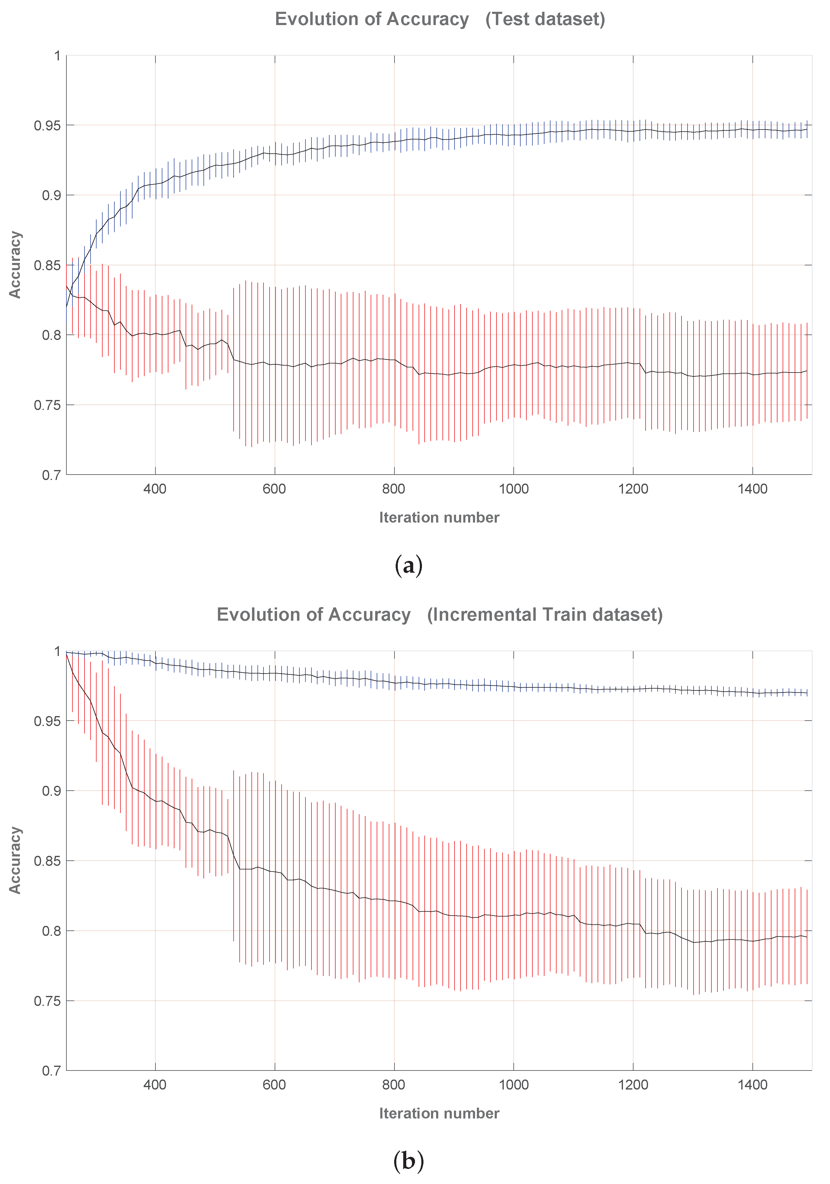
This subsection is focused on showing the great sensitivity to the data type precision of this implementation. To conduct this demonstration, we propose the accuracy evolution analysis of the OS-ELM real-time computation for the image segment classification problem [47]. Note that this accuracy analysis is intended to show how even small-size classification problems can be hardly affected by rounding errors when they are fed back over training iterations.

This analysis was conducted using two designs of different arithmetic precisions. The ’single’ design is based on a 32-bits floating-point arithmetic, and the ’double’ design is based on a 64-bits floating-point arithmetic. Both implementation designs follow the IEEE 754 standard.

The image segment classification problem consists of a database of images randomly drawn from seven outdoor images and consisting of 2310 regions of 3 × 3 pixels. The goal is to recognize each region into one of the seven categories, namely: brick facing, sky, foliage, cement, window, path, and grass, using 19 attributes extracted from each square region.

To manage with this classification problem, we defined an FPGA core implementing a SLFN neural network with 19 neurons in the input layer (IN = 19), seven neurons in the output layer (ON = 7) and 180 neurons in the hidden layer ($\tilde{N}$ = 180).

Following a one-by-one training strategy, each incoming training pattern triggers a sequential training that incorporates knowledge to the system, and thus, the classification accuracy changes as the iterations take place. To clearly illustrate the data type sensitivity, it is interesting to analyze the classification accuracy after each training iteration, namely, evolution of the accuracy. Besides, note that we speak about accuracy in the sense of the proportion of true results, both true positive and true negative, amongst the total number of cases examined.

Testing is done generating 50 random repetitions. In each of these repetitions, the hidden weights and bias matrices are generated randomly. Then, the entire dataset is randomly permuted and, later, partitioned in a test set (810 patterns) and a training set (1500 patterns). In turn, the training set is divided in the boosted training set (250 patterns) and the sequential training set (the rest of the training set, 1250 patterns). The boosted training set is used to compute the initial matrices for the sequential phase. Later, the sequential training set is used to feed (one-by-one) its patterns to the sequential phase of the OS-ELM, calculating the classification accuracy of the learning machine in each iteration, to obtain the evolution of the accuracy. Note that this process is carried out ten times for the same random matrices, that is, ten permutations for each one of the 50 random generations of the hidden weights and biases matrices are performed. In total, each evolution of accuracy is computed from $50\times 10=500$ trials.

Cosimulations were intensively used to collect the results. However, to carry out each cosimulation, it is necessary to transfer some initialization matrices during the initialization step to the FPGA core. These initialization matrices enable the core to perform the sequential training, and proceed from the external execution of the boosting phase of OS-ELM using Matlab R2016a on a PC with a Windows 8.1 operating system. Thus, once the generated matrices are saved from Matlab to a file in a convenient format for the Vivado test bench, they are loaded to properly initialize the FPGA core during cosimulation.

As mentioned before, the evolution of accuracy tracks how the classification accuracy changes over succesive iterations of the sequential OS-ELM learning. Hence, the accuracy for the k-th iteration is the classification accuracy obtained once the sequential training phase of the OS-ELM has trained the ${\aleph }_k=({\mathbf{x}}_k,{\mathbf{t}}_k)$ input. Note that, in this sense, the representations of the evolution of accuracy (Figure 2) starts from iteration 251 because the boosting training phase of the OS-ELM already used $({\mathbf{x}}_i,{\mathbf{t}}_i)$ for $i=1,\dots ,250$.

At each iteration, the classifier performance is measured using both the test set and the training set, resulting in the Test Accuracy and Train Accuracy, respectively. Note that the training set is incremental, growing gradually to $\{({\mathbf{x}}_i,{\mathbf{t}}_i)$$i=1,\dots ,k\}$ for the $k-th$ iteration.

Figure 2a,b show the evolution of accuracy for both the ’single’ and the ’double’ designs, respectively. They have both the same axis limits for comparison purposes. In addition, both ’single’ and ’double’ designs represent the mean and the standard deviation using confidence intervals, provided that they represent the statistical behavior of all repetitions.

In the case of Testing Accuracy (Figure 2a), it can be seen that, as expected, the accuracy of the ’double’ precision design increases as the sequential training evolves. It clearly means that the knowledge of the system improves gradually. Otherwise, the ’single’ precision design does not behaves as expected: the accuracy decreases as the sequential training evolves. Moreover, this accuracy decreases below the value obtained in the boosting phase, implying that the sequential learning goes below the initial knowledge of the system. This behavior is due to a finite precision arithmetic effect caused by the rounding-off errors in the ’single’ design. Note the high standard deviation that this effect introduces in the ’single’ design.

The evolution of the training accuracy relative to the ’double’ design (Figure 2b) shows a slowly decreasing behavior. Also note the small standard deviation for this design when the number of iterations is high. This is a normal behavior considering that the training set grows gradually while the number of hidden neurons, $\tilde{N}$, remains constant. Contrarily, the ’single’ design shows an unexpected behavior, which is that the training accuracy decreases quickly converging to accuracy values below 0.8 and being affected by a great standard deviation. We would be expect the same behavior as in the ’double’ design, but again, it is affected by the feedback of finite precision arithmetic effects.

In the ’double’ case, the Training Accuracy tends to converge to $0.970\pm 0.003$ and the Test Accuracy to $0.946\pm 0.006$. However, the ’single’ case does not interest us because the computation is hardly affected by rounding errors.

It can be concluded from this analysis that the proposed one-by-one OS-ELM training implementation is very sensitive to data type precision and must use double floating-point precision even for small-size problems.

4.2. Hardware Performance Analysis

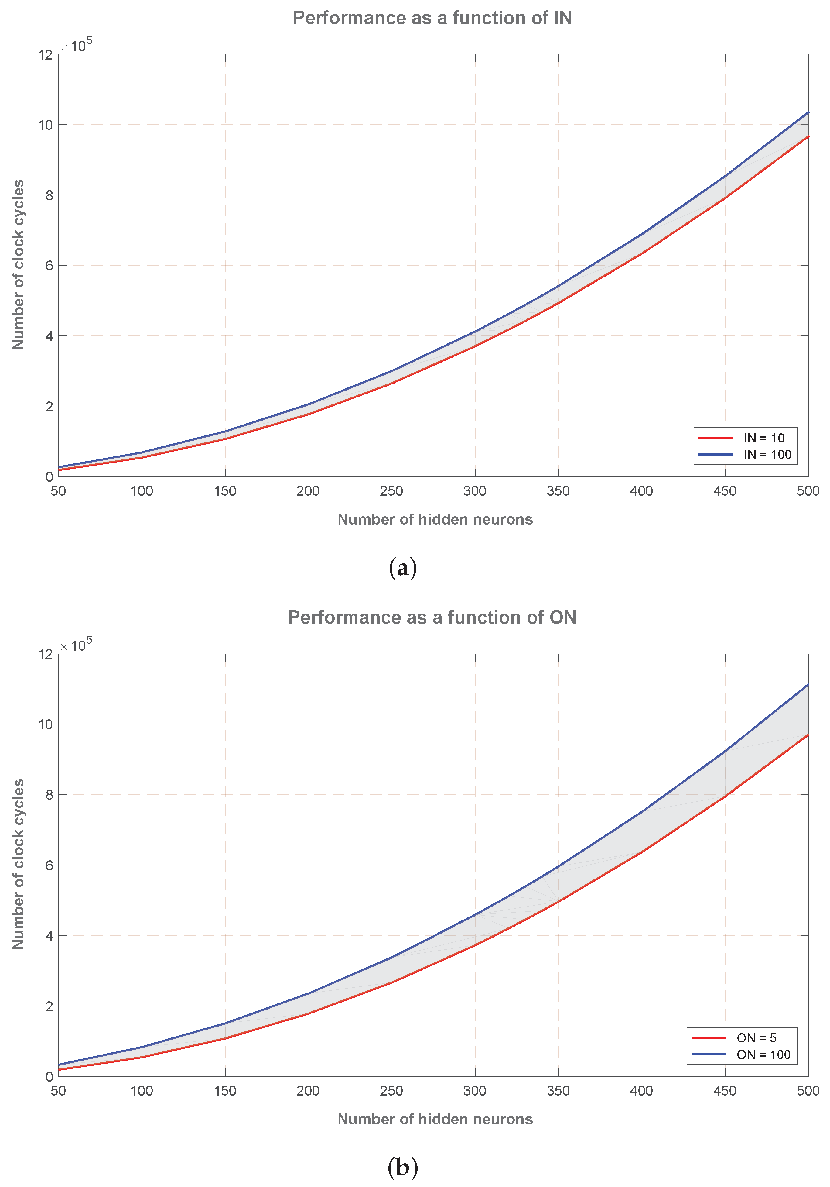
The performance is given by the maximum clock frequency and the required number of clock cycles for computation.

The number of clock cycles follows a quadratic complexity, $O({\tilde{N}}^2)$, as a function of the number of hidden neurons ($\tilde{N}$). Figure 3 illustrates this behavior, and also shows how performance varies when input neurons (IN) ranges from ten to 100 (Figure 3a, using ON = 7), and the corresponding variation when output neurons (ON) range from five to 100 (Figure 3b, using IN = 19).

As can be appreciated in Figure 3, the most significant parameter affecting the required number of clock cycles is the number of hidden nodes ($\tilde{N}$). Besides, Figure 3a shows that an increase in the number of input neurons impacts poorly on performance, and this increment only grows linearly with the number of hidden neurons. Regarding the number of output neurons, Figure 3b, an increase in this parameter double the impact on performance that the same increase in input neurons, and, in the same manner, this impact only grows linearly with the number of hidden neurons.

The minimum allowable clock period is reported in

Table 1. Resource usage and clock period as a function of the number of hidden neurons. Resource usage is indicated both as the number of slices and as the percentage of occupation on a Xilinx Virtex-7 XC7VX1140T FPGA device (IN = 19, ON = 7).

	Hidden Neurons ($\tilde{\mathit{N}}$)
Resources	50	100	150	200	250	300	350	400	450	500
DSP48E	41	41	41	41	41	41	41	41	41	41
BRAM	60	162	306	562	578	1106	1106	2130	2162	2162
FF	32,682	41,196	54,384	63,112	76,273	86,142	99,221	108,291	118,870	130,457
LUT	29,287	43,356	61,964	74,825	111,614	131,160	154,056	170,024	193,454	216,395
DSP48E	1%	1%	1%	1%	1%	1%	1%	1%	1%	1%
BRAM	1%	4%	8%	14%	15%	29%	29%	56%	57%	57%
FF	2%	2%	3%	4%	5%	6%	6%	7%	8%	9%
LUT	4%	6%	8%	10%	15%	18%	21%	23%	27%	30%
Clock Period (ns)	5.05	5.2	5.33	5.33	5.33	5.46	5.33	4.68	5.37	5.46

. It can be observed that the minimum clock period keeps nearly constant, with a value of $5.28\pm 0.16$ ns. This behavior not only applies to the number of hidden neurons ($\tilde{N}$), it produces the same varying the number of input (IN) and output neurons (ON). Thus, we can use 5.3 ns as a constant value for the minimum allowable period on this architecture.

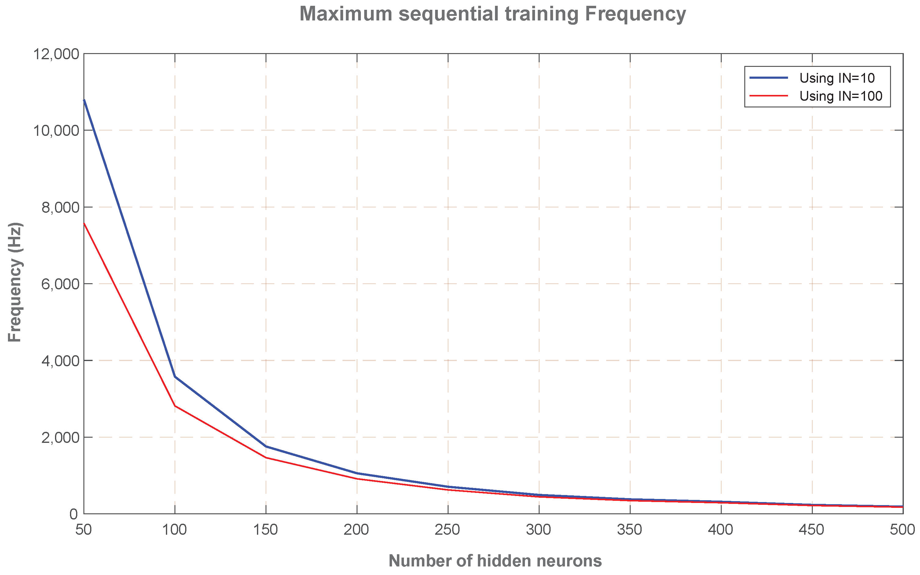
Using the required number of clock cycles and the minimum clock period, the maximum frequency of operation for the sequential training of the OS-ELM learning algorithm can be obtained. Figure 4 represents this maximum frequency of operation, as a function of the number of hidden neurons ($\tilde{N}$), for the cases of ten and 100 input neurons (IN). This frequency must be interpreted as the number of sequential trainings per second that the FPGA core can carry out, as a peak performance. As an example, we can see that for a SLFN network of 50 hidden neurons ($\tilde{N}$ = 50) and 100 input neurons (IN = 100), it is possible to train the incoming data at the rate of 7.58 kHz (7580 input patterns per second).

4.3. Hardware Resources Analysis

The analysis of resources is based on the internal FPGA device blocks: DSP48E blocks, slices containing LUT blocks for general logic, Flip-Flops, and RAM blocks for memory storage. The resource usage was measured as a function of the number of neurons in the hidden layer ($\tilde{N}$). Table 1 gathers all these results. To better understand the reported magnitudes, Table 1 shows resources also as a percentage of occupation in the biggest Xilinx Virtex-7 XC7VX1140T FPGA device.

As it can be seen, the design demands 41 DSP48E slices independently of the number of hidden neurons, $\tilde{N}$. Furthermore, the number of DSP slices is independent of the number of input neurons, IN, or output neurons, ON. Note the reduced amount of DSP48E slices needed. Obviously, it has been achieved thanks to the pipelined design of the proposed hardware architecture.

Both the required number of Flip-Flops (FF) and required number of Look Up Tables (LUT) increase linearly with the number of hidden neurons ($\tilde{N}$). The design does not report a considerable amount of FF usage (9% of FF utilization for $\tilde{N}$ = 500). The LUT usage, in turn, approximately triples that of the FF usage (30.4% of LUT occupation for $\tilde{N}$ = 500). The dependency with the input, IN, and output neurons, ON, is very slight compared with that of the number of hidden neurons, $\tilde{N}$ (as a rule of thumb, FF increases 1% when IN increases by ten, while LUTs present a smaller variation).

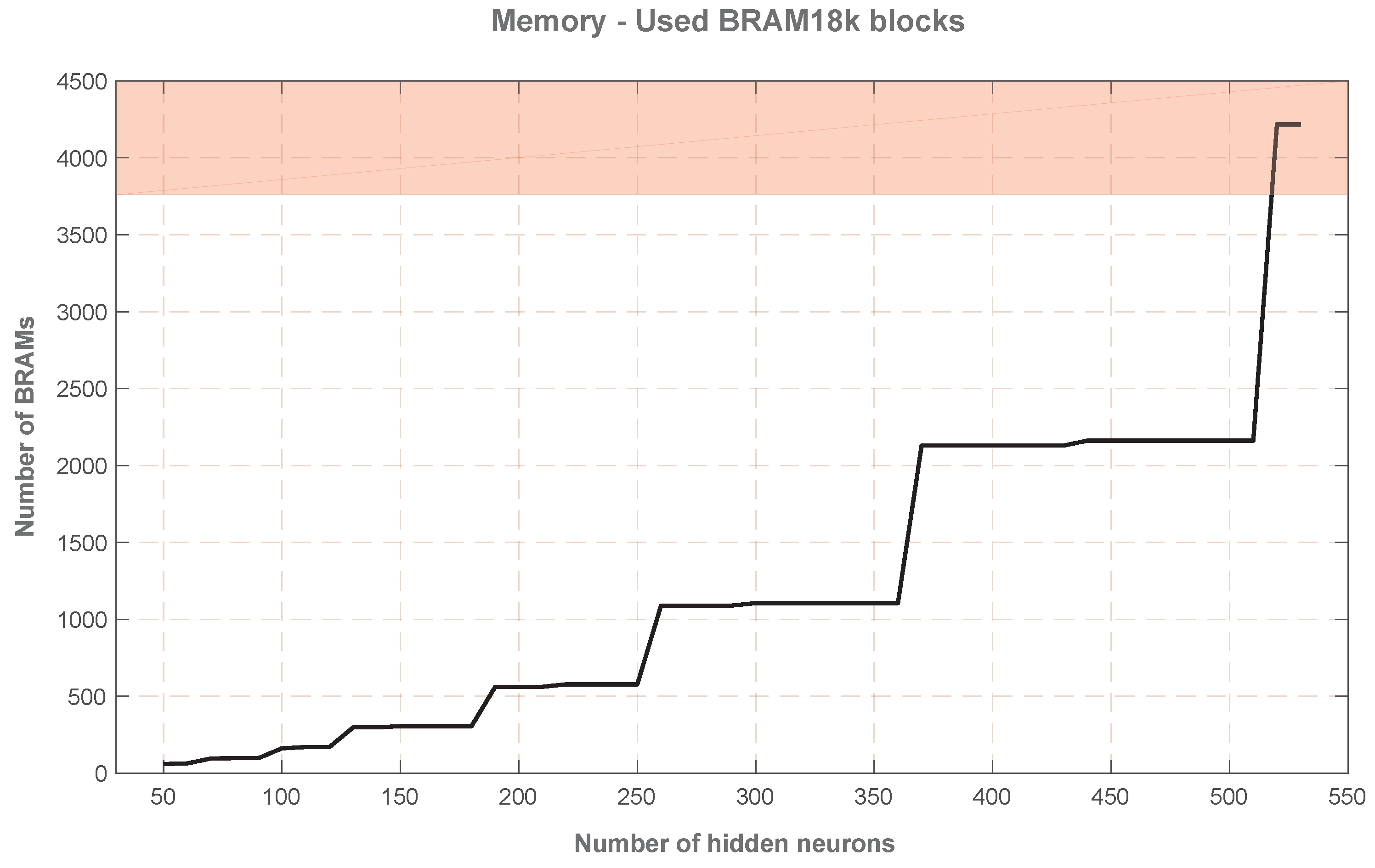
The number of used Block RAMs appears as the limiting factor of this implementation. This is due to the need for internal storage of matrices and vectors, which grow exponentially with the number of hidden neurons, $\tilde{N}$. From 50 to 500 hidden neurons, its BRAM usage varies from 60 to 2162 (1.59% to 57.5% of the available Block RAMs in the biggest device of the advanced Virtex-7 family). This memory usage shows a characteristic ladder shape in Figure 5 since no new memory blocks are reserved until the existing ones are full, and then, the block usage doubles (what is seen in the memory usage as a ladder step). Thus, the maximum amount of distributed memory in current FPGAs (the red zone in Figure 5) determines the maximum implementable SLFN in this architecture, which is just above $\tilde{N}=500$.

5. Discussion

As an on-line sequential learning method, the OS-ELM can face applications with incremental training datasets, permitting to improve the knowledge of the system on-the-fly. This study is centered on the use of this training algorithm in real-time learning applications, where the system has to be trained for each new incoming data pattern.

This real-time on-line sequential training was implemented on a compact and fast circuitry supporting an SLFN neural network. Programmable logic is the more efficient and effective device to carry out this implementation since FPGA devices are cost-effective, have a much shorter design flow and privileges computational optimization.

This work proposes a pipelined sequential hardware implementation on a reconfigurable FPGA device of the Xilinx Virtex-7 Family. This is the biggest FPGA device from the Virtex 7 advanced family, and was selected to be able of evaluating the maximum possible dimension implementable for the OS-ELM training in current FPGAs. Besides, the hardware implementation uses pipelining. The pipelining is mandatory to considerably reduce the total latency of the sequential training (the design uses floating-point arithmetic, following the IEEE 754 standard, having each individual floating-point operation a considerable latency).

Note that this design assumes a one-by-one training strategy (In one-by-one training strategy the system is re-trained each time a new incoming training data input arrives. That is, chunks are of size one) not only because one-by-one is considered a natural way of feeding for real-time applications, but also to achieve a considerably impact on the performance of the hardware implementation. This impact is achieved from the simplification of the update computation of ${\mathbf{P}}_{k+1}$ and $\mathit{\beta }$ matrices, Equations (16) and (17), which enables to use only matrix by vector or vector by vector multiplications for the update computation. Otherwise, when chunks of size larger than one are used, the update computation needs a $\tilde{N}\times \tilde{N}$ matrix inversion, Equation (15), which implies computing a QR decomposition followed by a Triangular Matrix Inversion, which is computationally tough [48]. Thus, the proposed one-by-one training greatly simplifies computation.

To quantify the improvement achieved using one-by-one training simplification, its computational effort must be compared with the computational effort of computing the general chunk feeding expression in Equation (15). The latter case requires other matrix operations, but the most consuming matrix operation is the $\tilde{N}\times \tilde{N}$ matrix inversion, and hence, the number of execution cycles for the matrix inversion may constitute a rough estimation (downward estimation) for this case. With comparison purposes, this value can be obtained from [48], where an optimal FPGA-based implementation of the ELM training was implemented, the number of training clock cycles was expressed analytically, and almost all the computational effort involved the inversion computation. Table 2 compares the number of clock cycles needed for the OS-ELM training using the proposed one-by-one training strategy and chunk feeding (downward estimation obtained from [48]). The comparison is achieved for different number of neurons in the hidden layer. The last row indicates the performance ratio of computing one-by-one strategy respect to the chunk strategy.

Thus, whatever real-time learning application feeding the input training patterns one-by-one, through the proposed architecture, we can get a big difference in performance at the expense of losing the ability of feeding chunks. Table 2 shows that a one-by-one strategy reduces the number of clock cycles consumed for training execution as low as around the 1% (below 1% for $\tilde{N}\ge 200$), which means around 100 times faster, and note that this value constitutes a conservative estimation. Hence, even for feeding small-size chunks it would be more efficient to use the proposed architecture and train one-by-one each input pattern of the chunk. Note the great advantage obtained using the proposed architecture.

On the other hand, it must be highlighted that, despite the simplification in the computation, the proposed architecture keeps the great sensitivity to the data type precision typical of the chunk OS-ELM sequential phase training. It has been illustrated, in Section 4.2, that even facing a small-size problem the proposed architecture needs to use the double (Double format follows double precision IEEE 754 floating-point standard) floating-point precision data type to avoid finite precision arithmetic effects. Section 4.2 details how using the double floating-point format the system learns on-the-fly normally (classification accuracy converges to $97.0\%\pm 0.3\%$ for training, and to $94.6\%\pm 0.6\%$ for testing). However, when using a single floating-point format (Single format follows single precision IEEE 754 floating-point standard.) the obtained results become very different while they were expected to be the same (in fact, in the single case the classification accuracy evolved to worse values than those obtained at the boosting phase). This is because the computation is affected of finite precision arithmetic effects (even using a 32-bits floating-point format) fed back between iterations. As it can be seen, the single floating-point format is not providing enough precision to compute OS-ELM sequential phase training, only the double floating-point format does. It is a limitation to take into account.

Concerning hardware resources, it should be noted that the number of DSP48E1 slices used in the proposed architecture is very low: 41 DSPs. It means a 1.22% of the available DSPs in the biggest device of the advanced Virtex-7 family. Moreover, this usage is independent of all the SLFN parameters (number of hidden neurons, $\tilde{N}$, number of inputs, IN, and number of outputs, ON). This is achieved thanks to the pipelined design of the proposed hardware architecture (Section 3.4). In the same line, the use of FFs grows linearly with the number of hidden nodes; however, it does not report a considerable amount of usage (9% of FFs utilization for $\tilde{N}=500$). In turn, the LUT usage also grows linearly with the number of hidden neurons (Section 4.3), up to a 30.4% of LUT occupation for $\tilde{N}=500$. As a rule of thumb, the proposed architecture uses three times more LUTs than FFs.

However, the resource that really limits the size of the implementation is the Block RAM memory. Its occupation varies exponentially with the number of hidden neurons: from 50 to 500 hidden neurons its BRAM usage varies from 60 to 2162 (1.59% to 57.5% of the available Block RAMs in the biggest device of the advanced Virtex-7 family). Most of the memory is used to store internal matrices, such as ${\mathbf{P}}_{k+1}$ or ${\mathit{\beta }}_{k+1}$ and other temporary matrices used during computation. As some of these are square matrices, the increase in the number of hidden neurons, $\tilde{N}$, impacts quadratically in the stored values, and thus in the required memory. Given that the memory is the only resource growing exponentially with $\tilde{N}$, it becomes the limiting resource of this hardware implementation, becoming $\tilde{N}=500$ the limit for the biggest SLFN implementable on current FPGAs.

Concerning hardware performance, it can be observed, Section 4.2, that the proposed architecture keeps a minimum clock period nearly constant around 5.3 ns, and that the number of required clock cycles for execution follows a quadratic complexity, $O({\tilde{N}}^2)$. Besides, an increase in the number of input neurons impacts poorly on performance (with an increment growing linearly with $\tilde{N}$).

However, the peak performance of the proposed OS-ELM implementation is better visualized by the maximum frequency of operation (Figure 4) that can sequentially train. As an example, it can sequentially train: a SLFN of 50 hidden neurons and 100 input neurons at 7.5 kHz (i.e., it can train one-by-one 7500 input patterns per second), or 914 input patterns per second in a 200 hidden neurons SLFN (914 Hz), or 177 input patterns per second with a 500 hidden neurons SLFN (177 Hz). These are really high speed training values that can take place thanks to computational simplification that one-by-one training strategy permit.

As it can be seen, the proposed OS-ELM architecture enables the use of real-time on-chip learning with high sequential re-training frequencies. It would be interesting to estimate how this architecture would impact on the improvement of performance of some works in the bibliography. As an example, Chen et al. [27] used OS-ELM to recognize different types of flow oscillations, and forecast them accurately, as a support for the operation of nuclear plants. They used an ensemble of 15 SLFNs with 40 hidden neurons, 15 input neurons (rolling motion condition), and a re-training frequency of 10 Hz. Using the architecture proposed in this work they could have achieved an OS-ELM sequential training at a rate of above 14 kHz, and for the whole ensemble it could have achieved a sequential training rate of 940 Hz, which is almost 100 times faster than the used by Chen. On the other hand, Li et al. [28] built a real time EOS-ELM (ensemble of OS-ELMs) model to predict the post-fault transient stability status of power systems. They proposed an ensemble consisting of 10 SLFN neural networks with 65 hidden nodes and an optimal feature subset of 7 input neurons. This application requires a very fast corrective control action within a short period of time, ever below 1 s. In this case, our architecture proposal could have achieved a retraining frequency at a rate above 7.23 kHz and then the complete ensemble could have been retrained at 723 Hz frequency, a much higher rate than the 1 Hz used by Li et al. Anyway, note that real-time training applications usually use moderate number of hidden neurons, taking sometimes the advantage of using ensembles to improve accuracy.

Obtained results show remarkable benefits of using the proposed architecture to sequentially train a SLFN with a dedicated circuit approach. This approach provides a high-end computing platform with superior speed performance, being able to compute the on-line sequential training almost 100 times, or more, faster than other applications in the bibliography. That opens the door to a world of possibilities for the real-time on-chip learning.

6. Conclusions

The proposed FPGA-based implementation of the sequential phase of the OS-ELM training would permit to run almost 100 times faster some real-time online learning applications in the bibliography. This high performance are possible thanks to the simplifications in computing that the adoption of one-by-one training strategy entails.

The OS-ELM algorithm has revealed as a good candidate for the hardware implementation of real-time online learning applications, due to its combination of high training speeds and a tight use of resources. However, although this on-chip learning achieve high-speed training ratios (such as 14 kHz for a SLFN with 40 hidden neurons, or 180 Hz for 500 hidden neurons), it only permits hardware implementations of SLFNs of up to 500 hidden neurons on current FPGAs (this value is only limited by the internal distributed memory). In addition, it has limitations regarding data type precision: at least double 64-bits floating-point format must be used to avoid the feedback of finite precision arithmetic effects between iterations, completely distorting the training procedure.

Concluding, it has been shown that the proposed hardware implementation of the OS-ELM offers great possibilities for on-chip learning in neural networks with applications in many different fields.