Acoustic-Based Fault Diagnosis of Commutator Motor


Abstract
1. Introduction
2. Acoustic-Based Fault Diagnosis Technique of the Commutator Motor
2.1. Method of Selection of Amplitudes of Frequency Multiexpanded 8 Groups
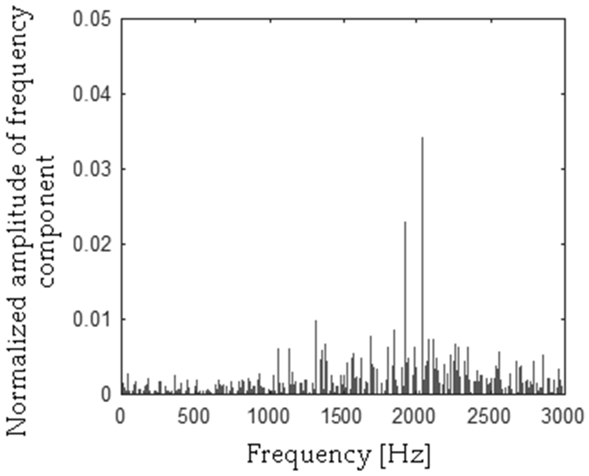
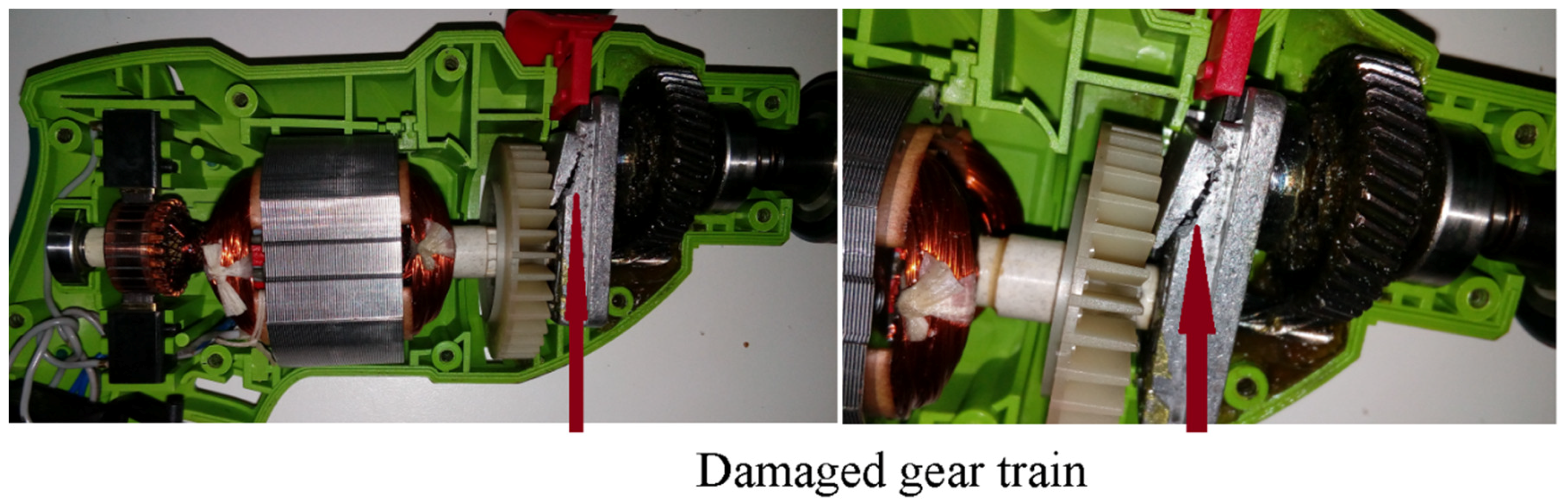
- Compute frequency spectra of acoustic signals of commutator motors (the author used 6 one-second samples for state A, 6 one-second samples for state B, 6 one-second samples for state C, 6 one-second samples for state D). Computed frequency spectrum of state A (healthy CM) was described as vector of 16,384 elements hcm = [hcm1, hcm2, ..., hcm16384]. Computed frequency spectrum of state B (CM with broken rotor coil) was denoted as vector of 16,384 elements cmbrc = [cmbrc1, cmbrc2, ..., cmbrc16384]. Computed frequency spectrum of state C (CM with shorted stator coils) was expressed as vector of 16,384 elements cmssc = [cmssc1, cmssc2, ..., cmssc16384]. Computed frequency spectrum of state D (CM with broken tooth on sprocket) was expressed as vector of 16384 elements cmbts = [cmbts1, cmbts2, ..., cmbts16384]. Computed frequency spectrum of state E (CM with damaged gear train) was expressed as vector of 16,384 elements cmdgt = [cmdgt1, cmdgt2, ..., cmdgt16384].
- Compute differences of computed frequency spectra of states A, B, C, D, E: hcm − cmbrc, hcm − cmssc, cmbrc − cmssc, cmbts − hcm, cmbts − cmbrc, cmbts − cmssc, cmdgt − hcm, cmdgt − cmbrc, cmdgt − cmssc, cmdgt − cmbts.
- Compute absolute values: |hcm − cmbrc|, |hcm − cmssc|, |cmbrc − cmssc|, |cmbts − hcm|, |cmbts − cmbrc|, |cmbts − cmssc|, |cmdgt − hcm|, |cmdgt − cmbrc|, |cmdgt − cmssc|, |cmdgt − cmbts|.
- Select 15 maximum differences of computed frequency spectra of states A, B, C, D, E: max1(|hcm − cmbrc|), max2(|hcm − cmbrc|), …, max15(|hcm − cmbrc|), max1(|hcm − cmssc|), max2(|hcm − cmssc|), …, max15(|hcm − cmssc|), max1(|cmbrc − cmssc|), max2(|cmbrc − cmssc|), …, max15(|cmbrc − cmssc|), max1(|cmbts − hcm|), max2(|cmbts − hcm|), …, max15(|cmbts − hcm|), max1(|cmbts − cmbrc|), max2(|cmbts − cmbrc|), …, max15(|cmbts − cmbrc|), max1(|cmbts − cmssc|), max2(|cmbts − cmssc|), …, max15(|cmbts − cmssc|), max1(|cmdgt − hcm|), max2(|cmdgt − hcm|), …, max15(|cmdgt − hcm|), max1(|cmdgt − cmbrc|), max2(|cmdgt − cmbrc|), …, max15(|cmdgt − cmbrc|), max1(|cmdgt − cmssc|), max2(|cmdgt − cmssc|), …, max15(|cmdgt − cmssc|), max1(|cmdgt − cmbts|), max2(|cmdgt − cmbts|), …, max15(|cmdgt − cmbts|). The result of feature extraction method MSAF-15 is the vector consisted of 1–15 frequency components. Let us see following example using the MSAF-15. There are 5 states of the CM: A, B, C, D, E. Five frequency spectra of acoustic signals of the CM ((FS-A), (FS-B), (FS-C), (FS-D), (FS-E)-frequency spectra of states A, B, C, D, E) were computed. The MSAF-15 computed frequency components 100, 160, 200, 260, 300 Hz for difference |(FS-A) − (FS-B)|. The MSAF-15 computed frequency components 120, 160, 210, 260, 310 Hz for difference |(FS-A) − (FS-C)|. The MSAF-15 computed frequency components 120, 170, 220, 230, 310 Hz for difference |(FS-B) − (FS-C)|. The MSAF-15 computed frequency components 400, 410, 420, 430, 440 Hz for difference |(FS-D) − (FS-A)|. The MSAF-15 computed frequency components 405, 415, 425, 435, 445 Hz for difference |(FS-D) − (FS-B)|. The MSAF-15 computed frequency components 410, 415, 420, 425, 430 Hz for difference |(FS-D) − (FS-C)|. The MSAF-15 computed frequency components 500, 505, 510 Hz for difference |(FS-E) − (FS-A)|. The MSAF-15 computed frequency components 515, 520, 525 Hz for difference |(FS-E) − (FS-B)|. The MSAF-15 computed frequency components 530, 540, 550 Hz for difference |(FS-E) − (FS-C)|. The MSAF-15 computed frequency components 560, 570, 580 Hz for difference |(FS-E) − (FS-D)|. None of common frequency components were selected for the presented example. The MSAF-15-MULTIEXPANDED-GROUPS extends the MSAF-15 method. A parameter called TCoF-TS (Threshold of common frequency components-training sets) was used. This parameter was defined as: TCoF-TS = (number of required common frequency components of analysed training sets)/(number of analysed differences).
- Set the parameter TCoF-TS. This parameter affects the number of common frequency components. Let us consider following example using the MSAF-15-MULTIEXPANDED. Four training sets of acoustic training samples are given: (A1, B1, C1, D1, E1), (A2, B2, C2, D2, E2), (A3, B3, C3, D3, E3), (A4, B4, C4, D4, E4), where A1, A2, A3, A4—denoted 4 acoustic training samples of state A; B1, B2, B3, B4—denoted 4 acoustic training samples of state B; C1, C2, C3, C4—denoted 4 acoustic training samples of state C; D1, D2, D3, D4—denoted 4 acoustic training samples of state D; E1, E2, E3, E4—denoted 4 acoustic training samples of state E. The MSAF-15-MULTIEXPANDED computed frequency components (FS-A1, FS-B1, FS-C1, FS-D1, FS-E1), (FS-A2, FS-B2, FS-C2, FS-D2, FS-E2), (FS-A3, FS-B3, FS-C3, FS-D3, FS-E3), (FS-A4, FS-B4, FS-C4, FS-D4, FS-E4), where FS-A1, FS-A2, FS-A3, FS-A4—denoted 4 frequency spectra of state A, FS-B1, FS-B2, FS-B3, FS-B4—denoted 4 frequency spectra of state B, FS-C1, FS-C2, FS-C3, FS-C4—denoted 4 frequency spectra of state C, FS-D1, FS-D2, FS-D3, FS-D4—denoted 4 frequency spectra of state D, FS-E1, FS-E2, FS-E3, FS-E4—denoted 4 frequency spectra of state E. Next, 40 differences between frequency spectra are computed: |(FS-A1) − (FS-B1)|, |(FS-A1) − (FS-C1)|, |(FS-B1) − (FS-C1)|, |(FS-D1) − (FS-A1)|, |(FS-D1) − (FS-B1)|, |(FS-D1) − (FS-C1)|, |(FS-E1) − (FS-A1)|, |(FS-E1) − (FS-B1)|, |(FS-E1) − (FS-C1)|, |(FS-E1) − (FS-D1)|, ... , |(FS-A4) − (FS-B4)|, |(FS-A4) − (FS-C4)|, |(FS-B4) − (FS-C4)|, |(FS-D4) − (FS-A4)|, |(FS-D4) − (FS-B4)|, |(FS-D4) − (FS-C4)|, |(FS-E4) − (FS-A4)|, |(FS-E4) − (FS-B4)|, |(FS-E4) − (FS-C4)|, |(FS-E4) − (FS-D4)|. Let us consider following example. If we set TCoF-TS = 4/40 = 0.1, then the MSAF-15-MULTIEXPANDED selects frequency components found 4 times for 40 differences. If we set TCoF-TS = 6/40 = 0.15, then the MSAF-15-MULTIEXPANDED selects frequency components found 6 times for 40 differences. The MSAF-15-MULTIEXPANDED found frequency component 160 Hz-6 times, frequency component 210 Hz-4 times. The MSAF-15-MULTIEXPANDED selects 160, 210 Hz (if TCoF-TS = 4/40 = 0.1). The MSAF-15-MULTIEXPANDED selects 160 Hz (if TCoF-TS = 6/40 = 0.15). The MSAF-15-MULTIEXPANDED selects none of frequency components (if TCoF-TS = 8/40 = 0.2). The parameter TCoF-TS depends on analysed signal.
- Select groups of common frequency components. The MSAF-15-MULTIEXPANDED-8-GROUPS used 8 groups. Each group of common frequency components consists of the best frequency components for recognition. Let us analyse following example. There are 4 states of the CM: A, B, C, D (for 5 states it will be similarly). The MSAF-15-MULTIEXPANDED-8-GROUPS found: frequency component 210 Hz (4 times), frequency component 160 Hz (6 times), frequency component 400 Hz (7 times). The frequency component 210 Hz is good for recognition of |(FS-A) − (FS-B)|, |(FS-A) − (FS-C)|, |(FS-B) − (FS-C)|. The frequency component 160 Hz is good for recognition of |(FS-D) − (FS-A)|, |(FS-D) − (FS-B)|, |(FS-D) − (FS-C)|. The frequency component 400 Hz is good for recognition of |(FS-A) − (FS-B)|. Essential frequency components are 210 Hz and 160 Hz. The frequency component 400 Hz is not good for analysis. The essential frequency components 160 Hz and 210 Hz form 1 group of essential frequency components.
- Use 1–8 computed groups.
- Form a feature vector.
2.2. Nearest Neighbour Classifier
2.3. Nearest Mean Classifier
2.4. Self-Organizing Map
2.5. Backpropagation Neural Network
3. Results of Acoustic-Based Fault Diagnosis Technique of the Commutator Motor
4. Conclusions
Funding
Acknowledgments
Conflicts of Interest
References
- Li, Z.X.; Jiang, Y.; Hu, C.; Peng, Z. Recent progress on decoupling diagnosis of hybrid failures in gear transmission systems using vibration sensor signal: A review. Measurement 2016, 90, 4–19. [Google Scholar] [CrossRef]
- Kim, K.C. Analysis on Electromagnetic Vibration for Interior Permanent Magnet Synchronous Motor Due to Temperature and Loads. Adv. Sci. Lett. 2017, 23, 9767–9772. [Google Scholar] [CrossRef]
- Zhao, H.M.; Deng, W.; Yang, X.H.; Li, X.M. Research on a vibration signal analysis method for motor bearing. Optik 2016, 127, 10014–10023. [Google Scholar] [CrossRef]
- Moosavian, A.; Najafi, G.; Ghobadian, B.; Mirsalim, M. The effect of piston scratching fault on the vibration behavior of an IC engine. Appl. Acoust. 2017, 126, 91–100. [Google Scholar] [CrossRef]
- Cruz-Vega, I.; Rangel-Magdaleno, J.; Ramirez-Cortes, J.; Peregrina-Barreto, H. Automatic progressive damage detection of rotor bar in induction motor using vibration analysis and multiple classifiers. J. Mech. Sci. Technol. 2017, 31, 2651–2662. [Google Scholar] [CrossRef]
- Armentani, E.; Sepe, R.; Parente, A.; Pirelli, M. Vibro-Acoustic Numerical Analysis for the Chain Cover of a Car Engine. Appl. Sci. 2017, 7, 610. [Google Scholar] [CrossRef]
- Jafarian, K.; Mobin, M.; Jafari-Marandi, R.; Rabiei, E. Misfire and valve clearance faults detection in the combustion engines based on a multi-sensor vibration signal monitoring. Measurement 2018, 128, 527–536. [Google Scholar] [CrossRef]
- Siljak, H.; Subasi, A. Berthil cepstrum: A novel vibration analysis method based on marginal Hilbert spectrum applied to artificial motor aging. Electr. Eng. 2018, 100, 1039–1046. [Google Scholar] [CrossRef]
- Zurita-Millan, D.; Delgado-Prieto, M.; Saucedo-Dorantes, J.J.; Carino-Corrales, J.A.; Osornio-Rios, R.A.; Ortega-Redondo, J.A.; Romero-Troncoso, R.D. Vibration Signal Forecasting on Rotating Machinery by means of Signal Decomposition and Neurofuzzy Modeling. Shock Vib. 2016, 2016, 1–13. [Google Scholar] [CrossRef]
- Martinez, J.; Belahcen, A.; Muetze, A. Analysis of the Vibration Magnitude of an Induction Motor with Different Numbers of Broken Bars. IEEE Trans. Ind. Appl. 2017, 53, 2711–2720. [Google Scholar] [CrossRef]
- Saucedo-Dorantes, J.J.; Delgado-Prieto, M.; Ortega-Redondo, J.A.; Osornio-Rios, R.A.; Romero-Troncoso, R.D. Multiple-Fault Detection Methodology Based on Vibration and Current Analysis Applied to Bearings in Induction Motors and Gearboxes on the Kinematic Chain. Shock Vib. 2016, 2016, 1–13. [Google Scholar] [CrossRef]
- Li, Y.; Chai, F.; Song, Z.X.; Li, Z.Y. Analysis of Vibrations in Interior Permanent Magnet Synchronous Motors Considering Air-Gap Deformation. Energies 2017, 10, 1259. [Google Scholar] [CrossRef]
- Delgado-Arredondo, P.A.; Morinigo-Sotelo, D.; Osornio-Rios, R.A.; Avina-Cervantes, J.G.; Rostro-Gonzalez, H.; Romero-Troncoso, R.D. Methodology for fault detection in induction motors via sound and vibration signals. Mech. Syst. Signal Process. 2017, 83, 568–589. [Google Scholar] [CrossRef]
- Dong, J.N.; Jiang, J.W.; Howey, B.; Li, H.D.; Bilgin, B.; Callegaro, A.D.; Emadi, A. Hybrid Acoustic Noise Analysis Approach of Conventional and Mutually Coupled Switched Reluctance Motors. IEEE Trans. Energy Convers. 2017, 32, 1042–1051. [Google Scholar] [CrossRef]
- Stief, A.; Ottewill, J.R.; Orkisz, M.; Baranowski, J. Two Stage Data Fusion of Acoustic, Electric and Vibration Signals for Diagnosing Faults in Induction Motors. Elektronika ir Elektrotechnika 2017, 23, 19–24. [Google Scholar] [CrossRef]
- Xia, K.; Li, Z.R.; Lu, J.; Dong, B.; Bi, C. Acoustic Noise of Brushless DC Motors Induced by Electromagnetic Torque Ripple. J. Power Electron. 2017, 17, 963–971. [Google Scholar] [CrossRef]
- Sangeetha, P.; Hemamalini, S. Dyadic wavelet transform-based acoustic signal analysis for torque prediction of a three-phase induction motor. IET Signal Process. 2017, 11, 604–612. [Google Scholar] [CrossRef]
- Prainetr, S.; Wangnippanto, S.; Tunyasirut, S. Detection Mechanical Fault of Induction Motor Using Harmonic Current and Sound Acoustic. In Proceedings of the 2017 International Electrical Engineering Congress (iEECON), Pattaya, Thailand, 8–10 March 2017. [Google Scholar]
- Uekita, M.; Takaya, Y. Tool condition monitoring for form milling of large parts by combining spindle motor current and acoustic emission signals. Int. J. Adv. Manuf. Technol. 2017, 89, 65–75. [Google Scholar] [CrossRef]
- Baghayipour, M.; Darabi, A.; Dastfan, A. An Experimental Model for Extraction of the Natural Frequencies influencing on the Acoustic Noise of Synchronous Motors. In Proceedings of the 8th Power Electronics, Drive Systems & Technologies Conference (PEDSTC), Mashhad, Iran, 14–16 February 2017; pp. 125–130. [Google Scholar]
- Islam, M.R.; Uddin, J.; Kim, J.M. Acoustic Emission Sensor Network Based Fault Diagnosis of Induction Motors Using a Gabor Filter and Multiclass Support Vector Machines. Ad Hoc Sens. Wirel. Netw. 2016, 34, 273–287. [Google Scholar]
- Binojkumar, A.C.; Saritha, B.; Narayanan, G. Experimental Comparison of Conventional and Bus-Clamping PWM Methods Based on Electrical and Acoustic Noise Spectra of Induction Motor Drives. IEEE Trans. Ind. Appl. 2016, 52, 4061–4073. [Google Scholar] [CrossRef]
- Singh, G.; Naikan, V.N.A. Detection of half broken rotor bar fault in VFD driven induction motor drive using motor square current MUSIC analysis. Mech. Syst. Signal Process. 2018, 110, 333–348. [Google Scholar] [CrossRef]
- Aimer, A.F.; Boudinar, A.H.; Benouzza, N.; Bendiabdellah, A. Use of the root-ar method in the diagnosis of induction motor’s mechanical faults. Revue Roumaine des Sciences Techniques, Serie Electrotechnique et Energetique 2017, 62, 134–141. [Google Scholar]
- Tian, L.S.; Wu, F.; Shi, Y.; Zhao, J. A Current Dynamic Analysis Based Open-Circuit Fault Diagnosis Method in Voltage-Source Inverter Fed Induction Motors. J. Power Electron. 2017, 17, 725–732. [Google Scholar] [CrossRef]
- Gangsar, P.; Tiwari, R. Analysis of Time, Frequency and Wavelet Based Features of Vibration and Current Signals for Fault Diagnosis of Induction Motors Using SVM. In Proceedings of the ASME Gas Turbine India Conference, Bangalore, India, 7–8 December 2017. [Google Scholar]
- Yu, L.; Zhang, Y.T.; Huang, W.Q.; Teffah, K. A Fast-Acting Diagnostic Algorithm of Insulated Gate Bipolar Transistor Open Circuit Faults for Power Inverters in Electric Vehicles. Energies 2017, 10, 552. [Google Scholar] [CrossRef]
- Sun, H.; Yuan, S.Q.; Luo, Y.; Guo, Y.H.; Yin, J.N. Unsteady characteristics analysis of centrifugal pump operation based on motor stator current. Proc. Inst. Mech. Eng. Part A J. Power Energy 2017, 231, 689–705. [Google Scholar] [CrossRef]
- Spanik, P.; Sedo, J.; Drgona, P.; Frivaldsky, M. Real Time Harmonic Analysis of Recuperative Current through Utilization of Digital Measuring Equipment. Elektronika ir Elektrotechnika 2013, 19, 33–38. [Google Scholar] [CrossRef]
- Glowacz, A.; Glowacz, W.; Glowacz, Z. Recognition of armature current of DC generator depending on rotor speed using FFT, MSAF-1 and LDA. Eksploatacja i Niezawodnosc 2015, 17, 64–69. [Google Scholar] [CrossRef]
- Gutten, M.; Korenciak, D.; Kucera, M.; Sebok, M.; Opielak, M.; Zukowski, P.; Koltunowicz, T.N. Maintenance diagnostics of transformers considering the influence of short-circuit currents during operation. Eksploatacja i Niezawodnosc 2017, 19, 459–466. [Google Scholar] [CrossRef]
- Lopez-Perez, D.; Antonino-Daviu, J. Application of Infrared Thermography to Failure Detection in Industrial Induction Motors: Case Stories. IEEE Trans. Ind. Appl. 2017, 53, 1901–1908. [Google Scholar] [CrossRef]
- Resendiz-Ochoa, E.; Osornio-Rios, R.A.; Benitez-Rangel, J.P.; Morales-Hernandez, L.A.; Romero-Troncoso, R.D. Segmentation in Thermography Images for Bearing Defect Analysis in Induction Motors. In Proceedings of the 2017 IEEE 11th International Symposium on Diagnostics for Electrical Machines, Power Electronics and Drives (SDEMPED), Tinos, Greece, 29 August–1 September 2017; pp. 572–577. [Google Scholar]
- Munoz-Ornelas, O.; Elvira-Ortiz, D.A.; Osornio-Rios, R.A.; Romero-Troncoso, R.J.; Morales-Hernandez, L.A. Methodology for Thermal Analysis of Induction Motors with Infrared Thermography Considering Camera Location. In Proceedings of the IECON 2016—42nd Annual Conference of the IEEE Industrial Electronics Society, Florence, Italy, 23–26 October 2016; pp. 7113–7118. [Google Scholar]
- Dong, S.J.; Luo, T.H.; Zhong, L.; Chen, L.L.; Xu, X.Y. Fault diagnosis of bearing based on the kernel principal component analysis and optimized k-nearest neighbour model. J. Low Freq. Noise Vib. Act. Control 2017, 36, 354–365. [Google Scholar] [CrossRef]
- Godoy, W.F.; da Silva, I.N.; Goedtel, A.; Palacios, R.H.C.; Lopes, T.D. Application of intelligent tools to detect and classify broken rotor bars in three-phase induction motors fed by an inverter. IET Electr. Power Appl. 2016, 10, 430–439. [Google Scholar] [CrossRef]
- Merainani, B.; Rahmoune, C.; Benazzouz, D.; Ould-Bouamama, B. A novel gearbox fault feature extraction and classification using Hilbert empirical wavelet transform, singular value decomposition, and SOM neural network. J. Vib. Control 2018, 24, 2512–2531. [Google Scholar] [CrossRef]
- Lopes, T.D.; Goedtel, A.; Palacios, R.H.C.; Godoy, W.F.; de Souza, R.M. Bearing fault identification of three-phase induction motors bases on two current sensor strategy. Soft Comput. 2017, 21, 6673–6685. [Google Scholar] [CrossRef]
- Negrov, D.; Karandashev, I.; Shakirov, V.; Matveyev, Y.; Dunin-Barkowski, W.; Zenkevich, A. An approximate backpropagation learning rule for memristor based neural networks using synaptic plasticity. Neurocomputing 2017, 237, 193–199. [Google Scholar] [CrossRef]
- Caesarendra, W.; Wijayaa, T.; Tjahjowidodob, T.; Pappachana, B.K.; Weec, A.; Izzat Roslan, M. Adaptive neuro-fuzzy inference system for deburring stage classification and prediction for indirect quality monitoring. Appl. Soft Comput. 2018, 72, 565–578. [Google Scholar] [CrossRef]
- Jia, F.; Lei, Y.G.; Guo, L.; Lin, J.; Xing, S.B. A neural network constructed by deep learning technique and its application to intelligent fault diagnosis of machines. Neurocomputing 2018, 272, 619–628. [Google Scholar] [CrossRef]
- Zhang, W.; Li, C.H.; Peng, G.L.; Chen, Y.H.; Zhang, Z.J. A deep convolutional neural network with new training methods for bearing fault diagnosis under noisy environment and different working load. Mech. Syst. Signal Process. 2018, 100, 439–453. [Google Scholar] [CrossRef]
- Lee, J.H.; Delbruck, T.; Pfeiffer, M. Training Deep Spiking Neural Networks Using Backpropagation. Front. Neurosci. 2016, 10, 508. [Google Scholar] [CrossRef] [PubMed]
- Zajmi, L.; Ahmed, F.Y.H.; Jaharadak, A.A. Concepts, Methods, and Performances of Particle Swarm Optimization, Backpropagation, and Neural Networks. Appl. Comput. Intell. Soft Comput. 2018, 2018, 1–7. [Google Scholar] [CrossRef]
- Johnson, J.M.; Yadav, A. Complete protection scheme for fault detection, classification and location estimation in HVDC transmission lines using support vector machines. IET Sci. Meas. Technol. 2017, 11, 279–287. [Google Scholar] [CrossRef]
- Zhang, C.; Peng, Z.X.; Chen, S.; Li, Z.X.; Wang, J.G. A gearbox fault diagnosis method based on frequency-modulated empirical mode decomposition and support vector machine. Proc. Inst. Mech. Eng. Part C J. Mech. Eng. Sci. 2018, 232, 369–380. [Google Scholar] [CrossRef]
- Widodo, A.; Yang, B.S. Support vector machine in machine condition monitoring and fault diagnosis. Mech. Syst. Signal Process. 2007, 21, 2560–2574. [Google Scholar] [CrossRef]
- Glowacz, A. Diagnostics of Rotor Damages of Three-Phase Induction Motors Using Acoustic Signals and SMOFS-20-EXPANDED. Arch. Acoust. 2016, 41, 507–515. [Google Scholar] [CrossRef]
- Valis, D.; Zak, L. Contribution to prediction of soft and hard failure occurrence in combustion engine using oil tribo data. Eng. Fail. Anal. 2017, 82, 583–598. [Google Scholar] [CrossRef]
- Valis, D.; Zak, L.; Pokora, O.; Lansky, P. Perspective analysis outcomes of selected tribodiagnostic data used as input for condition based maintenance. Reliab. Eng. Syst. Saf. 2016, 145, 231–242. [Google Scholar] [CrossRef]
- Yan, X.P.; Xu, X.J.; Sheng, C.X.; Yuan, C.Q.; Li, Z.X. Intelligent wear mode identification system for marine diesel engines based on multi-level belief rule base methodology. Meas. Sci. Technol. 2018, 29, 05110. [Google Scholar] [CrossRef]


| Value of Feature | |||
|---|---|---|---|
| 0.006776 | 0.011506 | 0.003938 | 0.006896 |
| 0.003093 | 0.007896 | 0.005020 | 0.006722 |
| 0.009599 | 0.006721 | 0.034127 | 0.041374 |
| 0.006398 | 0.001086 | 0.006096 | 0.002857 |
| 0.004421 | 0.002796 | 0.005071 | 0.005120 |
| 0.006776 | 0.011506 | 0.003938 | 0.006896 |
| 0.003093 | 0.007896 | 0.005020 | 0.006722 |
| Value of Feature | |||
|---|---|---|---|
| 0.005696 | 0.009528 | 0.026896 | 0.004757 |
| 0.005556 | 0.010468 | 0.026023 | 0.012042 |
| 0.003759 | 0.009350 | 0.006706 | 0.007029 |
| 0.005175 | 0.006020 | 0.013454 | 0.003632 |
| 0.008541 | 0.000666 | 0.005728 | 0.005724 |
| 0.005696 | 0.009528 | 0.026896 | 0.004757 |
| 0.005556 | 0.010468 | 0.026023 | 0.012042 |
| Value of Feature | |||
|---|---|---|---|
| 0.002803 | 0.002988 | 0.008468 | 0.004678 |
| 0.004008 | 0.002770 | 0.001949 | 0.006048 |
| 0.021171 | 0.004456 | 0.005253 | 0.002312 |
| 0.005484 | 0.005549 | 0.003781 | 0.004390 |
| 0.005037 | 0.000740 | 0.008683 | 0.004213 |
| 0.002803 | 0.002988 | 0.008468 | 0.004678 |
| 0.004008 | 0.002770 | 0.001949 | 0.006048 |
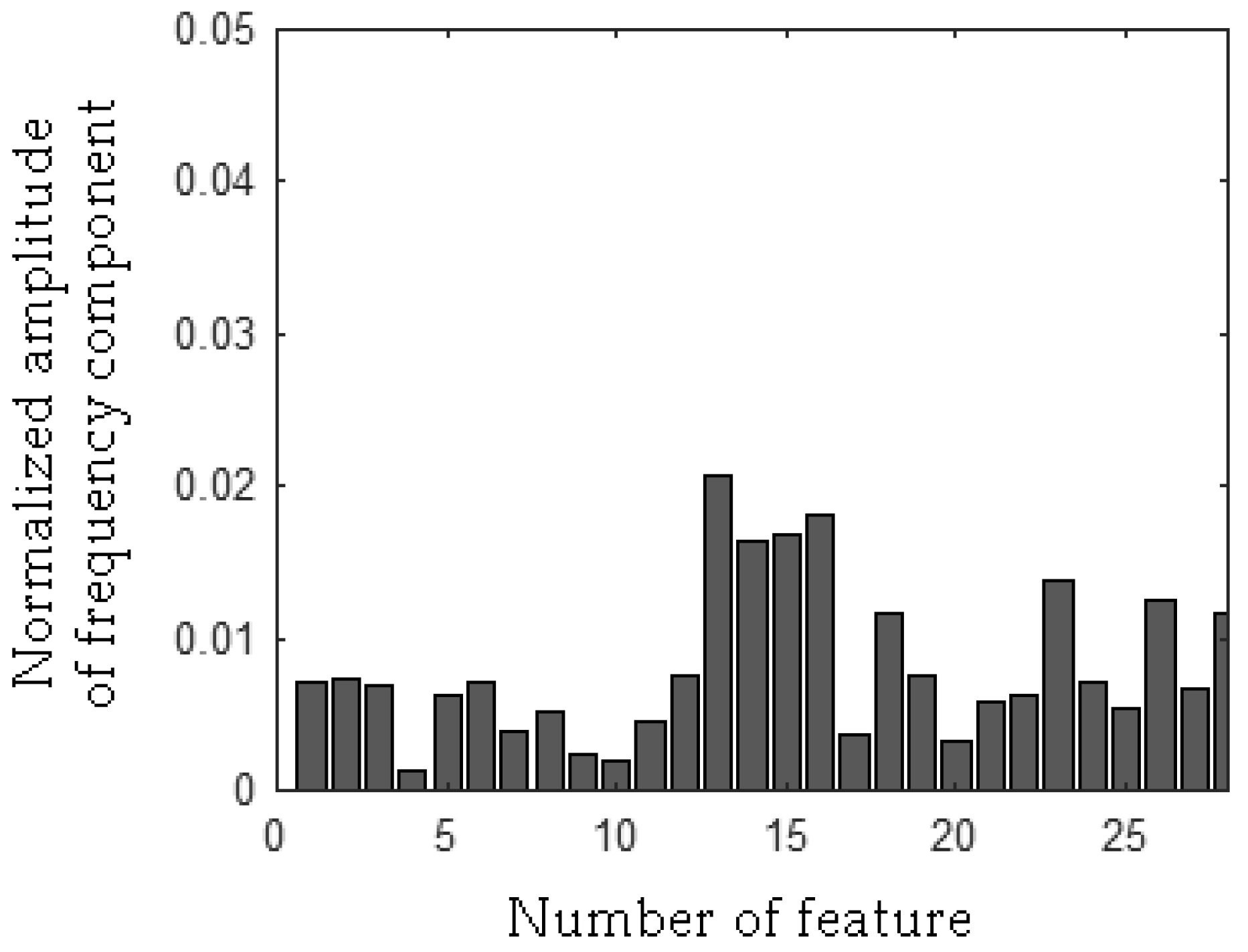
| Value of Feature | |||
|---|---|---|---|
| 0.007080 | 0.007388 | 0.006834 | 0.001410 |
| 0.006244 | 0.007172 | 0.003946 | 0.005266 |
| 0.002335 | 0.002029 | 0.004501 | 0.007593 |
| 0.020768 | 0.016296 | 0.016799 | 0.018125 |
| 0.003584 | 0.011559 | 0.007451 | 0.003169 |
| 0.007080 | 0.007388 | 0.006834 | 0.001410 |
| 0.006244 | 0.007172 | 0.003946 | 0.005266 |
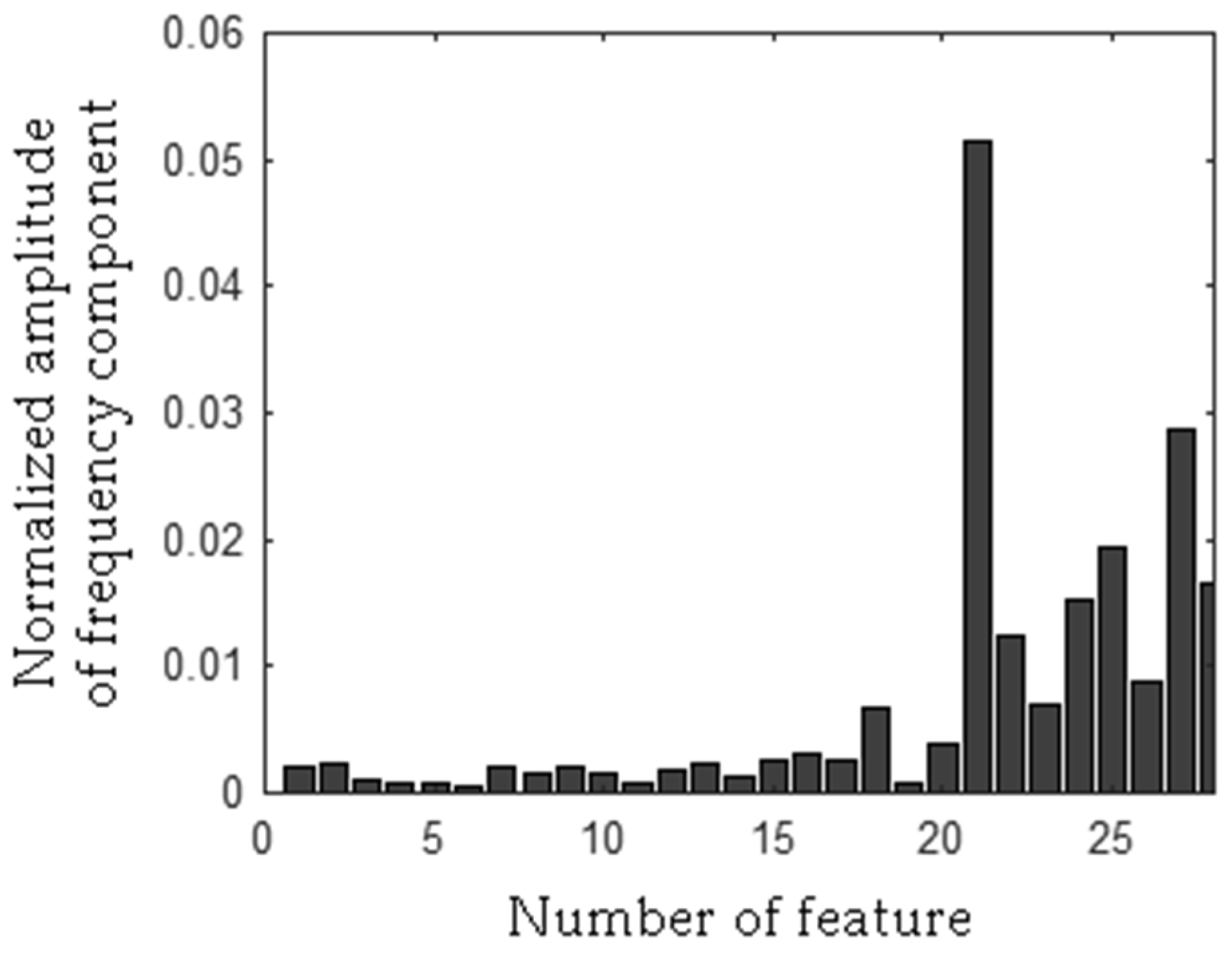
| Value of Feature | |||
|---|---|---|---|
| 0.002066 | 0.002245 | 0.001124 | 0.000820 |
| 0.000845 | 0.000655 | 0.002080 | 0.001540 |
| 0.002178 | 0.001563 | 0.000810 | 0.001933 |
| 0.002259 | 0.001234 | 0.002635 | 0.003116 |
| 0.002729 | 0.006634 | 0.000739 | 0.004000 |
| 0.051576 | 0.012309 | 0.007059 | 0.015156 |
| 0.019388 | 0.008816 | 0.028623 | 0.016604 |
| Type of Acoustic Signal | ERCM [%] |
|---|---|
| Healthy CM | 90 |
| CM with broken rotor coil | 87 |
| CM with shorted stator coils | 94 |
| CM with broken tooth on sprocket | 100 |
| CM with damaged gear train | 100 |
| TERCM [%] | |
| 94.2 |
| Type of Acoustic Signal | ERCM [%] |
|---|---|
| Healthy CM | 89 |
| CM with broken rotor coil | 91 |
| CM with shorted stator coils | 93 |
| CM with broken tooth on sprocket | 100 |
| CM with damaged gear train | 100 |
| TERCM [%] | |
| 94.6 |
| Type of Acoustic Signal | ERCM [%] |
|---|---|
| Healthy CM | 87 |
| CM with broken rotor coil | 86 |
| CM with shorted stator coils | 81 |
| CM with broken tooth on sprocket | 90 |
| CM with damaged gear train | 98 |
| TERCM [%] | |
| 88.4 |
| Type of Acoustic Signal | ERCM [%] |
|---|---|
| Healthy CM | 85 |
| CM with broken rotor coil | 88 |
| CM with shorted stator coils | 82 |
| CM with broken tooth on sprocket | 91 |
| CM with damaged gear train | 99 |
| TERCM [%] | |
| 89 |
© 2018 by the author. Licensee MDPI, Basel, Switzerland. This article is an open access article distributed under the terms and conditions of the Creative Commons Attribution (CC BY) license (http://creativecommons.org/licenses/by/4.0/).
Share and Cite
Glowacz, A. Acoustic-Based Fault Diagnosis of Commutator Motor. Electronics 2018, 7, 299. https://doi.org/10.3390/electronics7110299
Glowacz A. Acoustic-Based Fault Diagnosis of Commutator Motor. Electronics. 2018; 7(11):299. https://doi.org/10.3390/electronics7110299
Chicago/Turabian StyleGlowacz, Adam. 2018. "Acoustic-Based Fault Diagnosis of Commutator Motor" Electronics 7, no. 11: 299. https://doi.org/10.3390/electronics7110299
APA StyleGlowacz, A. (2018). Acoustic-Based Fault Diagnosis of Commutator Motor. Electronics, 7(11), 299. https://doi.org/10.3390/electronics7110299