Correction of the Unobtrusive ECG Using System Identification

Abstract

Unobtrusively acquired electrocardiograms (ECG) could substantially improve the comfort of patients. However, such ECGs are not used in clinical practice because (among other reasons) signal deformations impede correct diagnosis of the ECG. Here, methods are proposed for correction of the unobtrusive ECG, based on system identification. Knowing the reference ECG, models were developed to correct the unobtrusively acquired ECG. A finite impulse response (FIR) model, a state space model and an autoregressive model were developed. The models were trained and evaluated on the Goldberger leads recorded from an ECG T-shirt with dry electrodes, and from a gold standard ECG. It was found that the FIR model corrects the unobtrusive ECG with good agreement (${\rho }_{\mathrm{aVR}}$ = 0.84 ± 0.10, ${\rho }_{\mathrm{aVL}}$ = 0.65 ± 0.24, ${\rho }_{\mathrm{aVF}}$ = 0.88 ± 0.04), while the other models do not yield significant improvements, or become unstable. The R-peaks were also accurately corrected by the FIR model (${\mathrm{MSE}}_{\mathrm{aVR}}$ = 0.10 ± 0.10, ${\mathrm{MSE}}_{\mathrm{aVL}}$ = 0.14 ± 0.27, ${\mathrm{MSE}}_{\mathrm{aVF}}$ = 0.03 ± 0.02). To conclude, the proposed FIR method succeeded in significantly correcting the unobtrusive ECG signal.

1. Introduction

The electrocardiogram (ECG) is one of the standard clinical methods of diagnosis for cardiac-related diseases. By means of the ECG, the electrical activity of the heart is recorded and analyzed. This technology is inexpensive, easy to use and clinically established. The main drawback of the ECG is the use of adhesive electrodes that can provoke allergic reactions, especially if applied during a relatively long period. Another issue is the reduced comfort for patients, mainly due to the cables attached to the electrodes.

To overcome these issues, various unobtrusive ECG systems (uECG) have been developed. One realization method is capacitive ECG (cECG), which has been built into everyday objects such as chairs [1,2], car seats [3], beds [4,5,6,7] and clothing [8]. The principle is to use ECG electrodes incorporated in these objects that do not require conductive contact to the human body, but acquire the physiological surface potentials with capacitive coupling. Similar unobtrusive systems are dry ECGs; these have conductive contact to the skin but do not use any electrolyte gel or adhesive material [9,10,11,12]. However, the uECG requires a more complicated electronic setup [13,14]. In many cases, an operational amplifier is used as a buffer located directly at the electrode that drives the electrode cable and reduces interference (active electrode). Nevertheless, these systems have their drawbacks, e.g., they are especially prone to movement artifacts. So far, uECG are foremost used in laboratory settings or clinical studies.

For the cECG in particular, several hardware-based approaches have been proposed to improve the quality, but they have also increased the complexity of the circuits [14,15,16]. Furthermore, the morphology of the cECG differs slightly from that of the standard ECG, which is important for clinical diagnosis. When comparing the shape of the ECGs, a study using a cECG chair showed that some features could be reliably extracted, including the heart rate and QRS duration, as well as QT and PQ length. However, other features of the ECG were distorted, i.e., (1) depression of the ST segment; (2) flattening of the R-peak; (3) depression of the S wave below the equipotential line; (4) a rounding of the QRS complex [17,18].

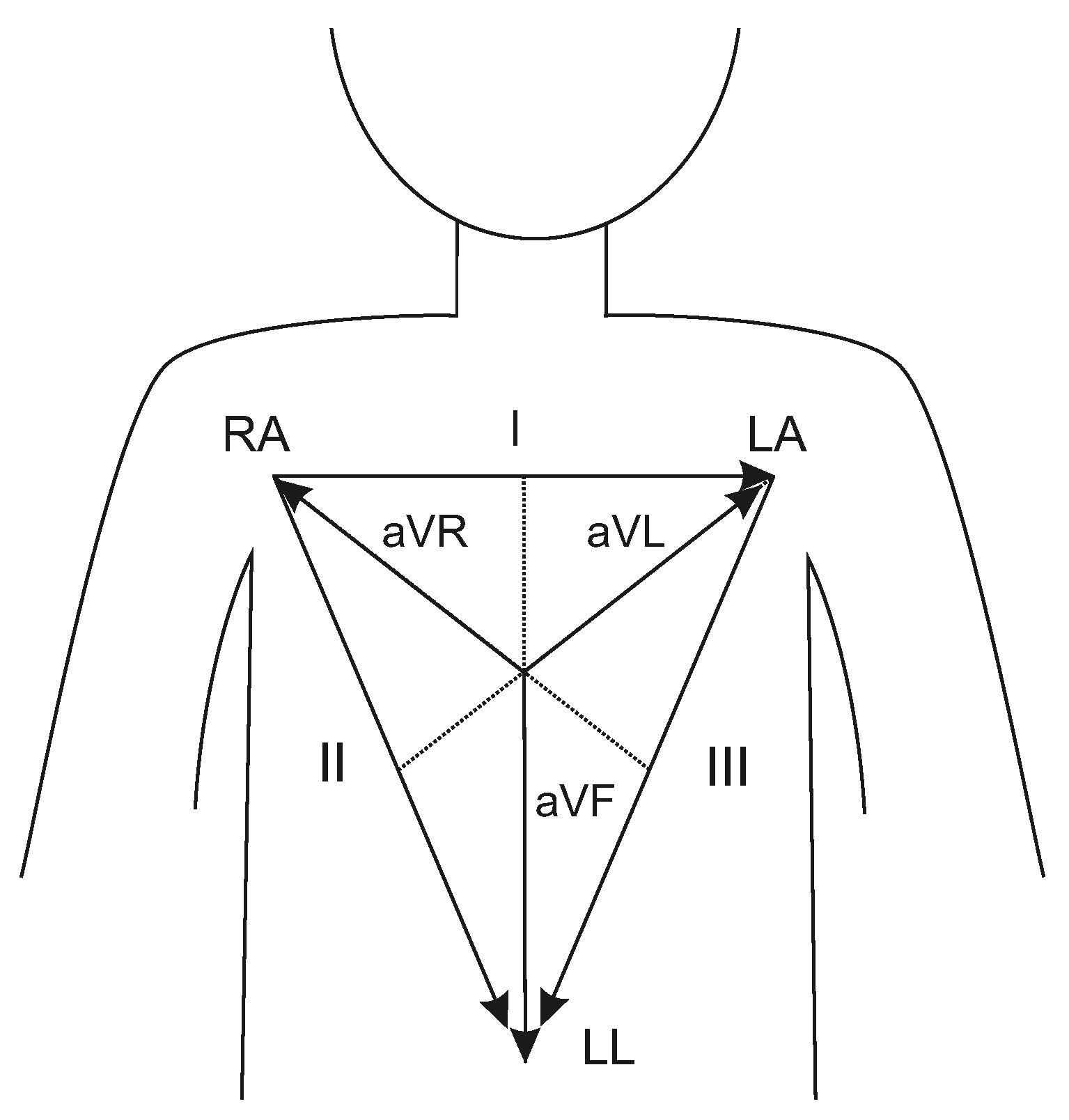
Previously, our group described the development of a dry 12-lead ECG T-shirt with active electrodes [19]. It was found that the accuracy of the system related to extracting the beat-to-beat intervals was very high, whereas some morphological features of the ECG waves (especially of the T wave) were not in agreement with the reference ECG [19].

The aim of this study is to present different models and transfer functions to correct and compensate a uECG for deformations that arise due to the recording setup. After a short calibration phase using a uECG (dry-contact) and a reference ECG, models are trained that can be applied for correction of the subsequent uECG acquisition. The approach performs system identification using an finite impulse response (FIR) model, a state space model (SSM) and an autoregressive with exogenous terms (ARX).

Section 2 introduces the study, presents an equivalent system model for a uECG, and describes different methods for system identification. Section 3 gives the results, Section 4 presents the discussion and Section 5 gives the conclusions.

2. Materials and Methods

2.1. Study

A study was conducted with seven healthy participants (4 male, 3 female) and utilizing data from three healthy male volunteers participating in [19]. All subjects gave their informed consent for inclusion before they participated in the study. The study was conducted in accordance with the Declaration of Helsinki, and the protocol was approved by the Ethics Committee of RWTH Aachen University (Reference code: EK 283/17). The volunteers were asked to wear the dry 12-lead ECG T-shirt [19] and a reference Holter ECG BT12 (Corscience, Erlangen, Germany) while sitting still and relaxed in front of their desks. The dry ECG electrodes were located on the interior of the T-shirt. The three Goldberger leads were recorded (the duration of each recording was 5 min). The data were post-processed on a PC with an Intel Core i5-2500 CPU @ 3.30 GHz (Intel Corporation, Santa Clara, CA, USA) and 8 GB RAM. Two of the new recordings were discarded because of excessive noise (two male participants). The data needed to be clean in order to conduct training for the models; artifacts were rejected afterwards.

Table 1. Recordings used for the present study.

Subject ID	Gender	Duration	Noise
1	male	296.52 s	-
2	male	297.56 s	-
3	male	297.56 s	-
4	female	282.90 s	50 Hz
5	female	266.17 s	50 Hz
6	female	299.20 s	50 Hz
7	male	298.85 s	50 Hz
8	male	292.99 s	50 Hz

lists the recordings that were used for this paper.

For the ECG, the differential leads are recorded and not the surface potential at each electrode. Since the equations for the ECG leads are linearly dependent, it is not possible to determine the surface potential directly at each electrode. The electrodes are denoted left arm (LA), right arm (RA) and left leg (LL), see Figure 1. The Einthoven leads are most frequently selected: I = LA − RA, II = LL − RA, III = LL − LA.

For the present study, the unipolar Goldberger leads were chosen (augmented voltage right (aVR), augmented voltage left (aVL) and augmented voltage foot (aVF)). The leads aVR = RA − 1/2(LA + LL), aVL = LA − 1/2(RA + LL) and aVF = LL − 1/2(RA + LA) were selected, because each one can be attributed to a different limb [20].

2.2. Pre-Processing of the ECG Data

Data pre-processing was conducted prior to system identification (Figure 2).

First, the raw data from the T-shirt ECG and the reference device were synchronized, as reported in [19]. The Goldberger leads aVL, aVF and aVR were selected for system identification. The data from each channel of the reference and uECG were filtered with a digital 4th-order high-pass zero-phase filter at 0.5 Hz to remove the DC component. The optimal frequency boundaries within which the ECG should not be distorted are between 0.5 and 40 Hz. After filtering, the data were resampled from 500 Hz to a lower resolution of 200 Hz with the MATLAB (The Mathworks, Nattick, MA, USA) resample function, since only frequency components below 100 Hz were of interest. Subsequently, artifacts with large amplitudes were removed manually, because their presence would impede system identification, see Figure 3b. Also, because some of the experiments contained strong 50 Hz line noise (Figure 3a), a subtraction procedure was applied which removes power line interference but does not alter the ECG [21,22].

2.3. Blind System Identification

The approach is to use methods of black or grey box system identification. The assumption is that the underlying system is unknown and only the input and output are available, see Figure 4. The first method is to determine a finite impulse response (FIR) filter of Nth order

$$y[n]=\sum _{i=0}^N{b}_i·x[n-i]$$

(1)

with input x[n], output y[n] and $b_i$ filter coefficients. The input is the uECG and the output the estimated reference ECG. FIR filters have the advantage that they are always stable and are simple to realize. The feasibility of using an FIR filter to estimate the reference ECG from the cECG was demonstrated in [23,24]. The presented deconvolution method in particular made use of the fact that the convolution operation in the time domain becomes a simple multiplication in the frequency domain. It was demonstrated that the deconvolution of three capacitive ECG channels led to an improved estimate of the underlying reference ECG. The results of the root-mean-square error and the Pearson correlation coefficient indicated an improvement compared to the single capacitive channels. However, the cECG leads were not recorded according to a known electrode placement system. Therefore, there was no correspondence between the reference ECG and the cECG sites RA, LA and LL, see Figure 1. In the present case, simultaneously recorded data of two devices were available from the same ECG sites, allowing a direct comparison. Since the results of the previous attempts to use deconvolution for system identification were promising, the approach of using an FIR filter was followed for this work.

The training data were used as an input to the MATLAB System Identification toolbox (The Mathworks, Nattick, MA, USA) graphical user interface. For this study, the models with the highest accuracy were selected. In addition to the FIR model, two other models were chosen for system identification: (1) a state space model (SSM); and (2) an autoregressive (AR) or autoregressive with exogenous terms (ARX) model. The structure of an SSM is as follows:

$$\stackrel{·}{x}(t)=Ax(t)+Bu(t)+Ke(t)$$

(2)

$$y(t)=Cx(t)+Du(t)+e(t)$$

(3)

with u(t) input, y(t) output, A, B, C and D state matrix, e(t) noise and K noise matrix.

The structure of an ARX model is as follows:

$$y(t)+\sum _{i=1}^{n_a}{a}_{i}y(t-i)=\sum _{i=n_k}^{n_b}{b}_{i}u(t-i)+e(t)$$

(4)

with u(k) input, y(k) output, $n_k$ system delay, $n_a$ AR order, $n_b$ X order and e(k) noise.

2.4. Training and Testing Technique

The recordings were divided into training and test data; the training data (5 heart beats) were used for the estimations for each subject, the remainder was test data. Input and output data were digitally filtered and aligned around zero for each channel separately.

The training phase was as follows:

• Short, clean segments of the data were manually selected as training data (5 QRS complexes) for each subject and per channel (aVR, aVL, aVF).
• The locations of the R-peaks of the uECG and reference ECG were aligned manually to receive matching input and output data.
• System identification was performed to obtain FIR, SSM and ARX models, see Figure 5a.

For the test or validation phase, test data were used as an input to the identified models and transfer functions, see Figure 5b. The overall concept for uECG correction is shown in Figure 5.

Additionally, for the FIR filters, leave-one-out cross-validation was conducted for each lead separately. For each round of cross-validation one dataset (one subject) was the test set and the other datasets (all other subjects) were used as training set. Therefore, the filters were trained on the data of all other subjects and then applied to the data of the remaining subject.

3. Results

First, the results of the training phase are presented in Section 3.1. Then, the resulting model orders for blind system identification are presented in Section 3.1.1, see Figure 4. General observations during the training phase are presented in Section 3.1.2. In Section 3.2, the results of system identification on test data are shown:

• Time-based analysis
• ECG morphology analysis
• Frequency analysis.

3.1. Training Phase

3.1.1. Estimation of Blind System Identification Orders

For system identification, each channel was taken separately and used for estimation in a single input, single output structure. First, the model orders were determined by the MATLAB System Identification toolbox. The automatically selected filter length for FIR was N = 46, using the MATLAB impulseest function. The SSM was chosen as a 4th order model with the MATLAB n4sid function. Further, the ARX model was ${\mathrm{n}}_a$ = 4, ${\mathrm{n}}_b=4$, ${\mathrm{n}}_k=0$ with the MATLAB arx function. These fixed filter and model orders were chosen for this study.

3.1.2. Training Outcomes

During the training phase, different qualities for the estimations were observed on visual inspection (Figure 6): examples of different qualities of estimation results are shown. The different errors are marked in the graphs. In (b), a dent in the Q wave and an overshoot of the T wave occurred in the estimation of aVR. In (3) the P wave was deformed, the Q wave was flattened, the S wave had a dent, and the T wave had an overshoot.

3.2. Test Phase

3.2.1. Time-Based Analysis

Evaluation of the filters was conducted on the test (or validation) data.

Table 2. Correlation coefficient of estimation on validation data, compared to uECG.

Subject	aVR					aVL					aVF
	uECG	FIR	SSM	ARX		uECG	FIR	SSM	ARX		uECG	FIR	SSM	ARX
1	0.65	0.88	0.72	x		0.87	0.90	0.80	0.89		0.86	0.86	0.83	0.84
2	0.28	0.84	0.84	0.83		0.09	0.65	0.36	0.35		0.27	0.86	0.82	0.83
3	0.53	0.62	0.50	0.48		0.22	0.22	x	−0.05		0.87	0.86	x	x
4	0.75	0.89	x	0.73		0.54	0.63	0.09	0.31		0.45	0.91	0.77	0.84
5	0.52	0.79	0.37	x		∗	∗	∗	∗		0.47	0.81	0.15	−0.46
6	0.90	0.87	0.53	0.65		∗	∗	∗	∗		0.92	0.92	0.86	0.91
7	0.94	0.94	0.80	0.93		0.62	0.83	0.73	0.65		0.94	0.95	0.72	0.95
8	0.51	0.91	0.76	0.91		0.15	0.69	0.64	0.57		0.54	0.90	0.90	0.90
mean(abs)	0.64	0.84	0.64	0.65		0.41	0.65	0.52	0.47		0.67	0.88	0.72	0.82
std(abs)	0.22	0.10	0.18	0.33		0.31	0.24	0.30	0.29		0.26	0.04	0.26	0.16

∗ Recording excluded, x instability.

shows the correlations $\rho$ between the reference ECG channels and the other ECG modalities, while the uECG served as a benchmark. Some of the models proved to be unstable during estimation and are indicated with an ’x’ in Table 2. The mean was calculated from the absolute values, ignoring the missing values; the same was done for the standard deviation. The modality with the highest correlation coefficient is highlighted for each subject and for each channel. The best correlation was achieved by the stable FIR filter for all channels (${\rho }_{\mathrm{aVR}}$ = 0.84 ± 0.10, ${\rho }_{\mathrm{aVL}}$ = 0.65 ± 0.24, ${\rho }_{\mathrm{aVF}}$ = 0.88 ± 0.04) compared to the uECG (${\rho }_{\mathrm{aVR}}$ = 0.64 ± 0.21, ${\rho }_{\mathrm{aVL}}$ = 0.41 ± 0.31, ${\rho }_{\mathrm{aVF}}$ = 0.67 ± 0.26) with an improvement by 0.2 for aVR, 0.24 for aVL and 0.21 for aVF. The other modalities (SSM and ARX) performed similarly to the uECG (${\rho }_{\mathrm{aVR}}$ = 0.65 ± 0.01, ${\rho }_{\mathrm{aVL}}$ = 0.50 ± 0.04, ${\rho }_{\mathrm{aVF}}$ = 0.77 ± 0.07). For the aVL lead, poor estimation results were acquired in all experiments.

Additionally, leave-one-out cross-validation was performed with the FIR filters.

Table 3. Leave-one-out correlation coefficients for finite impulse response (FIR), compared to uECG.

Subject	aVR			aVL			aVF
	uECG	FIR		uECG	FIR		uECG	FIR
1	0.66	0.79		0.87	0.71		0.86	0.85
2	0.28	0.24		0.09	0.12		0.27	0.33
3	0.53	0.64		0.22	0.21		0.87	0.72
4	0.76	0.79		0.54	0.51		0.45	0.59
5	0.52	0.41		∗	∗		0.47	0.43
6	0.90	0.88		∗	∗		0.92	0.89
7	0.94	0.86		0.62	0.81		0.94	0.82
8	0.51	0.45		0.15	0.13		0.54	0.56
mean(abs)	0.64	0.63		0.31	0.31		0.67	0.65
std(abs)	0.22	0.24		0.32	0.32		0.26	0.20

∗ Recording excluded.

shows the results of the cross-validation. Using the filters trained on other subjects, no discernible improvement was achieved. Overall, the correlation coefficients were in the same range as for the uECG.

3.2.2. ECG Morphology Analysis

One of the morphological differences between the uECG and the reference ECG is R-peak flattening. In

Table 4. Mean square error for the amplitude deviation of the R-peaks.

Subject	aVR					aVL					aVF
	uECG	FIR	SSM	ARX		uECG	FIR	SSM	ARX		uECG	FIR	SSM	ARX
1	1.48	0.14	0.04	x		1.29	0.68	0.49	0.77		0.63	0.02	0.17	0.05
2	2.21	0.10	0.06	0.14		0.14	-	-	-		0.09	0.05	0.04	0.04
3	9.10	0.32	0.68	0.98		4.36	0.12	x	0.01		1.53	0.07	x	x
4	2.15	0.06	x	0.09		-	0.08	-	-		0.84	0.02	0.06	0.04
5	1.04	0.08	0.75	x		∗	∗	∗	∗		0.44	0.04	-	-
6	0.69	0.01	0.48	0.15		∗	∗	∗	∗		0.27	0.01	0.01	0.01
7	0.25	0.02	0.05	0.03		0.03	0.00	0.00	0.00		0.08	0.00	0.01	0.00
8	1.08	0.05	0.14	0.05		-	-	-	-		0.18	0.01	0.01	0.01
mean(abs)	2.25	0.10	0.28	0.18		0.97	0.14	0.08	0.13		0.51	0.03	0.04	0.02
std(abs)	2.85	0.10	0.31	0.33		1.73	0.27	0.20	0.31		0.49	0.02	0.06	0.02

∗ Recording excluded, x instability, - segmentation fail.

the deviation of the R-peaks is evaluated using the mean square error measure (MSE) in arbitrary units (a.u.). The ECG waves were extracted using the algorithm from [19]. The flattening of the R-peaks for the uECG can be observed, especially in aVR (${\mathrm{MSE}}_{\mathrm{aVR}}$ = 2.45 ± 2.85, ${\mathrm{MSE}}_{\mathrm{aVL}}$ = 0.97 ± 1.73, ${\mathrm{MSE}}_{\mathrm{aVF}}$ = 0.51 ± 0.49). With only one exception, an overall improvement occurred for the height of the R-peak (except for the system model estimation in aVF). Some experiments did not result in reasonable R-peak estimations when, e.g., the model was unstable (MSE infinite). Additionally, in some cases the segmentation failed because of irregular shapes of the ECG, e.g., if the T wave was higher than the R peak. The FIR estimation performed exceptionally well in estimating the correct R-peaks (${\mathrm{MSE}}_{\mathrm{aVR}}$ = 0.10 ± 0.10, ${\mathrm{MSE}}_{\mathrm{aVL}}$ = 0.14 ± 0.27, ${\mathrm{MSE}}_{\mathrm{aVF}}$ = 0.03 ± 0.02).

For the other waves (P, Q, S and T), the estimations did not significantly improve the amplitude of the waves compared to the uECG, see Appendix A

Table A1. Mean squared error for the amplitude deviation of the P waves.

Subject	aVR					aVL					aVF
	uECG	FIR	SSM	ARX		uECG	FIR	SSM	ARX		uECG	FIR	SSM	ARX
1	0.01	0.00	0.02	x		0.01	0.00	0.00	0.01		0.00	0.01	0.00	0.03
2	0.02	0.04	0.04	0.04		0.01	-	-	-		0.03	0.01	0.02	0.02
3	0.05	0.24	0.49	0.61		0.06	0.01	x	0.00		0.05	0.06	x	x
4	0.02	0.01	x	0.06		-	0.00	-	-		0.02	0.01	0.06	0.03
5	0.01	0.02	0.03	x		∗	∗	∗	∗		0.02	0.02	-	-
6	0.00	0.01	0.03	0.03		∗	∗	∗	∗		0.00	0.00	0.02	0.00
7	0.00	0.00	0.01	0.00		0.00	0.00	0.00	0.00		0.00	0.00	0.01	0.00
8	0.01	0.02	0.03	0.02		-	-	-	-		0.00	0.00	0.00	0.00
mean(abs)	0.02	0.04	0.09	0.13		0.02	0.00	0.00	0.00		0.02	0.01	0.02	0.01
std(abs)	0.02	0.08	0.17	0.24		0.03	0.00	0.00	0.00		0.02	0.02	0.02	0.01

∗ Recording excluded, x instability, - segmentation fail.

,

Table A2. Mean squared error for the amplitude deviation of the Q waves.

Subject	aVR					aVL					aVF
	uECG	FIR	SSM	ARX		uECG	FIR	SSM	ARX		uECG	FIR	SSM	ARX
1	0.19	0.00	0.05	x		0.10	0.09	0.02	0.06		0.19	0.05	0.14	0.05
2	0.09	0.02	0.03	0.03		0.05	-	-	-		0.03	0.01	0.03	0.02
3	0.11	0.40	0.61	0.70		0.09	0.01	x	0.00		0.07	0.07	x	x
4	0.15	0.06	x	0.09		-	0.00	-	-		0.11	0.02	0.06	0.04
5	0.01	0.02	0.07	x		∗	∗	∗	∗		0.03	0.02	-	-
6	0.01	0.01	0.03	0.00		∗	∗	∗	∗		0.00	0.00	0.02	0.00
7	0.02	0.00	0.01	0.00		0.00	0.00	0.00	0.00		0.00	0.00	0.03	0.00
8	0.01	0.02	0.18	0.02		-	-	-	-		0.00	0.01	0.01	0.00
mean(abs)	0.07	0.07	0.14	0.14		0.06	0.02	0.01	0.02		0.05	0.02	0.05	0.02
std(abs)	0.07	0.14	0.21	0.28		0.04	0.04	0.02	0.03		0.07	0.02	0.05	0.02

∗ Recording excluded, x instability, - segmentation fail.

,

Table A3. Mean squared error for the amplitude deviation of the S waves.

Subject	aVR					aVL					aVF
	uECG	FIR	SSM	ARX		uECG	FIR	SSM	ARX		uECG	FIR	SSM	ARX
1	0.02	0.01	0.03	x		0.38	0.25	0.35	0.24		0.01	0.01	0.07	0.02
2	0.01	0.06	0.06	0.03		0.04	-	-	-		0.03	0.02	0.03	0.03
3	0.20	0.46	0.79	1.20		0.09	0.02	x	0.03		0.11	0.07	x	x
4	0.01	0.03	x	0.08		-	0.02	-	-		0.02	0.02	0.06	0.03
5	0.09	0.05	0.04	x		∗	∗	∗	∗		0.10	0.02	-	-
6	0.06	0.01	0.03	0.15		∗	∗	∗	∗		0.03	0.00	0.01	0.00
7	0.06	0.01	0.01	0.04		0.00	0.00	0.00	0.00		0.06	0.00	0.03	0.00
8	0.01	0.08	0.00	0.05		-	-	-	-		0.00	0.01	0.01	0.00
mean(abs)	0.06	0.09	0.14	0.26		0.13	0.07	0.17	0.09		0.04	0.02	0.03	0.01
std(abs)	0.07	0.15	0.29	0.46		0.17	0.12	0.24	0.13		0.04	0.02	0.02	0.01

∗ Recording excluded, x instability, - segmentation fail.

and

Table A4. Mean squared error for the amplitude deviation of the T waves.

Subject	aVR					aVL					aVF
	uECG	FIR	SSM	ARX		uECG	FIR	SSM	ARX		uECG	FIR	SSM	ARX
1	0.01	0.01	0.17	x		0.02	0.03	0.00	0.01		0.00	0.01	0.01	0.02
2	0.04	0.13	0.19	0.17		0.03	-	-	-		0.05	0.03	0.05	0.05
3	0.06	0.42	1.20	1.63		0.35	0.04	x	0.00		0.05	0.04	x	x
4	0.01	0.04	x	0.11		-	0.02	-	-		0.02	0.02	0.05	0.05
5	0.02	0.02	0.16	x		∗	∗	∗	∗		0.02	0.03	-	-
6	0.04	0.01	0.07	0.01		∗	∗	∗	∗		0.01	0.00	0.01	0.01
7	0.03	0.00	0.04	0.01		0.00	0.00	0.00	0.00		0.02	0.00	0.03	0.00
8	0.06	0.02	0.00	0.03		-	-	-	-		0.08	0.03	0.03	0.04
mean(abs)	0.03	0.08	0.26	0.33		0.10	0.02	0.00	0.01		0.03	0.02	0.03	0.03
std(abs)	0.02	0.14	0.42	0.64		0.17	0.02	0.00	0.01		0.03	0.02	0.02	0.02

∗ Recording excluded, x instability, - segmentation fail.

. Lastly, for SSM and ARX, no notable improvements were observed compared with the uECG.

3.2.3. Frequency Analysis

The spectral properties of the data were also analyzed. In Figure 7, the power spectrum of the uECG is compared to the reference ECG and the estimations. In this example, the FIR filter was used (subject 1, aVR). The power spectra of the estimations FIR, and ARX resemble the power spectrum (0–40 Hz) of the reference ECG (Figure 7).

The coherence estimate and the cross-spectrum phase of the ECGs were also analyzed (Figure 8). In Figure 8, the coherence estimate $C_{xy}$ is shown with

$$C_{xy}(\omega )=\frac{|P_{xy}{|}^2(\omega )}{P_{xx}(\omega )P_{yy}(\omega )},$$

(5)

with $P_{xx}$, $P_{yy}$ power spectral densities of the signals x and y, and the cross-power spectral density P_xy. Coherence close to one indicates equality at a certain frequency of two given signals, while a value close to zero indicates inequality. In our case, for all subjects the resulting coherence estimates were very similar for the reference and uECG, as well as for the reference and estimation ECG.

However, the cross-spectrum phase indicated some additional information: If the coherence has a large value, the phase of the cross-spectrum can be determined, thus identifying phase lags. Although the coherence estimate was not significant, the cross-spectrum phase pinpointed the differences. For the example presented in Figure 8, the cross-spectrum phase of the estimated ECG (FIR filter) with the reference had lower values than the uECG with the reference.

Table 5. Mean of absolute cross-spectrum phase values (0–40 Hz).

Subject	aVR					aVL					aVF
	uECG	FIR	SSM	ARX		uECG	FIR	SSM	ARX		uECG	FIR	SSM	ARX
1	29.27	17.68	37.58	89.78		19.42	14.35	43.54	17.09		19.30	12.73	30.99	13.43
2	108.18	19.87	16.35	16.73		85.07	21.71	44.29	41.71		107.33	13.69	13.17	13.79
3	16.44	38.54	42.46	39.29		74.50	77.89	x	86.93		13.71	19.16	x	x
4	32.10	12.78	x	13.95		50.77	27.93	55.84	52.65		87.66	9.53	10.50	9.28
5	62.94	23.97	54.01	x		∗	∗	∗	∗		63.10	19.39	66.77	76.94
6	15.61	31.03	39.44	58.62		∗	∗	∗	∗		15.62	30.79	36.57	32.52
7	28.05	18.98	54.83	32.64		54.13	38.11	59.73	41.23		23.50	14.04	47.69	17.26
8	115.77	21.75	22.83	22.86		113.09	26.94	49.55	50.64		100.78	24.38	23.05	21.83
mean(abs)	51.05	23.08	38.21	39.12		66.16	34.49	50.59	48.37		53.87	17.96	32.68	26.44
std(abs)	40.38	8.17	14.49	27.04		32.24	22.65	7.10	22.73		40.50	6.98	19.88	23.51

∗ Recording excluded, x instability.

shows the mean absolute of the cross-spectrum phase values. Lower values indicate lower phase lags between the reference ECG and the other ECGs. The lowest values were achieved with the FIR estimations.

4. Discussion

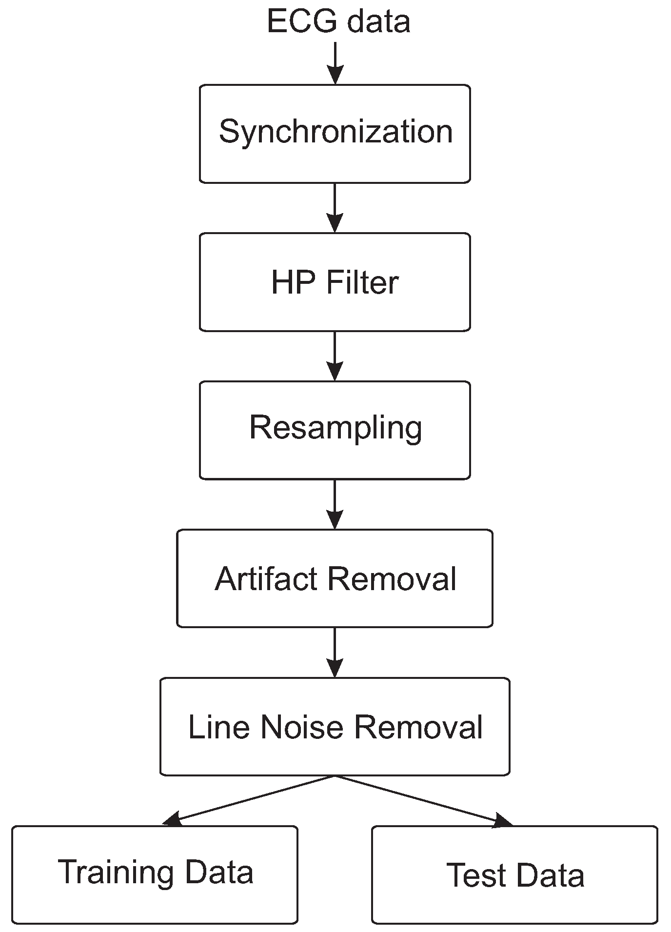
This paper presents different approaches to determine a model usable for correction and compensation of capacitive coupling occurring in uECG signals. The approach is to blindly perform system identification using an FIR model, a SSM and an ARX model. These models were trained on short excerpts of five heartbeats and were later validated on test data.

The goal was to evaluate different methods to correct deformations in a uECG using system identification. After a short calibration phase using a reference ECG and uECG, a correction method was applied to the following uECG acquisition. The models do not take into account changes in the electrode-skin interface, e.g., loss of electrode contact, but take into account the changes in ECG morphology due to the ECG acquisition method.

The use of FIR filters proved to be a feasible correction method. For each lead and each subject, an individual FIR filter was estimated. The estimated ECG was in better agreement compared to the reference ECG, which was supported by the high correlation coefficients (${\rho }_{\mathrm{aVR}}$ = 0.84 ± 0.10, ${\rho }_{\mathrm{aVL}}$ = 0.65 ± 0.24, ${\rho }_{\mathrm{aVF}}$ = 0.88 ± 0.04). The improvement of the correlation of the ECGs was consistent with our findings in [23]; analysis of the spectrum also supported this statement. Regarding morphology, the flattening of the R-peaks was successfully corrected (${\mathrm{MSE}}_{\mathrm{aVR}}$ = 0.10 ± 0.10, ${\mathrm{MSE}}_{\mathrm{aVL}}$ = 0.14 ± 0.27, ${\mathrm{MSE}}_{\mathrm{aVF}}$ = 0.03 ± 0.02). The other ECG waves (P, Q, S and T) were comparable with the uECG. To summarize: FIR filters had the best properties for correcting the uECG recordings. It is possible to tune the models by selecting different filter lengths (FIR) or model orders. We assume that the discrepancy between aVL and the other leads was probably due to an unknown acquisition error. Several sources of acquisition disturbances exist, the prominent are movement and high-frequency noise [25]. We assume that our problems were due to insufficient electrode contact to the skin, leading to more movement artifacts or baseline wander. Furthermore, the setting for the study was in an office space with computers and electronic devices that lead to high-frequency noise.

For the SSM and the ARX, in most experiments, the correlation coefficient did not indicate a better agreement with the reference ECG than with the uECG. Furthermore, a few of the estimated models were unstable for the SSM model (aVR subject 4, aVL subject 3, aVF subject 3) and the ARX model (aVR subject 1, 5; aVL subject 3, aVF subject 3). For future applications, each model needs to be checked for stability before it is used for correction. The values of the cross-spectrum indicated a slightly better agreement with the reference ECG for aVL and a much higher agreement with aVF than the uECG. In the analysis of the ECG waves, the flattening of the R-peak was corrected by both models. The MSE of the other waves indicated inconsistent results that showed no significant improvement compared with the uECG.

In future studies, additional issues of unobtrusive ECGs that are related to artifacts (based on motion or electric discharge) also need to be addressed. However, automatic correction of artifacts was not an aim of the present study; artifacts were selected and rejected manually. Meanwhile, different approaches have been proposed to remove and correct for ECG artifacts [26,27,28,29].

In the future, medical professionals should visually verify whether the corrected uECG can be used for purposes of diagnosis. Additional features of interest include: the PQ length, QRS width, ST length, and the P and T length. These features are not readily available and require more sophisticated computing or manual extraction by a medical professional. Although segmentation algorithms for ECG exist, they are reported to fail for, e.g., the capacitive ECG [30].

A short calibration procedure is necessary for the correction using the models. A recording procedure with the uECG is proposed as follows:

(1)

Simultaneous recording of the uECG and the reference ECG for 30 s.

(2)

Automated data processing:

(a)

Alignment of the uECG and the reference ECG channel data.

(b)

Performance of system identification to obtain models.

(c)

Choice of best model for uECG correction.

(3)

Removal of the reference ECG.

(4)

Long-term uECG recording using the obtained model for correction.

The short calibration phase (steps 1–3) is added to the time needed to apply a standard ECG. In step 4, either a real-time correction can be implemented in the ECG software, or an offline correction is applied afterwards. The need for calibration for each subject or even each acquisition is known in clinical practice, i.e., in EEG acquisition. Artifacts from eye movements are removed by different methods and most require calibration before each EEG recording [31]. Instead of calibration, more general models might be found, when a larger study group is available. However, individualized filters have the advantage that they correct more precisely for the given ECG setup, as demonstrated in the present leave-one-out cross-validation.

5. Conclusions

In conclusion, three different models for the correction of ECG deformations have been presented and compared. The method using an FIR filter performed particularly well. The corrected ECG curves had a significantly higher agreement with the reference ECG than the uncorrected ECG.

References

1. Lim, Y.G.; Kim, K.K.; Park, K.S. ECG measurement on a chair without conductive contact. IEEE Trans. Biomed. Eng. 2006, 53, 956–959. [Google Scholar] [PubMed]
2. Baek, H.J.; Chung, G.S.; Kim, K.K.; Park, K.S. A smart health monitoring chair for nonintrusive measurement of biological signals. IEEE Trans. Inf. Technol. Biomed. 2012, 16, 150–158. [Google Scholar] [CrossRef] [PubMed]
3. Leonhardt, S.; Aleksandrowicz, A. Non-contact ECG monitoring for automotive application. In Proceedings of the 2008 5th IEEE International Summer School and Symposium on Medical Devices and Biosensors, Hong Kong, China, 1–3 June 2008; pp. 183–185. [Google Scholar]
4. Ishijima, M. Monitoring of Electrocardiograms in Bed Without Utilizing Body Surface Electrodes. IEEE Trans. Biomed. Eng. 1993, 40, 593–594. [Google Scholar] [CrossRef] [PubMed]
5. Lim, Y.G.; Kim, K.K.; Park, K.S. ECG recording on a bed during sleep without direct skin-contact. IEEE Trans. Biomed. Eng. 2007, 54, 718–725. [Google Scholar] [CrossRef] [PubMed]
6. Wu, K.F.; Zhang, Y.T. Contactless and continuous monitoring of heart electric activities through clothes on a sleeping bed. In Proceedings of the 5th International Conference on Information Technology and Applications in Biomedicine (ITAB 2008) in Conjunction with 2nd International Symposium and Summer School on Biomedical and Health Engineering (IS3BHE 2008), Shenzhen, China, 30–31 May 2008; pp. 282–285. [Google Scholar]
7. Ueno, A.; Yama, Y. Unconstrained monitoring of ECG and respiratory variation in infants with underwear during sleep using a bed-sheet electrode unit. In Proceedings of the 30th Annual International Conference of the IEEE Engineering in Medicine and Biology Society, Vancouver, BC, Canada, 20–25 August 2008; pp. 2329–2332. [Google Scholar]
8. Chi, Y.M.; Ng, P.; Jolla, L.; Kang, E.; Kang, J.; Cauwenberghs, G. Wireless Non-contact Cardiac and Neural Monitoring. In Proceedings of the Wireless Health 2010, La Jolla, CA, USA, 4–7 October 2010. [Google Scholar]
9. Valchinov, E.S.; Pallikarakis, N.E. An active electrode for biopotential recording from small localized bio-sources. Biomed. Eng. Online 2004, 3, 25. [Google Scholar] [CrossRef] [PubMed] [Green Version]
10. Gruetzmann, A.; Hansen, S.; Müller, J. Novel dry electrodes for ECG monitoring. Physiol. Meas. 2007, 28, 1375–1390. [Google Scholar] [CrossRef] [PubMed]
11. Salvo, P.; Raedt, R.; Carrette, E.; Schaubroeck, D.; Vanfleteren, J.; Cardon, L. A 3D printed dry electrode for ECG/EEG recording. Sens. Actuators A Phys. 2012, 174, 96–102. [Google Scholar] [CrossRef]
12. Silva, M.; Catarino, A.; Carvalho, H.; Rocha, A.; Monteiro, J.; Montagna, G. Study of vital sign monitoring with textile sensors in swimming pool environment. In Proceedings of the IECON 2009 (Industrial Electronics Conference), Porto, Portugal, 3–5 November 2009; pp. 4426–4431. [Google Scholar]
13. Chi, Y.M.; Jung, T.P.; Cauwenberghs, G. Dry-contact and noncontact biopotential electrodes: Methodological review. IEEE Rev. Biomed. Eng. 2010, 3, 106–119. [Google Scholar] [CrossRef] [PubMed]
14. Sun, Y.; Yu, X. Capacitive Biopotential Measurement for Electrophysiological Signal Acquisition : A Review. IEEE Sens. J. 2016, 16, 2832–2853. [Google Scholar] [CrossRef]
15. Spinelli, E.; Haberman, M.; García, P.; Guerrero, F. A capacitive electrode with fast recovery feature. Physiol. Meas. 2012, 33, 1277. [Google Scholar] [CrossRef] [PubMed]
16. Serteyn, A.; Vullings, R.; Meftah, M.; Bergmans, J.W.M. Motion Artifacts in Capacitive ECG Measurements: Reducing the Combined Effect of DC Voltages and Capacitance Changes Using an Injection Signal. IEEE Trans. Biomed. Eng. 2015, 62, 264–273. [Google Scholar] [CrossRef] [PubMed]
17. Eilebrecht, B.; Czaplik, M.; Wartzek, T.; Schauerte, P.; Leonhardt, S. Analysis of influences on capacitive ECG measurements based on a closed loop model. In Proceedings of the 6th Meeting of the European Study Group on Cardiovascular Oscillations, Berlin, Germany, 12–14 April 2010; pp. 12–15. [Google Scholar]
18. Czaplik, M.; Eilebrecht, B.; Walocha, R.; Walter, M.; Schauerte, P.; Leonhardt, S.; Rossaint, R. The Reliability and Accuracy of a Noncontact Electrocardiograph System for Screening Purposes. Anesth. Analg. 2012, 114, 322–327. [Google Scholar] [CrossRef] [PubMed]
19. Boehm, A.; Yu, X.; Neu, W.; Leonhardt, S.; Teichmann, D. A Novel 12-Lead ECG T-Shirt with Active Electrodes. Electronics 2016, 5, 75. [Google Scholar] [CrossRef]
20. Rautaharju, P.; Rautaharju, F. Investigative Electrocardiography in Epidemiological Studies and Clinical Trials; Springer Science & Business Media: Berlin, Germany, 2007. [Google Scholar]
21. Mihov, G.S.; Dotsinsky, I.A.; Levkov, C.L. Generalised Subtraction Procedure for Removing Power-Line Interference from ECG : Case of Powerline Frequency Deviation. Annu. J. Electron. 2009, 15–19. [Google Scholar]
22. Mihov, G. Subtraction procedure for removing powerline interference from ECG: Dynamic threshold linearity criterion for interference suppression. In Proceedings of the 2011 4th IEEE International Conference on Biomedical Engineering and Informatics (BMEI 2011), Shanghai, China, 15–17 October 2011; Volume 2, pp. 858–861. [Google Scholar]
23. Böhm, A.; Antink, C.H.; Leonhardt, S.; Teichmann, D. Determining the Connection between Capacitively Coupled Electrocardiography Data and the Ground Truth. In Proceedings of the IEEE Computing in Cardiology (CinC), Nice, France, 6–9 September 2015. [Google Scholar]
24. Hoog Antink, C.; Bruser, C.; Leonhardt, S. Multimodal sensor fusion of cardiac signals via blind deconvolution: A source-filter approach. In Proceedings of the IEEE Computing in Cardiology Conference (CinC), Cambridge, MA, USA, 7–10 September 2014; pp. 805–808. [Google Scholar]
25. Blanco-Velasco, M.; Weng, B.; Barner, K.E. ECG signal denoising and baseline wander correction based on the empirical mode decomposition. Comput. Biol. Med. 2008, 38, 1–13. [Google Scholar] [CrossRef] [PubMed]
26. Yu, X.; Boehm, A.; Neu, W.; Venema, B.; Marx, N.; Leonhardt, S.; Teichmann, D. A wearable 12-lead ECG T-shirt with textile electrodes for unobtrusive long-term monitoring—Evaluation of an ongoing clinical trial. In EMBEC & NBC; Springer: Singapore, 2017; pp. 703–706. [Google Scholar]
27. Sweeney, K.; Ward, T.; McLoone, S. Artifact Removal in Physiological Signals - Practices and Possibilities. IEEE Trans. Inf. Technol. Biomed. 2012, 16, 488–500. [Google Scholar] [CrossRef] [PubMed]
28. Eilebrecht, B.; Wartzek, T.; Willkomm, J.; Schommartz, A.; Walter, M.; Leonhardt, S. Motion artifact removal from capacitive ECG measurements by means of adaptive filtering. IFMBE Proc. 2011, 37, 902–905. [Google Scholar]
29. Lee, S.M.; Kim, K.K.; Park, K.S. Wavelet approach to artifact noise removal from Capacitive coupled Electrocardiograph. In Proceedings of the 30th Annual International Conference of the IEEE Engineering in Medicine and Biology Society, Vancouver, BC, Canada, 20–25 August 2008; pp. 2944–2947. [Google Scholar]
30. Eilebrecht, B.; Henriques, J.; Rocha, T.; Walter, M.; Paredes, S.; de Carvalho, P.; Czaplik, M.; Leonhardt, S. Automatic Parameter Extraction from Capacitive ECG Measurements. Cardiovasc. Eng. Technol. 2012, 3, 319–332. [Google Scholar] [CrossRef]
31. Croft, R.J.; Barry, R.J. Removal of ocular artifact from the EEG: A review. Neurophysiol. Clin. 2000, 30, 5–19. [Google Scholar] [CrossRef]
Figure 1. Diagram of electrocardiogram (ECG) lead relationships for ECG electrodes right arm (RA), left arm (LA) and left leg (LL).
Electronics 06 00094 g001
Figure 2. Pre-processing of the raw ECG data (T-shirt ECG and reference ECG).
Electronics 06 00094 g002
Figure 3. Raw unobtrusive ECG system (uECG) excerpts: (a) line noise and baseline wander (subject 5, lead aVF); (b) artifacts (subject 8, lead aVF).
Electronics 06 00094 g003
Figure 4. System identification phase for uECG: Blind system identification with models (finite impulse response (FIR), state space model (SSM) and autoregressive with exogenous terms (ARX)).
Electronics 06 00094 g004
Figure 5. Concept for correction: (a) System identification with training data from reference ECG and uECG; (b) Application of transfer functions on uECG test data.
Electronics 06 00094 g005
Figure 6. Estimation quality for different subjects (1) (aVF subject 1, FIR); (2) (aVR, subject 2, FIR); and (3) (aVF subject 1, SSM). Deformations are highlighted.
Electronics 06 00094 g006
Figure 7. (a) ECG curves (b) Power Spectrum of uECG, reference ECG and estimated ECGs (FIR, SSM, ARX): (subject 1, aVF).
Electronics 06 00094 g007
Figure 8. Example estimation of reference ECG (a) Coherence estimate of reference vs. uECG; and reference vs. estimated ECGs (b) Cross-spectrum Phase of reference vs. uECG, and reference vs. estimated ECG: (subject 1, aVF).
Electronics 06 00094 g008