Obstacle Avoidance Based-Visual Navigation for Micro Aerial Vehicles

Abstract

This paper describes an obstacle avoidance system for low-cost Unmanned Aerial Vehicles (UAVs) using vision as the principal source of information through the monocular onboard camera. For detecting obstacles, the proposed system compares the image obtained in real time from the UAV with a database of obstacles that must be avoided. In our proposal, we include the feature point detector Speeded Up Robust Features (SURF) for fast obstacle detection and a control law to avoid them. Furthermore, our research includes a path recovery algorithm. Our method is attractive for compact MAVs in which other sensors will not be implemented. The system was tested in real time on a Micro Aerial Vehicle (MAV), to detect and avoid obstacles in an unknown controlled environment; we compared our approach with related works.

1. Introduction

Unmanned Aerial Vehicles (UAVs) are applied in several applications, like surveillance, mapping, journalism, transport, rescue, military applications and environments where a human cannot access, such as radioactive areas, toxic environments and handling of dangerous objects [1].

Kendoul [2] classified UAVs into five categories according to the size and payload: Category I: full-scale; the main features are the robustness of the physical structure and the payload that they can carry; Category II: medium-scale; they have a payload higher than 10 kg and a total weight over 30 kg; Category III: small-scale; these UAVs have a payload from 2 to 10 kg, with a total weight less than 30 kg; Category IV: mini; they have a payload of 2 kg, are electrically operated, low cost, have easy maintenance and safe operation; and Category V: Micro Air Vehicles (MAVs) have a payload lower than 100 grams and are used in navigation and detection.

Most of the commercial UAVs depend on the skill of the pilot and the robustness of the communication system. One of the problems in the teleoperation of UAVs is the loss of pilot visibility and/or the signal of the Global Positioning System (GPS); the autonomous system is an alternative for solving this issue.

The autonomous systems include motion planning, path tracking, obstacle avoidance, target detection and other areas [3]. These systems require sensing, state estimation, perception and knowledge of the situation. The perception is used to detect and avoid obstacles in real time, recognize and tracking objects and environmental mapping. There are several proposals for perception, based on vision or Laser Imaging Detection And Ranging (LiDAR) [2], but these sensors are highly expensive.

We use the Bebop drone, which is a low-cost, compact MAV. Our proposal works with a perception method based on feature points for obstacle detection and a proportional control to avoid them, using a monocular camera without depending on other sensors.

This paper is organized as follows: Section 2 shows a description of the related works. The proposed obstacle detection approach is explained in Section 3. Section 4 is focused on the modeling, controller design and the algorithm for avoiding obstacles during the fly. Experiments and results are presented in Section 5. Finally, Section 6 is destined for the conclusions and future works.

2. Related Work

Research groups on robotics have proposed different techniques for obstacle avoidance, based on sensors like LiDAR [4,5,6] and RGB-D [7,8], which show robustness to identifying obstacles; but implementing these devices in a compact MAV is difficult, expensive, and also, these consume additional electrical power. When we work with UAVs and want to implement other device onboard, we need to consider the payload that they can carry, limiting the use of any UAV. Vision systems are an alternative, because they use only the integrated camera in the aerial vehicle.

In the literature, there are several vision systems based on optical flow, like [9], where the authors propose a system for controlling ultra-light airplanes using a 1D camera and translatory optic flow that avoids obstacles and keeps distance from the ground and ceiling. Other approach are autonomous collision avoidance systems for navigation within houses or indoor environments using optical flow, micro-sensors and neural networks [10,11]. In [12], there is a simulation of a navigation system with optical flow for rotary-wing UAVs to avoid lateral and frontal collisions in a 3D urban environment. The probability distributions are a robust method for computing the structure from motion (SfM) and do not require a precise calculation of optical flow at each feature point [13].

The fundamental limitation of optical flow is when flying directly toward an obstacle, because this method is based on the flying of insects, and in the case of honeybees, they never fly in a straight line toward a target, but rather make a slight zigzag pattern. This makes it difficult to use this method for frontal obstacle avoidance [10,14].

Stereo vision [15,16] is a robust approach for obstacle detection, but is limited by the baseline, because when it narrows, this gives rise to noisy estimates. Furthermore, two cameras limit the use of any compact MAVs. Bills [17] and Çelik [18] work with perspective references to estimate the desired orientation for flying the UAV, but the vehicle can only fly in structured environments. De Croon [19] uses an appearance variation cue that works with the visual appearance of an image to estimate obstacle proximity, but depends on optical flow for achieving a higher performance.

Other techniques of vision are present in [20], which shows an image-based reactive motion planner to avoid a fast approaching obstacle, and the Dubins curve-based geometry method to developed a global path planner for a fixed-wing UAV. In [21], the authors use omnidirectional cameras that do not require the estimation of range between the two platforms to resolve the collision, but they use two vehicles to obtain the view-angle.

Furthermore, the literature presents works about path planning-based UAV obstacle avoidance, like [22], where the research shows a path planning algorithm based on 3D Dubins curves to avoid static and moving obstacles, also using the variation of the Rapidly-exploring Random Tree (RRT)-like planner. Pettersson [23] proposes an operational UAV platform to supply a 3D model of a region containing buildings and road structures and generate collision-free paths autonomously and in [24] combines D* Lite and Probabilistic Roadmaps for path planning and uses stereo vision for detecting obstacles and dynamic path updating.

In spite of the use of Scale-Invariant Feature Transform (SIFT) to recognize collisions by analyzing the change in scale and location between two images [25], it is not recommended due to the low speed.

In our proposal, we use Speeded-Up Robust Features (SURF) to detect obstacles. There are several applications of SURF, like face detection [26], target tracking [27,28], simple visual navigation [29] and some works with UAVs. One of these is [30], which uses a simple bang-bang control. Our work proposes a real-time obstacle detection algorithm based on feature points and an offline modeling of the MAV for designing a controller for fixed and mobile obstacle avoidance in an unknown controlled environment.

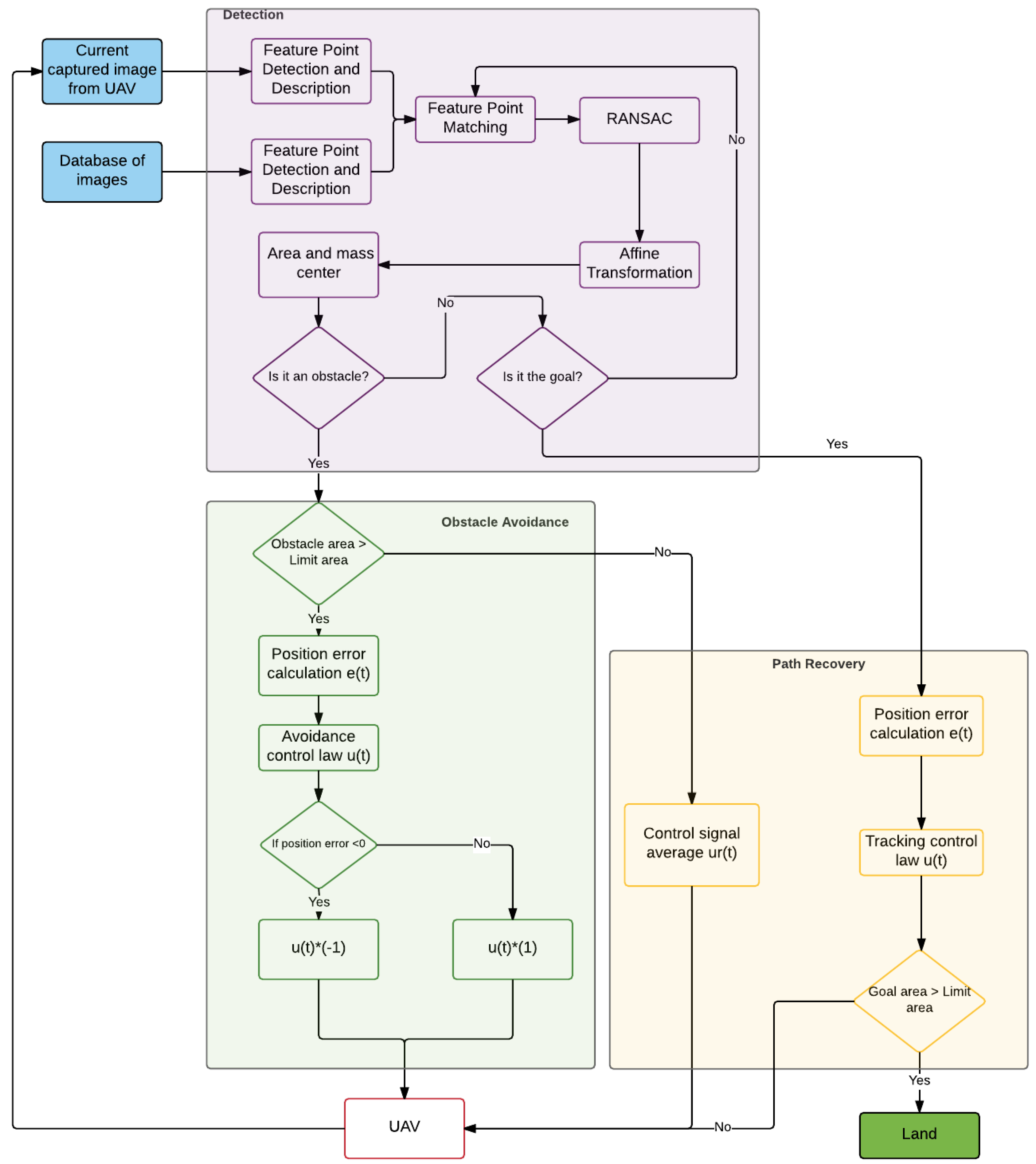
3. Obstacle Detection

In this section, we use two images; one is located in a database that contains obstacles like traffic signs, trees and a pre-designed obstacle. We use different images to demonstrate that the algorithm can detect any obstacle while it is in the database. The other image is captured with the onboard camera. In order to find correspondence between these images, feature point detection, description and matching are used. Additionally, we calculate the obstacle area and mass center to be used as a target in the controller.

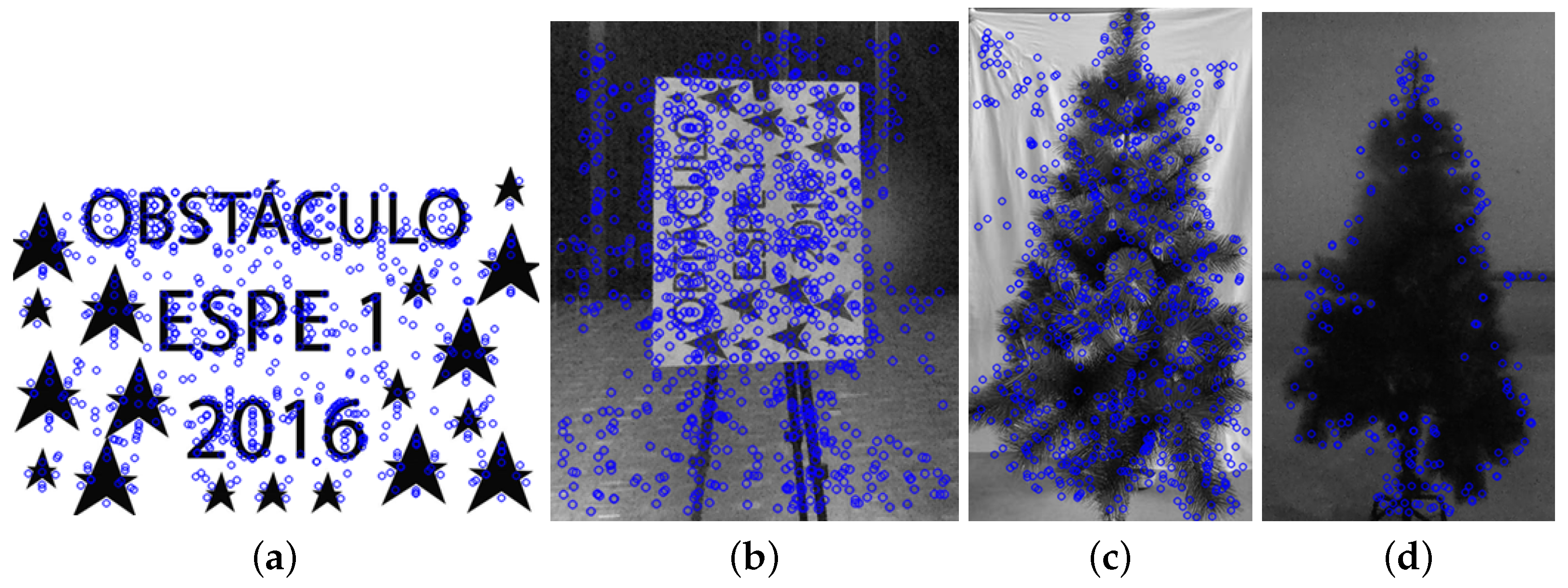
3.1. Feature Point

For feature point detection, there are several works in the literature [31,32,33], but widely-used algorithms are: Oriented Fast and Rotated Brief (ORB) [34], which is a fast binary descriptor that is rotation invariant and resistant to noise; Fast Retina Keypoint (FREAK) [35] is a method where the keypoint descriptor is inspired by the human retina; Binary Robust Invariant Scalable Keypoints (BRISK) [36] that uses a scale-space FAST-based detector with the assembly of a bit-string descriptor; Scale-Invariant Feature Transform [37], which obtains image features that are invariant to scaling, translation, rotation and partially invariant to illumination changes and affine or 3D projection; and Speeded Up Robust Feature (SURF) [38], which uses integral images to computed and compare interest points much more quickly.

In this paper, we use SURF; according to [39], the computational cost is lower without reducing robustness. The feature point can be defined by three steps: detection, description and matching.

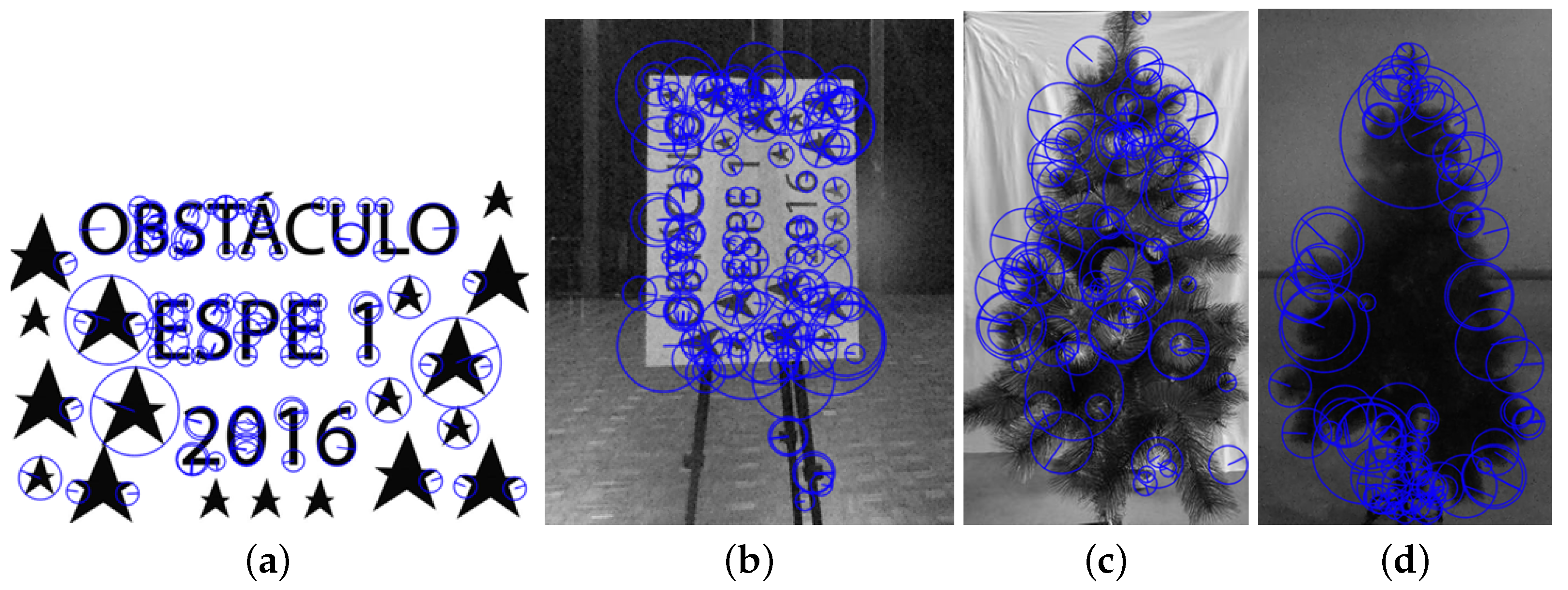
3.1.1. Feature Point Detection

The SURF algorithm for interest point detection uses a basic Hessian matrix approximation. This lends itself to the use of integral images, which reduce the computational time [38].

Integral images allow for fast computation of box-type convolution filters. The entry of an image $I_{\Sigma }\left(\mathbf{p}\right)$ located in ${(x,y)}^T$ represents the sum of all pixels in the input image I within a rectangular region formed between p and origin coordinates:

$$I_{\Sigma }\left(\mathbf{p}\right)=\sum _{i=0}^{i\le x}\sum _{j=0}^{j\le y}I(x,y)$$

(1)

The feature point can be estimated based on the integral images. For p = (x,y), the matrix is defined as:

$$\mathbf{H}(\mathbf{p},\sigma )=\left[\begin{array}{cc}{\mathbf{L}}_{xx}(\mathbf{p},\sigma )& {\mathbf{L}}_{xy}(\mathbf{p},\sigma )\\ {\mathbf{L}}_{xy}(\mathbf{p},\sigma )& {\mathbf{L}}_{yy}(\mathbf{p},\sigma )\end{array}\right]$$

(2)

where σ is the scale and ${\mathbf{L}}_{xx}(\mathbf{p},\sigma )$ is the convolution of the Gaussian second order derivative $\frac{{\delta }^2}{\delta x^2}g\left(\sigma \right)$. Gaussians are optimal for scale-space analysis, but these need to be discretized and cropped. Furthermore, no new structures can appear when going to lower resolutions. For this, SURF presents another alternative that pushes the approximation with box filters, because the method works with integral images, and the second order Gaussian derivatives can be evaluated very quickly, independent of size. The approximations for Gaussian second order derivatives that represent the lowest scale are the $9\times 9$ box filters with $\sigma =1.2$, and three approximations are obtained: $D_{xx}$, $D_{xy}$, $D_{yy}$; the Hessian determinant is calculated with the equation:

$$Det\left({\mathbf{H}}_{aprox}\right)=D_{xx}{D}_{yy}-{(0.9D_{xy})}^2$$

(3)

The scale-space function uses an image pyramid smoothing with a Gaussian filter for finding edges and blobs on different scales and a sub-sample to obtain the next higher level of the pyramid. Due to SURF using box filters and integral images, it does not apply iteratively the same filter to the output of each layer and can apply the filters of any size at exactly the same speed directly in the original image. Hence, scale-space is analyzed by up-scaling the filter size instead of iteratively reducing the image size.

The feature point location is estimated by a combination of the Hessian matrix and scale-space function. If the values obtained from the determinant of the Hessian matrix are below, the threshold is lower. If the threshold value is higher, the number of detecting points is lower. Candidate points are selected, and each pixel is compared with its 26 neighbors in two dimensions. A pixel is maximum when it is greater than the neighbor pixels. Finally, the pixel that corresponds to the feature point is located in scale-space. These points are presented in Figure 1.

3.1.2. Feature Point Description

The SURF descriptor determines the distribution of the pixel intensity within a neighbor region for each detected feature point.

This method uses a Haar wavelet to decrease the computational time and increase the robustness. The Haar wavelets are block-based methods to calculate directional derivatives of the image intensity, i.e., they determine the gradient in x and y [40].

For extracting, the descriptor needs to identify the orientation with different conditions, obtaining rotation invariance. The next step is to create a square region centered in the feature point and to split this up into four equal sub-regions. Haar wavelets are obtained for two-dimensional space (x and y) and smoothed by a Gaussian filter. Each sub-region has a vector $\mathbf{v}=(\Sigma d_x,\Sigma d_y,\Sigma |d_x|,\Sigma |d_y\left|\right)$, where $d_x$ and $d_y$ are the Haar wavelet response in the x and y directions. Figure 2 shows the sub-regions used to estimate SURF descriptor vectors.

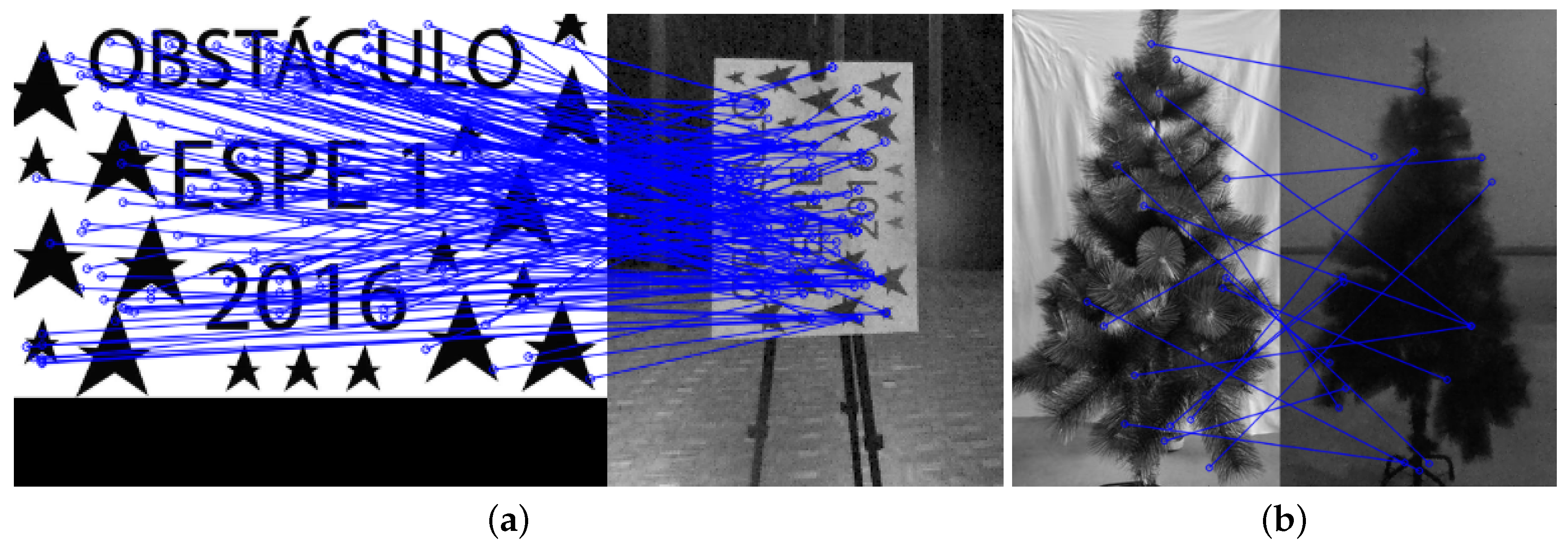
3.1.3. Feature Point Matching

The first challenge for the avoidance system is to detect the obstacle. For this reason, it is necessary to find the correspondence between the image from the database and the image captured by the onboard camera from the MAV. This matching process is based on the vectorial distance between descriptors of each feature point in both images.

The sign of the Laplacian is used for fast feature point indexing it because distinguishes a bright region on a dark background. We only compare the feature points with the same type of contrast, achieving a lower computational cost without reducing the descriptor performance. Additionally, we use Random Sample Consensus (RANSAC) [41,42] to discard the set of the pairs of points out of the model, as shown in Figure 3.

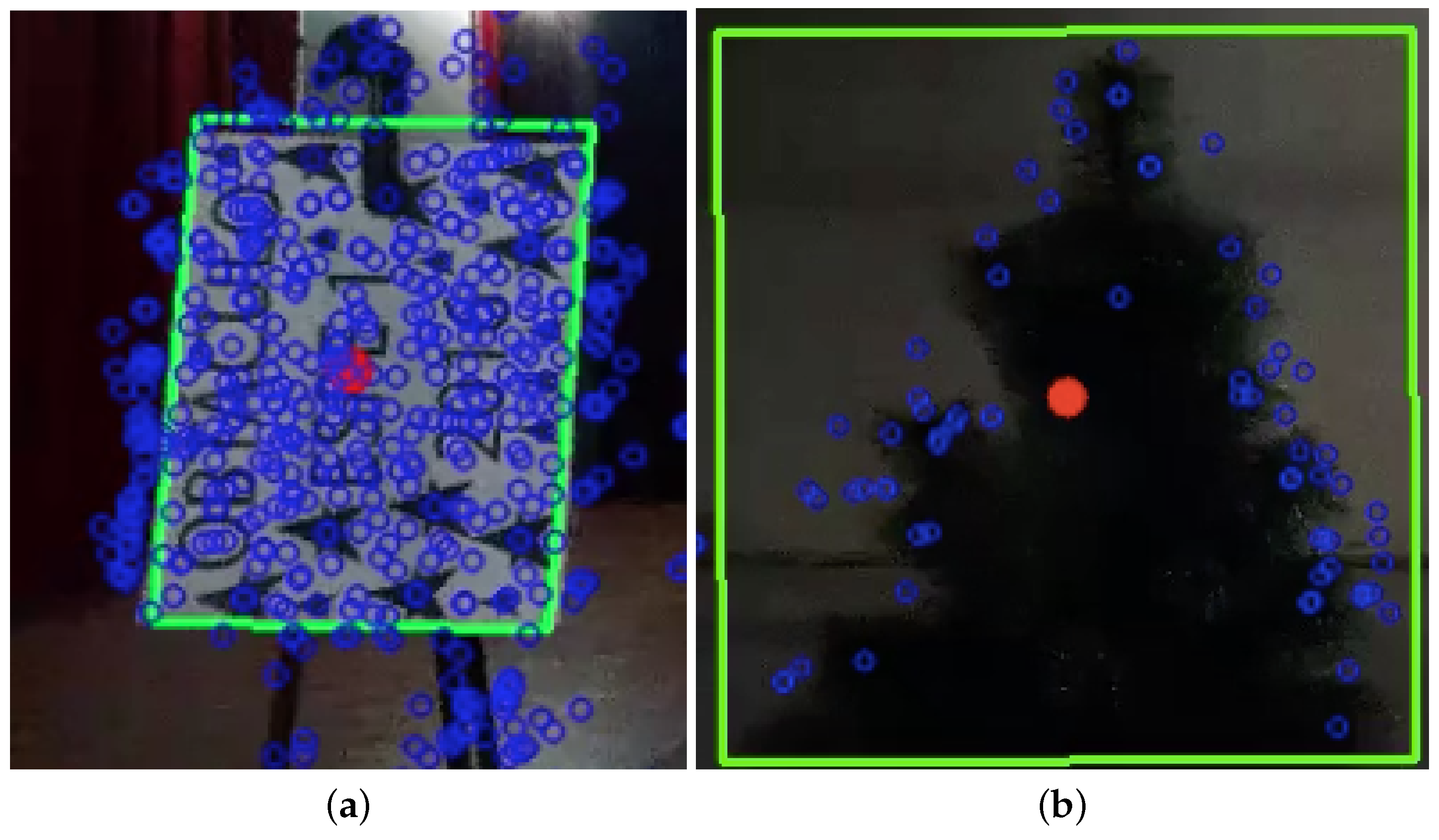
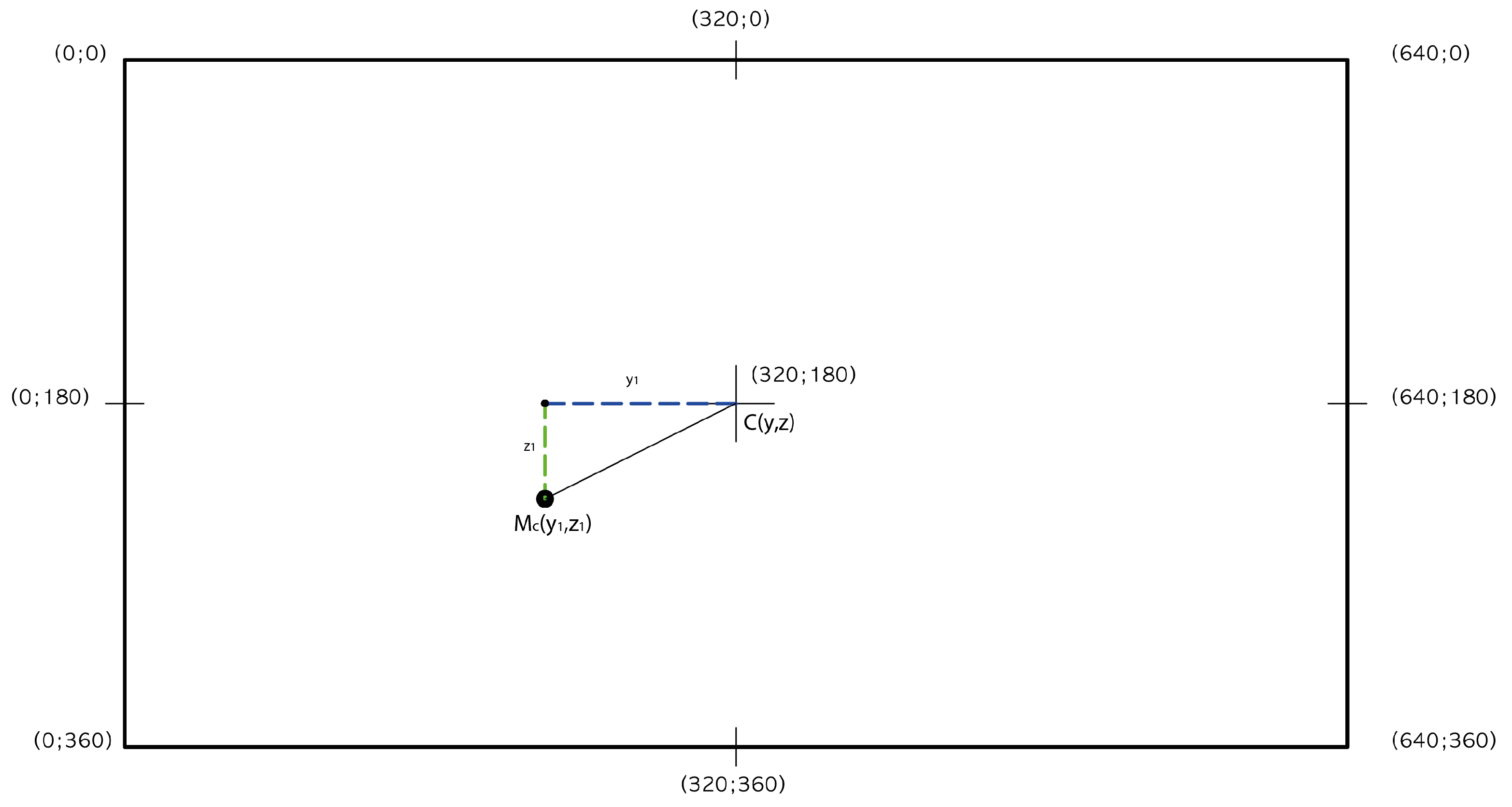
3.2. Obstacle Area and Mass Center

Previous works [43,44,45,46] have made experimental tests with handheld devices and onboard cameras, and the results showed undesired movements and parasitic vibrations that are significant on the plane perpendicular to the roll axis. The distortion can be modeled by a projective transformation; in our case, we use the affine model, which is a particular case of this [47]. The affine transformation is widely used for motion compensation in MAVs. This transformation is mathematically expressed as:

$$\left[\begin{array}{c}{x}_t\\ y_t\\ 1\end{array}\right]=\mathbf{R}\times \left[\begin{array}{c}{x}_{t-1}\\ y_{t-1}\\ 1\end{array}\right]+\mathbf{T}$$

(4)

$$\begin{array}{cc}\hfill \mathbf{R}=\left[\begin{array}{cc}{r}_{00}& r_{01}\\ r_{10}& r_{11}\end{array}\right],& \mathbf{T}=\left[\begin{array}{c}{t}_{00}\\ t_{10}\end{array}\right]\hfill \end{array}$$

(5)

$$\left[\begin{array}{c}{x}_t\\ y_t\\ 1\end{array}\right]=\left[\begin{array}{ccc}{r}_{00}& r_{01}& n_{00}\\ r_{10}& r_{11}& n_{10}\\ 1& 1& 1\end{array}\right]\times \left[\begin{array}{c}{x}_{t-1}\\ y_{t-1}\\ 1\end{array}\right]$$

(6)

where R is the rotation matrix for roll (Figure 4), T is the translation in x and y, $x_{t-1}$ and $y_{t-1}$ are the coordinates of each pixel on the last image and $x_t$ and $y_t$ are the coordinates of each pixel on the current image.

We generate a bounding box for each obstacle defined by a, b, c and d, as shown in Figure 5.

These points are warped on the image captured with the onboard camera, and we use the affine transformation to compensate this warping:

$$I_t=\mathbf{H}\times I_{t-1}$$

(7)

where $I_t$ represents the current image function, $I_{t-1}$ is the last image function and H is the affine transformation matrix. Finally, we calculate the area defined by the compensated vertex a to d. Due to the rectangle being a regular figure, we estimate the mass center $M_c$ by the average value of the x and y coordinates of each vertex, as shown in Figure 6.

4. Obstacle Avoidance

The obstacle avoidance process of our proposal is separated into three parts:

• System identification,
• Controller design,
• Obstacle avoidance algorithm.

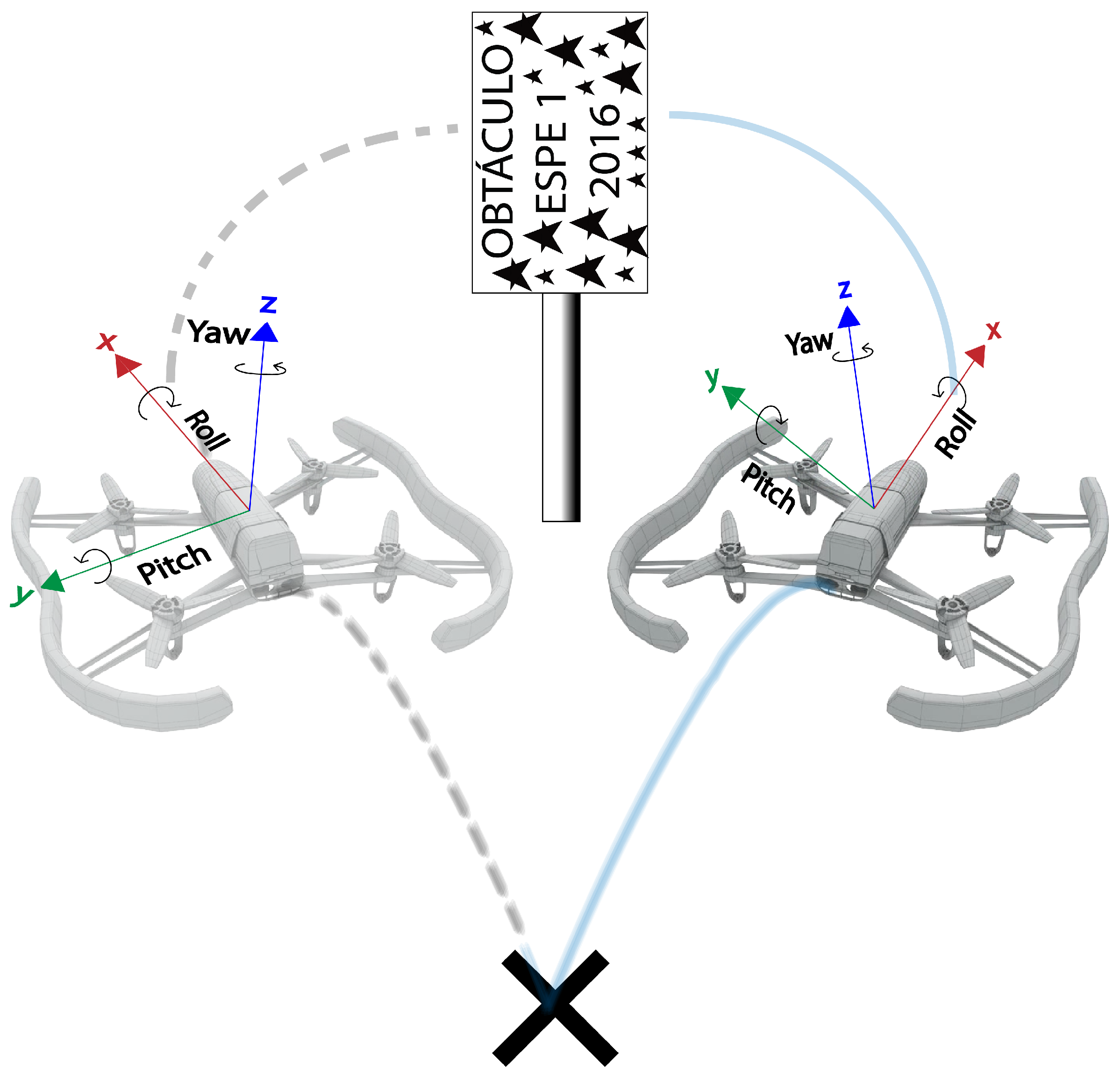
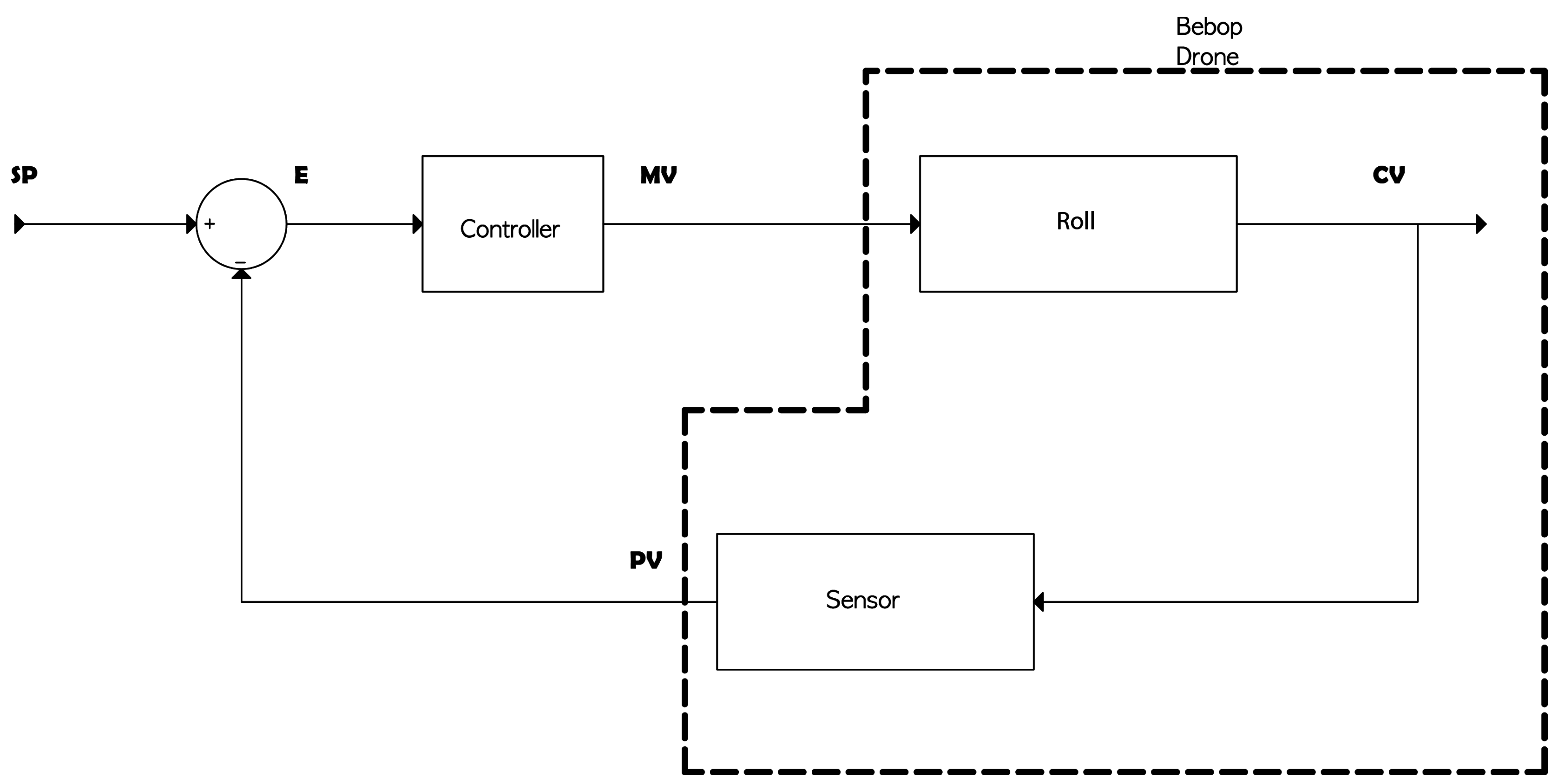
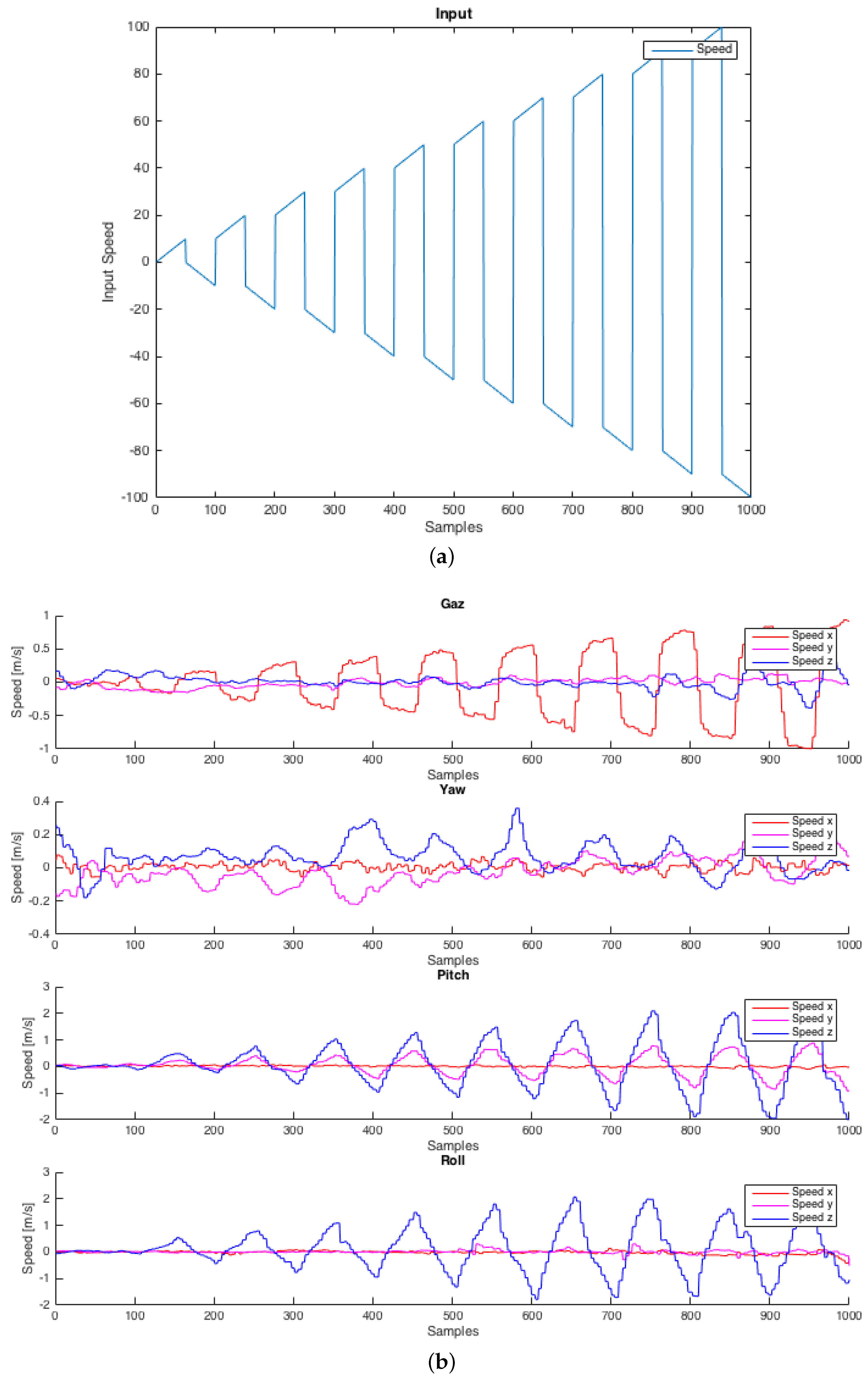
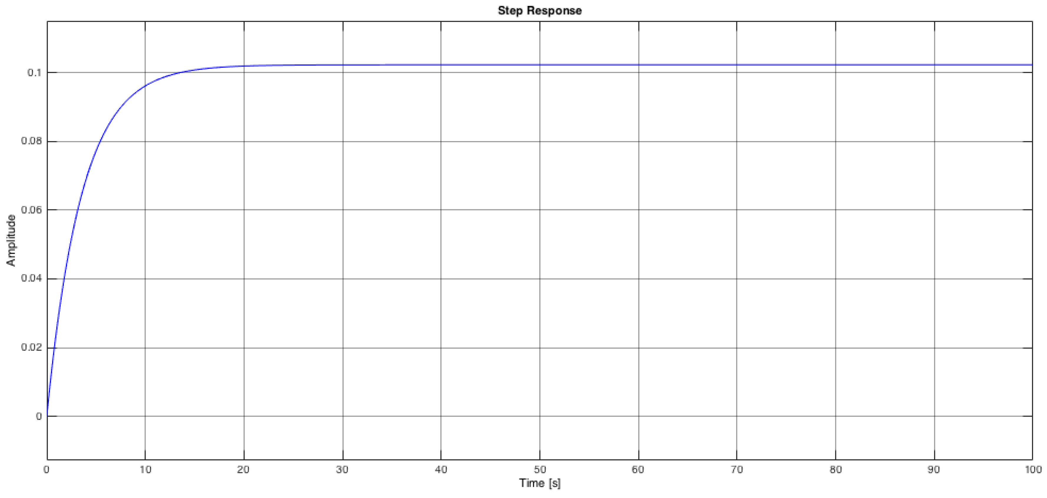
4.1. System Identification

The platform used in the experimentation is the Bebop Drone 1, a low-cost MAV built by the company Parrot. This vehicle was selected for several reasons: low cost, energy conservation, stable flying and vehicle size. The Bebop Drone can be controlled by smartphones or tablets with the operation systems iOS or Android. Furthermore, Parrot has opened the SDK (Software Develop Kit) for operating systems like Linux and Windows, so it can be controlled with a laptop/desktop computer. The control system of the Bebop Drone manipulates four different control actions: pitch, roll, yaw and altitude. Inertial Measurement Unit (IMU) and control action data were collected from the Bebop Drone for model identification. In our model, we use control actions as input (Figure 7a) and velocities as outputs (Figure 7b). We proposed two motions in the planes x and y for the avoidance system; in the x-axis, the motion is uniform, i.e., the linear speed x is constant. The motion in the y-axis depends on the obstacle location, so the control law will be applied to this axis.

Based on the low-level control system of Bebop, the motion in the y-axis can be controlled by the roll [48,49]. It is necessary to estimate the mathematical model that relates roll control with the linear speed in the y-axis; the transfer function of the mathematical model is shown in Equation (8). This model is simulated and presented in Figure 8 in order to observe the step response. It is important to mention that the system is stable and has a slow setting time.

$$G\left(s\right)=\frac{K}{Ts+1}$$

(8)

4.2. Controller Design

One consideration of the controller is that after detecting the obstacle, the vehicle should recover the path. Additionally, we must define if the obstacle is on the flight trajectory, the position error and the target area-based distance between the obstacle and the MAV. As shown on Figure 9.

4.2.1. Position Error

The visual field of the drone depends on the resolution of the camera. For the bebop drone, we capture 640 × 480 pixels for each image, where the obstacles are defined by the mass center as $M_c(y,z)$ in the visual field image (Figure 10). The position error $e\left(t\right)$ is the difference between the obstacle mass center and the center $C(y,z)$ of the image (visual field).

$$e\left(t\right)=C(y,z)-M_c(y,z)$$

(9)

The position error is the mathematical expression of the distance between the MAV and the obstacles. If e(t) < 0, the obstacle is located on the right side of the drone; otherwise, the obstacle is on the left side. The maximum and minimum values of the error are −320 and 320 for the y-axis.

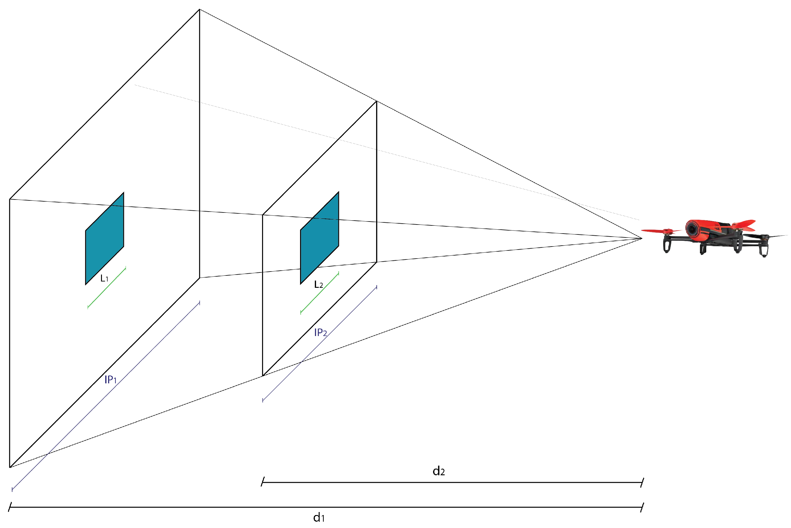
4.2.2. Obstacle Area

The obtained area is proportional to the distance between the onboard camera and the obstacle. In Figure 11, the relation between the image plane and the obstacle length is graphically explained:

$$\begin{array}{c}\hfill \frac{L_1}{I{P}_1}=\frac{L_{p1}}{I{P}_{p1}}\end{array},\begin{array}{c}\hfill \frac{L_2}{I{P}_2}=\frac{L_{p2}}{I{P}_{p2}}\end{array}$$

(10)

where $L_1$ and $L_2$ are the obstacle lengths, $L_{p1}$ and $L_{p2}$ are the obstacle lengths in pixels, $I{P}_1$ and $I{P}_2$ are the image plane lengths and the image plane lengths in pixels are represented by $I{P}_{p1}$ and $I{P}_{p2}$. $I{P}_{p1}=I{P}_{p2}$, because they do not depend on the position of the image plane:

$$\frac{L_{p1}}{L_{p2}}=\frac{L_1\times I_{p2}}{L_2\times I_{p1}},L_1=L_2$$

(11)

$$\frac{L_{p1}}{L_{p2}}=\frac{I_{p2}}{I_{p1}}$$

(12)

If $L_{p2}>L_{p1}$, the image plane $I_{p2}$ increases; otherwise, $I_{p2}$ decreases; this represents varying of the obstacle dimensions from different perspectives. Furthermore, the image plane has a relation to the distance between the MAV and obstacle, as shown:

$$\frac{I_{p1}}{I_{p2}}=\frac{d_1}{d_2}$$

(13)

If an obstacle is out of the visual field, it is not detected because it is far from the UAV and does not interfere with the flight path.

4.2.3. Proportional Controller

The objective of most control systems is reducing to zero the error between the output and set point. However, for the avoidance system (Figure 12), the controller increases the difference between the obstacle’s mass center and the visual field center. If the position error is low, i.e., the obstacle is close to the path center, the control system must send a higher speed signal to the motor controllers in order to keep distance with respect to obstacles. On the other hand, when the position error is higher, the obstacle is far from the path center, reducing the collision probability. The control law depends on the location of the obstacle; it is positive when the error is $e\left(t\right)<0$ and negative when $e\left(t\right)>0$ (Figure 13). This means that the controller output $u\left(t\right)$ is inversely proportional to the error $e\left(t\right)$.

We are using a proportional controller, which automatically compensates the environmental disturbance and provides a smooth, continuous and linear control function, as mentioned by Hughes in [50]. Our experimental results show that our approach has a higher performance than the bang-bang controller. We obtained a control law with a proportional gain $Kp$ and a bias P, defined as:

$$u\left(t\right)=Kp\times e\left(t\right)+P$$

(14)

4.2.4. Translation Compensation

In addition to avoidance, the MAV needs to return to the path; in our proposal, we compensate the deviation of the MAV when avoiding the obstacle (Figure 14). To do this, we use the average speed $r\left(t\right)$ of the control signal $u\left(t\right)$ (Equation (15)).

$$ur\left(t\right)=\left(\frac{{\sum }_{i=1}^{n}u\left(i\right)}{n}\right)\times (-1)$$

(15)

Furthermore, for that, the MAV gets to the goal and returns on the path; we used a target tracking. When the MAV detects the image that indicates the end of flight, at first, it does the tracking with a control law and then lands. The target tracking works with the position error $e\left(t\right)$ and a proportional controller. However, without a position estimation method, the vehicle could be susceptible to position drift caused by external disturbances or slight variations in orientation. The position estimation is proposed for future works; for the moment, we perform the experiments in a controller environment with minimal external disturbances.

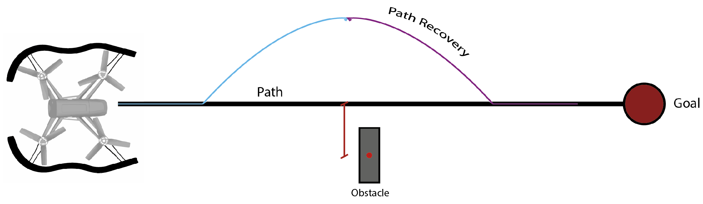
4.3. Obstacle Avoidance and Path Recovery Algorithm

Our proposal of obstacle avoidance is described in the Algorithm 1. Our algorithm starts when the obstacle area is greater than the limit area; this means that the vehicle is closer to the obstacle than the distance allowed. The limit area value is experimentally obtained defining the dimensions of obstacles in pixels at a specific distance. The output $u\left(t\right)$ of the control law moves the vehicle away from the center of the obstacle avoiding it. If the error is greater than zero, the MAV moves to the left side; otherwise, the vehicle moves to the right side.

Algorithm 2 shows the path recovery that uses the average speed $ur\left(t\right)$ obtained from the control signal $u\left(t\right)$ to compensate the deviation of the MAV in the avoidance.

Algorithm 1 Obstacle avoidance algorithm.
1: if $area>are{a}_{exp}$ then   2:       $u\left(t\right)=kp\times e\left(t\right)+P$   3:       if $e\left(t\right)<0$ then   4:           $u\left(t\right)=u\left(t\right)\times (-sign(e\left(t\right)\left)\right)$   5:       end if   6:       if $e\left(t\right)>0$ then   7:           $u\left(t\right)=u\left(t\right)\times \left(sign\right(e\left(t\right)\left)\right)$   8:       end if   9: end if 10: if $area\ge 0\mathbf{and}area<are{a}_{exp}$ then 11:       $u\left(t\right)=0$ 12: end if 13: $spee{d}_{acc}=spee{d}_{acc}+u\left(t\right)$ 14: $n=n+1$
Parameters
$area:$	obstacle area
$are{a}_{exp}:$	limit area
$e\left(t\right):$	position error, between the path center and mass center of obstacle
$u\left(t\right):$	speed that will be sent to MAV
$spee{d}_{acc}:$	speed accumulated during the period of avoidance
$n:$	numbers of speed data saved

Algorithm 2 Path recovery algorithm.
1: $ur\left(t\right)=spee{d}_{acc}/n$ 2: $u\left(t\right)=ur\left(t\right)\times (-1)$ 3: $time.sleep\left(\right)$ 4: $u\left(t\right)=kp\times e\left(t\right)+P$ 5: if $area>are{a}_{exp}$ then 6:       $land\left(\right)$ 7: end if
Parameters
$ur\left(t\right):$	average speed
$time.sleep\left(\right):$	wait time
$Land\left(\right):$	landing of the MAV

In Figure 15, we present our full obstacle avoidance algorithm.

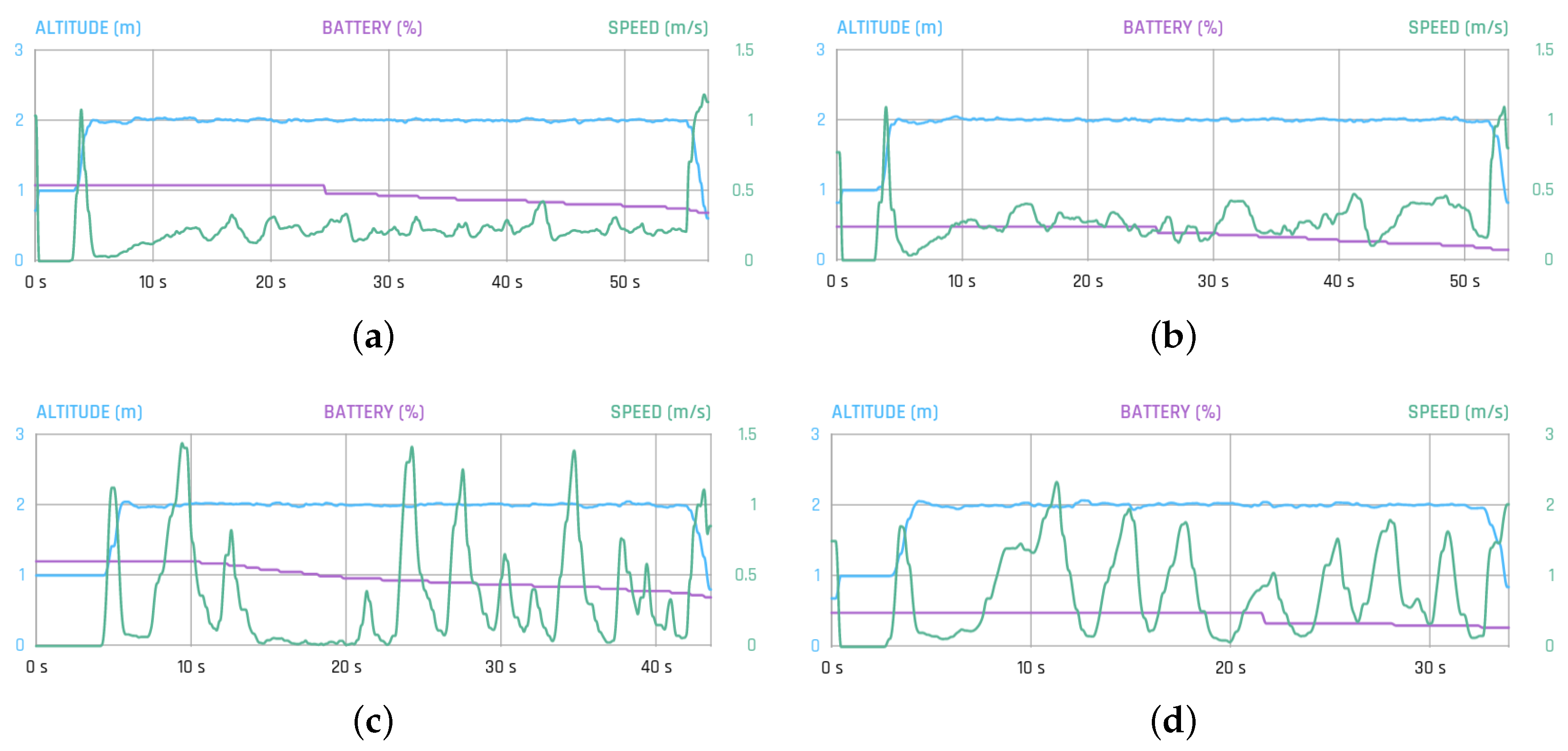
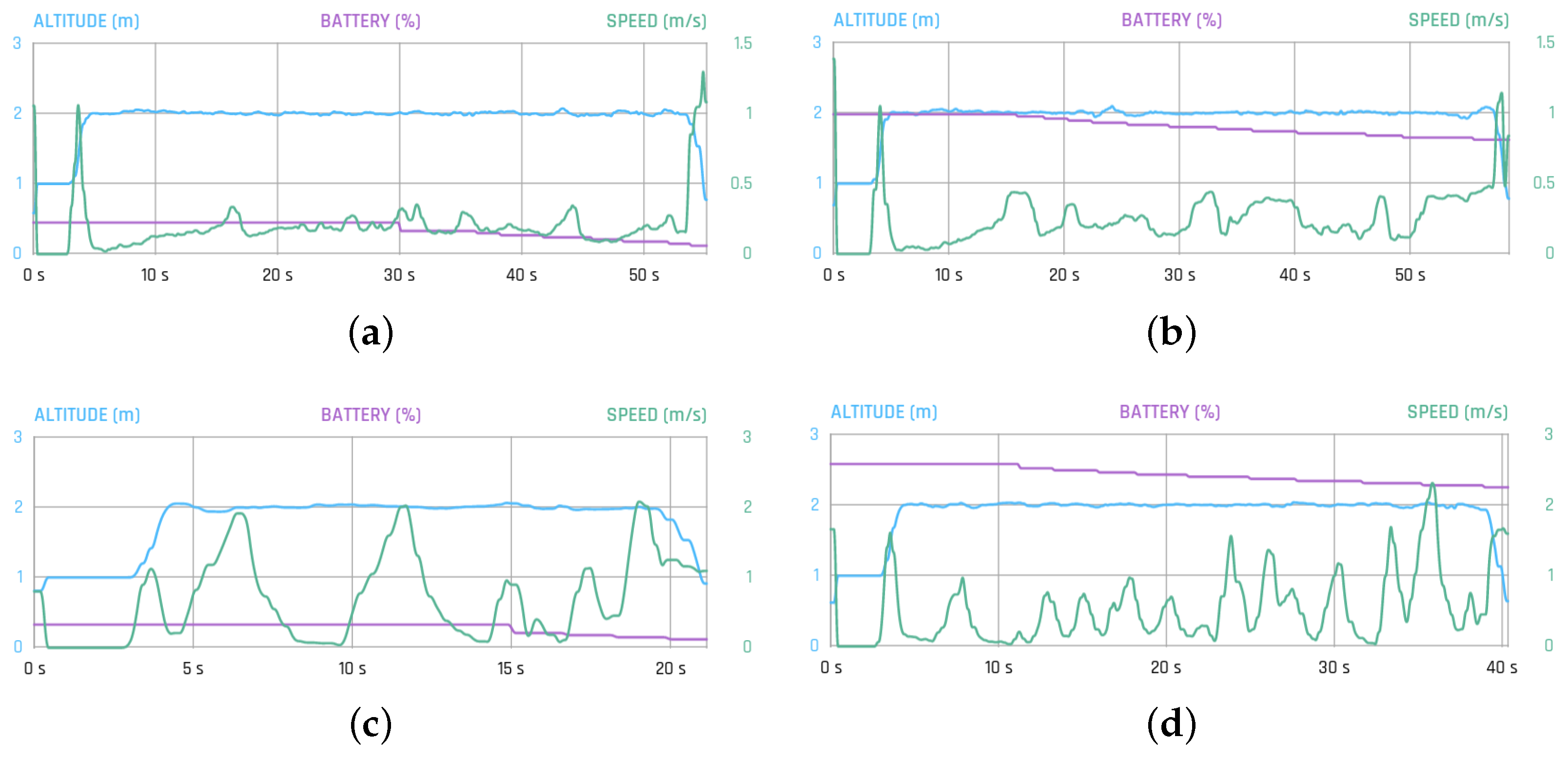
5. Experiments and Results

The Bebop Drone is connected by WiFi to a laptop with the following characteristics: processor Intel Core i7-2670QM Quad-Core 2.2 GHz and 8.00 GB RAM running Linux. The laptop is destined to processes the obstacle detection and avoidance algorithms. We have used the Katarina open-source library developed by Dlouhý [51] for communication of the laptop with the MAV and obtain images in real time from the monocular onboard camera of the MAV.

We performed an experimental comparison between our autonomous algorithm, the algorithm proposed by [30] and the teleoperation of two persons with different experience levels, using the same MAV. Additionally, we performed an experiment that compares our algorithm in different scenarios.

The metrics of evaluation are:

• Time: This shows the necessary time to complete the path.
• Maximum speed: This is an indicator proportional to the maximum distance to the rectilinear path.
• Minimum speed: This is an indicator proportional to the minimum distance to the rectilinear path.
• Average speed: This is an indicator proportional to the average distance to the rectilinear path.
• Distance: This shows the traveled distance of the flight.
• Battery: This shows the ratio of the battery used on the flight.
• Successful flights: This shows the number of flights that completed the path without the MAV touching or hitting the obstacles.
• Unsuccessful flights: This shows the number of flights that did not complete the path, due to the MAV touching or hitting the obstacles.

The experiments were performed in different controlled scenarios as shown on the Figure 16, Figure 17, Figure 18, Figure 19, , Figure 20 and Figure 21:

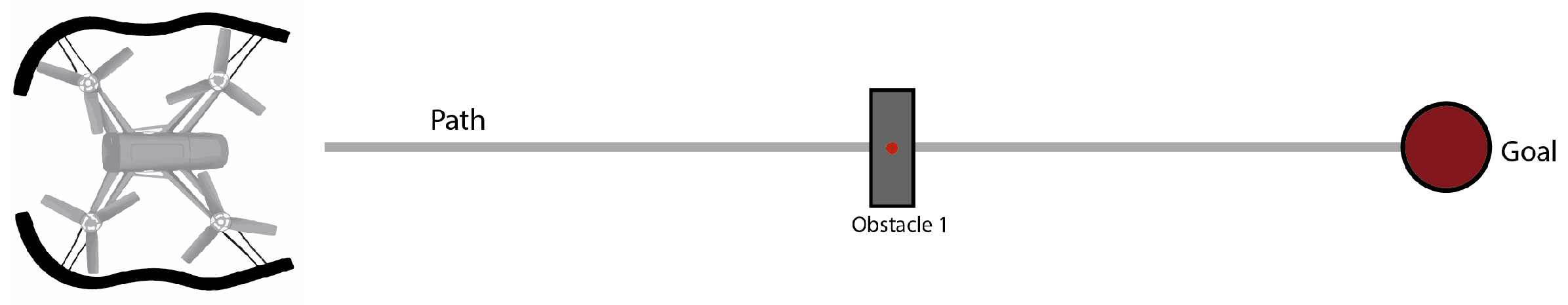
• One fixed obstacle.
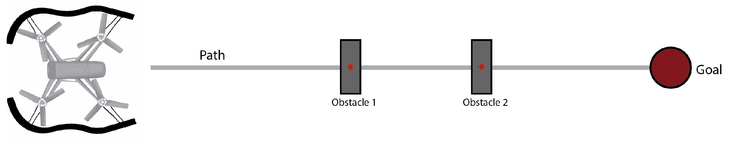
• Two fixed obstacles.
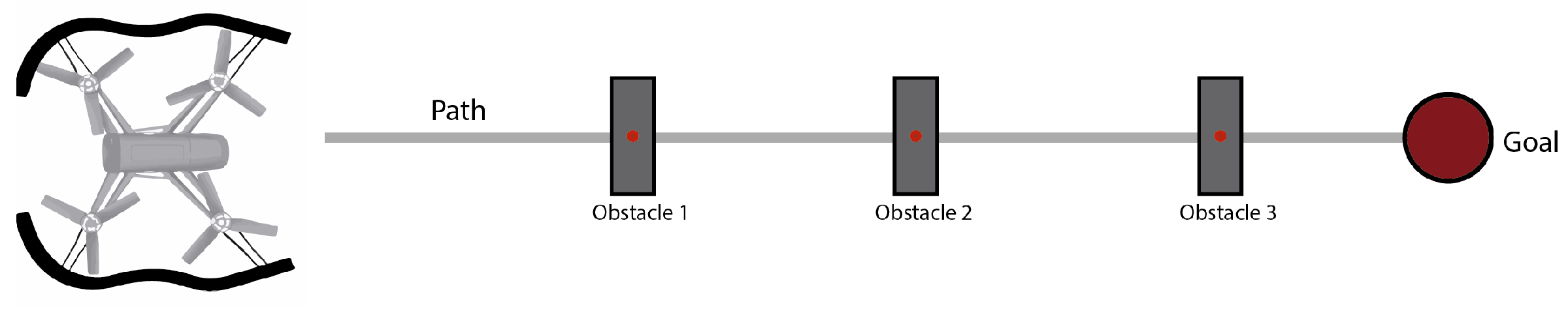
• Three fixed obstacles.
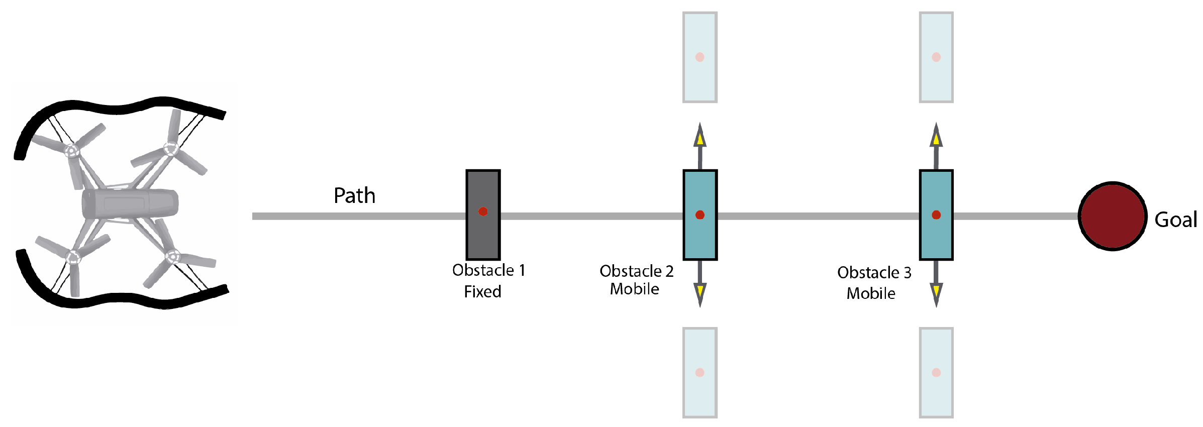
• One fixed obstacle and two mobile obstacles.
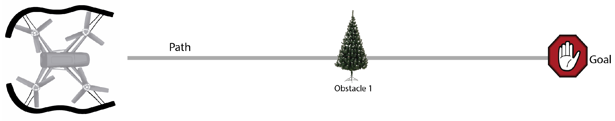
• One tree.
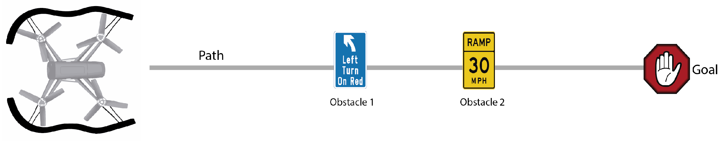
• Two traffic signs.

Figure 22, Figure 23, Figure 24 and Figure 25 show the results of one flight in different scenarios;

Table 1. One fixed obstacle.

Control	Maximum Speed (m/s)	Minimum Speed (m/s)	Average Speed (m/s)	Distance (m)	Time (s)	Battery (%)
Autonomous algorithm	0.865	0.116	0.256	4.957	18.869	5.389
Bang-Bang	0.918	0.108	0.290	5.262	18.207	5.422
Teleoperator with experience	2.625	0.108	1.073	8.716	9.817	5.750
Teleoperator without experience	2.313	0.141	0.809	9.490	11.997	6.692

,

Table 2. Two fixed obstacles.

Control	Maximum Speed (m/s)	Minimum Speed (m/s)	Average Speed (m/s)	Distance (m)	Time (s)	Battery (%)
Autonomous algorithm	0.780	0.113	0.252	8.582	33.382	8.811
Bang-Bang	0.832	0.109	0.320	10.227	33.075	9.419
Teleoperator with experience	1.862	0.112	0.597	12.879	23.104	7.291
Teleoperator without experience	1.585	0.108	0.543	12.813	26.660	9.664

,

Table 3. Three fixed obstacles.

Control	Maximum Speed (m/s)	Minimum Speed (m/s)	Average Speed (m/s)	Distance (m)	Time (s)	Battery (%)
Autonomous algorithm	0.940	0.104	0.253	11.914	46.143	11.536
Bang-Bang	0.952	0.108	0.276	13.120	46.633	15.357
Teleoperator with experience	2.646	0.104	0.626	21.056	48.418	6.321
Teleoperator without experience	2.791	0.106	0.987	32.123	48.887	7.361

and

Table 4. One fixed obstacle and two mobile obstacles.

Control	Maximum Speed (m/s)	Minimum Speed (m/s)	Average Speed (m/s)	Distance (m)	Time (s)	Battery (%)
Autonomous algorithm	0.760	0.104	0.235	11.759	48.271	13.888
Bang-Bang	0.942	0.108	0.304	16.997	51.800	13.184
Teleoperator with experience	2.189	0.118	0.915	15.859	20.490	11.390
Teleoperator without experience	2.910	0.103	0.767	22.040	34.038	12.419

present the average values of the experimental successfully flights; and

Table 5. Results of flights with different controls.

Control	Total Number of Flights	Successful Flights	Unsuccessful Flights	Successful Flights Ratio (%)
Autonomous algorithm	20	16	4	80
Bang-Bang	20	12	8	60
Teleoperator with experience	20	13	7	65
Teleoperator without experience	20	11	9	55

a summary of them. For the last experimental test with one tree and two traffic signs, the results are shown in Figure 26;

Table 6. Tree and traffic sign obstacles.

Obstacle-Type	Maximum Speed (m/s)	Minimum Speed (m/s)	Average Speed (m/s)	Distance (m)	Time (s)	Battery (%)
Pre-designed obstacle	0.865	0.116	0.256	4.957	18.869	5.389
Tree	0.303	0.028	0.124	3.025	24.121	3.432
Traffic signs	0.634	0.052	0.241	5.928	27.620	5.625

presents the average values of successful flights; and

Table 7. Results of flights with tree and traffic sign obstacles.

Obstacle-Type	Total Number of Flights	Successful Flights	Unsuccessful Flights	Successful Flights Ratio (%)
Pre-designed obstacle	10	8	2	80
Tree	10	4	6	40
Traffic signs	10	8	2	80

shows the number of flights that completed the path. The normalized values were obtained from the official Android App of Parrot. The numbers in bold on the tables mean the best result in the experiment.

Experimental results with the fixed obstacle showed that the autonomous system has a lower ratio of battery usage and traveled distance, due to the system not having high variations of speed. The teleoperators used the least time to complete the path, for the ease of avoiding one obstacle, but if we compared with the bang-bang system, the time is similar.

The results of two fixed obstacle showed that our algorithm has a lower traveled distance because it can keep a stable speed better than the others. The time to complete the path and battery usage are less for the teleoperator with experience. In this case, our algorithm has a similar time with respect to completing the path with the bang-bang controller.

The high performance of our algorithm is evidenced on experimentation with three fixed obstacles because unlike the human teleoperators, our autonomous system has no fatigue issues. The average speed, traveled distance and the time to complete the path are lower than others. The battery usage is less for the teleoperator with experience due to using more speed in several cases, but increases the probability of collision.

For one fixed and two mobiles obstacles, the challenge is greater because at any time, an obstacle can be present in the environment and produce a collision. In this case, our algorithm presents a good response, as shown in Table 4; the traveled distance and the average speed are lower than others. The time to complete the path is lower for teleoperators, but in Table 5, we can see that they have more unsuccessful flights than our proposal due to using higher speeds, increasing the probability of collisions.

The results of the experiments performed to know how our autonomous system responds in different scenarios are presented in Table 6 and Table 7. They demonstrate that our proposal has a good performance. When it works with traffic signs and a pre-designed obstacle, the number of successful flights is high because the average values do not have a greater variety; and when the tree is an obstacle, the results showed that our algorithm can avoid this, but the number of successful flights is low. To improve this, we will address this problem in future works.

Based on the experimental results, our proposal has a better performance than the bang-bang controller and the teleoperators because the traveled distance and the time are lower, and additionally, the stable speed allows successful flights. In spite of the use of the battery and the average time required to complete the path is lower for teleoperators, the number of unsuccessful flights’ ratio is higher. When the number of obstacles is higher, the performance of human teleoperators decreases, as a consequence of fatigue; on the other hand, our proposal keeps this performance. Unlike the bang-bang controller, our proposal includes a path recovery system in order to return to the original trajectory. The importance of the path recovery system is evident when increasing the number of obstacles; for example: for two or more obstacles, the bang-bang controller avoids the first obstacle and loses the path for the next obstacles, ending in another location. Our approach finishes in the correct goal.

Video results are provided in [52].

6. Conclusions and Future Works

In this paper, we experimentally tested the optimal and robust performance of our system, including obstacle detection and avoidance.

Flexibility and energy efficiency are important features for autonomous navigation of UAVs. In our approach, flexibility is given by the effectiveness responding to the unspecified number of obstacles in unknown positions. SURF obtains matching between the image from the database and captured frame without incrementing the computational cost.

Our proportional controller for obstacle avoidance between the start and goal point is optimal, faster and has higher performance than a bang-bang controller, as well as human controllers with and without experience.

For future works, we will improve the detection algorithm without the use of the database. We will compare use natural key points and a real-time path planning algorithm [53,54].

References

- Barrientos, A.; del Cerro, J.; Gutiérrez, P.; San Martín, R.; Martínez, A.; Rossi, C. Vehículos Aéreos no Tripulados Para Uso Civil. Tecnología y Aplicaciones; Universidad Politécnica de Madrid: Madrid, Spain, 2007. [Google Scholar]
- Kendoul, F. Survey of advances in guidance, navigation, and control of unmanned rotorcraft systems. J. Field Robot. 2012, 29, 315–378. [Google Scholar] [CrossRef]
- Ortega, D.V.; Bueno, J.A.G.C.; Merino, R.V.; Sanz, S.B.; Correas, A.H.; Campo, D.R. Pilotos de Dron (RPAS); Ediciones Paraninfo S.A.: Madrid, Spain, 2005. [Google Scholar]
- Scherer, S.; Singh, S.; Chamberlain, L.; Elgersma, M. Flying fast and low among obstacles: Methodology and experiments. Int. J. Robot. Res. 2008, 27, 549–574. [Google Scholar] [CrossRef]
- Sabatini, R.; Gardi, A.; Richardson, M. LIDAR obstacle warning and avoidance system for unmanned aircraft. Int. J. Mech. Aerosp. Ind. Mechatron. Eng. 2014, 8, 718–729. [Google Scholar]
- Sabatini, R.; Gardi, A.; Ramasamy, S.; Richardson, M.A. A laser obstacle warning and avoidance system for manned and unmanned aircraft. In Proceedings of the MetroAeroSpace 2014: IEEE Workshop on Metrology for Aerospace, Benevento, Italy, 29–30 May 2014; pp. 616–621.
- Kerl, C. Odometry from RGB-D Cameras for Autonomous Quadrocopters. Ph.D. Thesis, Technischen Universitat Munchen (LUM), Munchen, Germany, 2012. [Google Scholar]
- Bachrach, A.; Prentice, S.; He, R.; Henry, P.; Huang, A.S.; Krainin, M.; Maturana, D.; Fox, D.; Roy, N. Estimation, planning, and mapping for autonomous flight using an RGB-D camera in GPS-denied environments. Int. J. Robot. Res. 2012, 31, 1320–1343. [Google Scholar] [CrossRef]
- Beyeler, A.; Zufferey, J.C.; Floreano, D. 3D vision-based navigation for indoor microflyers. In Proceedings of the 2007 IEEE International Conference on Robotics and Automation, Roma, Italy, 10–14 April 2007; pp. 1336–1341.
- Oh, P.Y.; Green, W.E.; Barrows, G. Neural nets and optic flow for autonomous micro-air-vehicle navigation. In Proceedings of the ASME 2004 International Mechanical Engineering Congress and Exposition, Anaheim, CA, USA, 13–19 November 2004; American Society of Mechanical Engineers: New York, NY, USA, 2004; pp. 1279–1285. [Google Scholar]
- Zufferey, J.C.; Floreano, D. Fly-inspired visual steering of an ultralight indoor aircraft. IEEE Trans. Robot. 2006, 22, 137–146. [Google Scholar] [CrossRef]
- Muratet, L.; Doncieux, S.; Meyer, J.A. A biomimetic reactive navigation system using the optical flow for a rotary-wing UAV in urban environment. In Proceedings of the International Symposium on Robotics ISR, Paris, France, 23–26 March 2004.
- Merrell, P.C.; Lee, D.J.; Beard, R.W. Obstacle Avoidance for Unmanned Air Vehicles Using Optical Flow Probability Distributions; International Society for Optics and Photonics: Bellingham, WA, USA, 2004; pp. 13–22. [Google Scholar]
- Green, W.E.; Oh, P.Y. Optic-flow-based collision avoidance. IEEE Robot. Autom. Mag. 2008, 15, 96–103. [Google Scholar] [CrossRef]
- Sabe, K.; Fukuchi, M.; Gutmann, J.S.; Ohashi, T.; Kawamoto, K.; Yoshigahara, T. Obstacle avoidance and path planning for humanoid robots using stereo vision. In Proceedings of the 2004 IEEE International Conference on Robotics and Automation (ICRA’04), New Orleans, LA, USA, 26 April–1 May 2004; Volume 1, pp. 592–597.
- Na, I.; Han, S.H.; Jeong, H. Stereo-based road obstacle detection and tracking. In Proceedings of the 2011 13th International Conference on Advanced CommunicationTechnology (ICACT), Gangwon-Do, Korea, 13–16 February 2011.
- Bills, C.; Chen, J.; Saxena, A. Autonomous MAV flight in indoor environments using single image perspective cues. In Proceedings of the 2011 IEEE International Conference on Robotics and Automation (ICRA), Shanghai, China, 9–13 May 2011; pp. 5776–5783.
- Çelik, K.; Somani, A.K. Monocular vision SLAM for indoor aerial vehicles. J. Electr. Comput. Eng. 2013, 2013, 1566–1573. [Google Scholar] [CrossRef]
- De Croon, G.; De Weerdt, E.; De Wagter, C.; Remes, B.; Ruijsink, R. The appearance variation cue for obstacle avoidance. IEEE Trans. Robot. 2012, 28, 529–534. [Google Scholar] [CrossRef]
- Lin, Y.; Saripalli, S. Moving obstacle avoidance for unmanned aerial vehicles. In Proceedings of the 69th American Helicopter Society International Annual Forum 2013, Phoenix, AZ, USA, 21–23 May 2013.
- Mejias, L.; Bernal, I.F.M.; Campoy, P. Vision Based Control for Micro Aerial Vehicles: Application to Sense and Avoid. In Recent Advances in Robotics and Automation; Springer: Berlin/Heidelberg, Germany, 2013; pp. 127–141. [Google Scholar]
- Lin, Y.; Saripalli, S. Path planning using 3D dubins curve for unmanned aerial vehicles. In Proceedings of the 2014 IEEE International Conference on Unmanned Aircraft Systems (ICUAS), Orlando, FL, USA, 27–30 May 2014; pp. 296–304.
- Pettersson, P.O.; Doherty, P. Probabilistic roadmap based path planning for an autonomous unmanned helicopter. J. Intell. Fuzzy Syst. 2006, 17, 395–405. [Google Scholar]
- Hrabar, S. 3D path planning and stereo-based obstacle avoidance for rotorcraft UAVs. In Proceedings of the 2008 IEEE/RSJ International Conference on Intelligent Robots and Systems, Nice, France, 22–26 September 2008; pp. 807–814.
- Chavez, A.; Gustafson, D. Vision-based obstacle avoidance using SIFT features. In Proceedings of the International Symposium on Visual Computing, Las Vegas, NV, USA, 30 November–2 December 2009; Springer: Berlin/Heidelberg, Germany, 2009; pp. 550–557. [Google Scholar]
- Kim, D.; Dahyot, R. Face components detection using SURF descriptors and SVMs. In Proceedings of the 2008 International Machine Vision and Image Processing Conference (IMVIP’08), Dublin, Ireland, 3–5 September 2008; pp. 51–56.
- Chu, D.M.; Smeulders, A.W. Color invariant surf in discriminative object tracking. In Proceedings of the 11th European Conference on Computer Vision, Heraklion, Greece, 10–11 September 2010; Springer: Berlin/Heidelberg, Germany, 2010; pp. 62–75. [Google Scholar]
- He, W.; Yamashita, T.; Lu, H.; Lao, S. Surf tracking. In Proceedings of the 2009 IEEE 12th International Conference on Computer Vision, Kyoto, Japan, 29 September–2 October 2009; pp. 1586–1592.
- Krajník, T.; Nitsche, M.; Pedre, S.; Přeučil, L.; Mejail, M.E. A simple visual navigation system for an UAV. In Proceedings of the 2012 IEEE 9th International Multi-Conference on Systems, Signals and Devices (SSD), Chemnitz, Germany, 20–23 March 2012; pp. 1–6.
- Mori, T.; Scherer, S. First results in detecting and avoiding frontal obstacles from a monocular camera for micro unmanned aerial vehicles. In Proceedings of the 2013 IEEE International Conference on Robotics and Automation (ICRA), Karlsruhe, Germany, 6–10 May 2013; pp. 1750–1757.
- Canny, J. A computational approach to edge detection. IEEE Trans. Pattern Anal. Mach. Intell. 1986, PAMI-8, 679–698. [Google Scholar] [CrossRef]
- Harris, C.; Stephens, M. A combined corner and edge detector. In Proceedings of the 4th Alvey Vision Conference, Manchester, UK, 31 August–2 September 1988; Volume 15, p. 50.
- Miksik, O.; Mikolajczyk, K. Evaluation of local detectors and descriptors for fast feature matching. In Proceedings of the 2012 IEEE 21st International Conference on Pattern Recognition (ICPR), Tsukuba, Japan, 11–15 November 2012; pp. 2681–2684.
- Rublee, E.; Rabaud, V.; Konolige, K.; Bradski, G. ORB: An efficient alternative to SIFT or SURF. In Proceedings of the 2011 IEEE International Conference on Computer Vision, Barcelona, Spain, 6–13 November 2011; pp. 2564–2571.
- Alahi, A.; Ortiz, R.; Vandergheynst, P. Freak: Fast retina keypoint. In Proceedings of the 2012 IEEE Conference on Computer Vision and Pattern Recognition (CVPR), Rhode Island, Providence, USA, 16–21 June 2012; pp. 510–517.
- Leutenegger, S.; Chli, M.; Siegwart, R.Y. BRISK: Binary robust invariant scalable keypoints. In Proceedings of the 2011 IEEE International Conference on Computer Vision, Barcelona, Spain, 6–13 November 2011; pp. 2548–2555.
- Lowe, D.G. Object recognition from local scale-invariant features. In Proceedings of the Seventh IEEE International Conference on Computer vision, Kerkyra, Greece, 20–25 September 1999; Volume 2, pp. 1150–1157.
- Bay, H.; Ess, A.; Tuytelaars, T.; van Gool, L. Speeded-up robust features (SURF). Comput. Vis. Image Underst. 2008, 110, 346–359. [Google Scholar] [CrossRef]
- Juan, L.; Gwun, O. A comparison of sift, pca-sift and surf. Int. J. Image Process. (IJIP) 2009, 3, 143–152. [Google Scholar]
- Huang, D.S.; Jo, K.H.; Hussain, A. Intelligent Computing Theories and Methodologies. In Proceedings of the 11th International Conference, ICIC 2015, Fuzhou, China, 20–23 August 2015; Springer: Berlin, Germany, 2015; Volume 9226. [Google Scholar]
- Fischler, M.A.; Bolles, R.C. Random sample consensus: A paradigm for model fitting with applications to image analysis and automated cartography. Commun. ACM 1981, 24, 381–395. [Google Scholar] [CrossRef]
- Derpanis, K.G. Overview of the RANSAC algorithm. Image Rochester NY 2010, 4, 2–3. [Google Scholar]
- Aguilar, W.G.; Angulo Bahón, C. Estabilización robusta de vídeo basada en diferencia de nivel de gris. Congr. Cienc. Tecnol. 2013, 8, 1. [Google Scholar]
- Aguilar, W.G.; Angulo, C. Robust video stabilization based on motion intention for low-cost micro aerial vehicles. In Proceedings of the 2014 IEEE 11th International Multi-Conference on Systems, Signals & Devices (SSD), Castelldefels, Spain, 11–14 February 2014; pp. 1–6.
- Aguilar, W.G.; Angulo, C. Real-time video stabilization without phantom movements for micro aerial vehicles. EURASIP J. Image Video Process. 2014, 2014, 1–13. [Google Scholar] [CrossRef]
- Aguilar, W.G.; Angulo, C. Estabilización de vídeo en micro vehículos aéreos y su aplicación en la detección de caras. In Proceedings of the IIX Congreso De Ciencia Y Tecnología ESPE 2014, Sangolquí, Ecuador, 28–30 May 2014; pp. 1–6.
- Vazquez, M.; Chang, C. Real-time video smoothing for small RC helicopters. In Proceedings of the 2009 IEEE International Conference on Systems, Man and Cybernetics (SMC 2009), San Antonio, TX, USA, 11–14 October 2009; pp. 4019–4024.
- Aguilar, W.G.; Angulo, C. Real-Time Model-Based Video Stabilization for Microaerial Vehicles. Neural Proc. Lett. 2016, 43, 459–477. [Google Scholar] [CrossRef]
- Aguilar, W.G.; Angulo, C. Control autónomo de cuadricópteros para seguimiento de trayectorias. In Proceedings of the IX Congreso de Ciencia y Tecnología ESPE, Sangolquí, Ecuador, 28–30 May 2014.
- Hughes, J.M. Real World Instrumentation with Python: Automated Data Acquisition and Control Systems; O’Reilly Media, Inc.: Fort Salvador, CA, USA, 2010. [Google Scholar]
- Dlouhý, M. Katarina. Available online: http://robotika.cz/robots/katarina/en (accessed on 17 October 2016).
- Aguilar, W.G.; Casaliglla, V.P.; Polit, J.L. Obstacle Avoidance for UAVs. Available online: http://www.youtube.com/watch?v=uiN9PgPpFao&feature=youtu.be (accessed on 26 December 2016).
- Aguilar, W.G.; Morales, S.G. 3D environment mapping using the Kinect V2 and path planning based on RRT algorithms. Electronics 2016, 5, 70. [Google Scholar] [CrossRef]
- Cabras, P.; Rosell, J.; Pérez, A.; Aguilar, W.G.; Rosell, A. Haptic-based navigation for the virtual bronchoscopy. IFAC Proc. Vol. 2011, 44, 9638–9643. [Google Scholar] [CrossRef]