Parallel Simulation of Loosely Timed SystemC/TLM Programs: Challenges Raised by an Industrial Case Study ^†

Abstract

Transaction level models of systems-on-chip in SystemC are commonly used in the industry to provide an early simulation environment. The SystemC standard imposes coroutine semantics for the scheduling of simulated processes, to ensure determinism and reproducibility of simulations. However, because of this, sequential implementations have, for a long time, been the only option available, and still now the reference implementation is sequential. With the increasing size and complexity of models, and the multiplication of computation cores on recent machines, the parallelization of SystemC simulations is a major research concern. There have been several proposals for SystemC parallelization, but most of them are limited to cycle-accurate models. In this paper we focus on loosely timed models, which are commonly used in the industry. We present an industrial context and show that, unfortunately, most of the existing approaches for SystemC parallelization can fundamentally not apply in this context. We support this claim with a set of measurements performed on a platform used in production at STMicroelectronics. This paper surveys existing techniques, presents a visualization and profiling tool and identifies unsolved challenges in the parallelization of SystemC models at transaction level.

1. Introduction

The design of SoC (Systems-on-Chip) includes both hardware and software development. The embedded software is dependent on the hardware interfaces, but the hardware design is the most critical step of the flow, because modifying it is very costly. For this reason, a model of the hardware has to be developed. TLM (Transaction Level Modeling) models are highly abstract and enable both the ability to check hardware functionality in terms of data and control exchanges and to debug the embedded software before the detailed microarchitecture is available. Within TLM, multiple coding styles exist, depending on the level of detail needed. If the purpose is to have the earliest and fastest opportunity to run a transaction-accurate simulation of the hardware, for example in the case of a non-critical SoC, then LT (Loosely Timed) style is a relevant choice. Indeed, a TLM/LT simulation runs orders of magnitude faster than an RTL (Register Transfer Level) one.

SystemC is a C++ hardware modeling library which enables TLM, and also an IEEE standard. Since hardware systems are intrinsically parallel systems, the API offered by SystemC supports parallel semantics. The hardware behavior is modeled by SystemC threads and methods. They are executed by a scheduler, which guarantees that the order of their execution respects the constraints specified in the model. According to the SystemC standard [1], a scheduler must behave as if it was implementing coroutine semantics. This means that, for each execution order, there must exist a sequential scheduling that reproduces the case. The SystemC simulation kernel given by the Accellera Systems Initiative (ASI, formerly OSCI) is a sequential implementation. An advantage of the sequential implementation is that it makes the determinism of executions easier to implement and eases the reproducibility of errors. An obvious drawback is that it does not exploit the parallelism of the host machine. With the increasing size of models, the simulation time is the major bottleneck of complex hardware simulation. The parallelization of SystemC simulations is not straightforward, and is a major research concern.

For more than a decade now, there have been several proposals for SystemC parallelization. An approach chosen in [2,3,4] is to run multiple processes concurrently inside a delta cycle, with a synchronization barrier at the end of each one. Parallel discrete event simulation (PDES) has been exploited, first, with a conservative approach [5,6,7,8], where all the time constraints are strictly fulfilled. Then with a more optimistic approach, by relaxing the synchronization with a time quantum [9,10]. Optimistic approaches may need a rollback mechanism in case the simulation went through an invalid path. Another work [11] combined different methods; the parallelization inside delta cycles with relaxed synchronizations. To conclude with this panorama, sc_during allows specifying that some parts of the simulation can be run concurrently with the rest of the platform [12].

Each of these approaches have been proved experimentally to be efficient on some benchmarks, but the representativeness of these benchmarks compared to industrial case studies is questionable. Indeed, not much of the works above target LT simulations, while such models are commonly used for fast and early simulation. One difficulty is that real case studies are often confidential, and hardly available for the research community working on parallel simulation. Conversely, most research tools are not publicly available, hence a fair comparison on case studies is not possible. Our claim is that the challenges raised by the parallelization of LT SystemC models are fundamentally different from the ones in cycle-accurate or other fine granularity models. As a consequence, many of the existing approaches cannot work on LT models.

To support this claim, we need to provide measurements performed on a case study from STMicroelectronics. Since SystemC is a C++ library, usual profilers for C++ like gprof or valgrind + kcachegrind can be used. They will however miss important aspects of the execution of a SystemC program, like: how much time is spent in the SystemC kernel as opposed to the user-written parts, per-process statistics, simulated time based visualization. To the best of our knowledge, there is no turnkey application available to get these information from a SystemC simulation. We have developed SycView, a profiling and visualization tool for SystemC and we present the results on an industrial LT platform from STMicroelectronics. By giving these measurements, we show that some approaches cannot work on the model we want to parallelize, and thus that any implementation using this technique will not be efficient.

We believe this paper provides a better understanding of the potential bottlenecks of various parallelization approaches on such platforms. It should help both the design of efficient parallelization solutions and the design of representative benchmarks. We also propose a comprehensive survey of the existing solutions with a critical analysis. First, in Section 2 are given some background information. The problem is then described in Section 3. In Section 4 is presented SycView, a visualization and profiling tool we developed to get information about a simulation. The results obtained by SycView on an industrial test case from STMicroelectronics are shown in Section 5. Finally, in Section 6 we describe the panorama of existing work about the parallelization of SystemC simulations.

2. Background

2.1. Definitions

In this paper, the term wall-clock time refers to the time spent by the execution of the simulation on the host machine, as opposed to the simulated time which refers to the virtual time spent in the simulation (i.e., the supposed hardware timing). The locution SystemC process means indifferently SC_THREAD or SC_METHOD (SC_CTHREAD are not in the scope of this paper). We call a transition any portion of code in a SystemC process that is executing atomically from the point of view of the SystemC kernel. For instance, the following code will produce three transitions:

void compute() { // declared as SC_THREAD

• do_stuff(); // transition #1
• wait(15, SC_NS);
• do_more_stuff(); // transition #2
• wait(event);
• do_even_more_stuff(); // transition #3

}

2.2. SystemC Scheduling

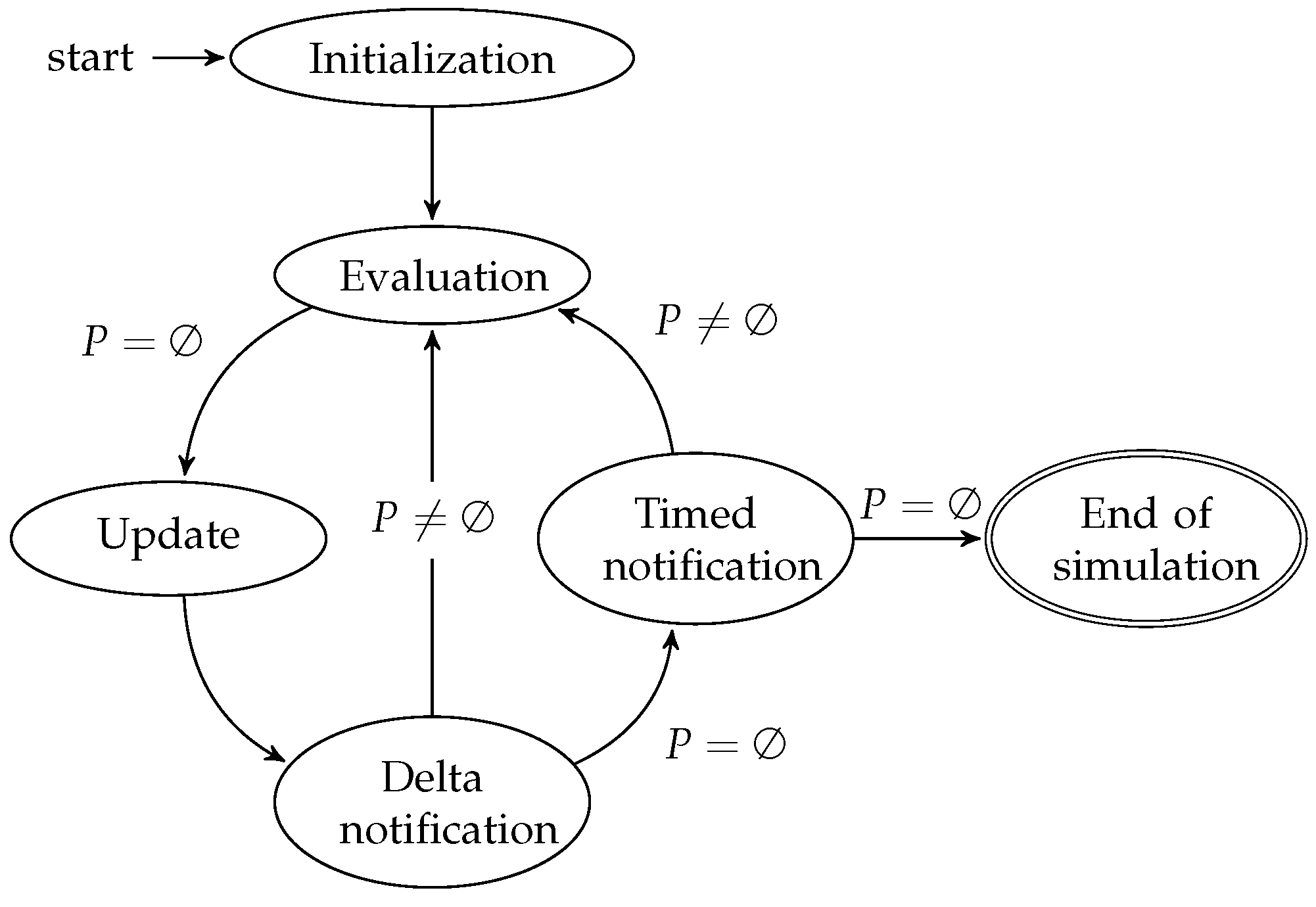
As a reminder, we first present in Figure 1 an abstract of the SystemC scheduler behavior, as stated in the SystemC standard [1].

The scheduler starts with an initialization phase that we do not detail here. In the evaluation phase, the runnable processes are started or resumed with no particular order. The immediate notifications produced by these transitions are then triggered. If there are runnable processes after the notifications, then the evaluation phase continues. Otherwise, the scheduler moves to the update phase, followed by the delta notification phase. The immediate notification loop is implicit on the figure, within the evaluation phase box. A delta cycle corresponds to the loop: evaluation, update and delta notification. At the end of a delta cycle, if there are no runnable processes, the scheduler checks timed events. If there are timed events, it picks the earliest one, sets the current simulation time to its time, and notifies the time change. A timed cycle corresponds to the loop: evaluation, update, delta notification and time notification. For concision we did not represent the other sets involved in the scheduling algorithm.

2.3. Time Modeling

In a TLM/LT model, the microarchitecture is not modeled, so the computation may be performed differently from the actual hardware, even if functionally equivalent. As a consequence, it makes no sense for a process to yield the control to another process in the middle of a computation: the state that the other process could observe would not be relevant with respect to the hardware [13,14]. Thus, a computation that takes time is usually modeled with a sequence like in Figure 2.

A construction commonly used in TLM/LT models is temporal decoupling. It has been added in the TLM-2 standard [15], but was in fact already used before in SystemC models. It consists in defining a local time for each process, which can be increased during the execution, getting ahead of the SystemC time. The increase is called a low cost timing annotation because it only operates on a local variable and induces no SystemC kernel operation. To keep time consistency, a time purge is defined. The purge of the local time happens notably when reaching synchronization points (synchronization-on-demand in TLM-2). This avoids synchronizing every time, but instead do the purge on essential events of the system. Then, using temporal decoupling, the sequence in Figure 2 becomes the one in Figure 3.

Precise timing information is not available in early models. Because of this, to avoid over-specification, time ranges are used in loosely timed models. The use of time ranges instead of time values changes the fact that two values (the bounds of the range) instead of one must be specified when annotating. For the synchronization, a value within the current time interval must be chosen, since the SystemC kernel needs a time value. The choice of the value within the range is implementation-defined. The current implementation in use at STMicroelectronics picks a random value within the interval. We will see in Section 5.3 that even if time ranges could be better used, the benefits in our test case are barely perceptible. This illustrates the claim we made in Section 1.

2.4. Communication Between SystemC Processes

In TLM the different processes are mostly communicating through TLM sockets. In practice, TLM sockets forward function calls from the source to the target until the final target is reached, where the function is defined. That means that a process emitting a transaction through a TLM socket will be executing a piece of code in the target module, i.e., which can use variables shared with other processes of the same module.

This is fundamentally different from sc_signal communication, which is the basic communication medium in cycle-accurate models. Indeed signals contain an isolation mechanism between their current value (i.e., the value returned by a read on the signal) and their future value (i.e., the value written to the signal). The future value is assigned to the current value during the update phase, but there is no race condition between a write and one or several reads during the execution phase (even if the execution semantics is relaxed to allow parallel execution during the execution phase). This isolation between readers and writers gives a convenient opportunity to have them running in parallel at negligible extra cost.

3. Problem Statement

The parallelization of LT SystemC/TLM simulations implies to solve several challenges. We do not present classic issues inherent to software parallelization, we focus instead on the ones induced specifically by such models, in particular in an industrial context.

A SystemC parallelization solution must not introduce race conditions. As stated in Section 2.4, in TLM models, communication is done by function calls, which involves shared resources. For example, two initiators (e.g., CPUs) that concurrently access the same target (e.g., a RAM) will concurrently call the same function of this target. That makes the target component itself a shared resource, introducing a race condition if not protected.

In the industry, there is a need to support heterogeneous simulations. That means that some parts of a model are designed with a different technology. For example, a vendor provided only the RTL model of a hardware block, but the rest of the model is written in SystemC/TLM. In this case, the RTL model can be simulated, or can be run in a FPGA device in co-simulation with the TLM model. One part of the model can even be a real hardware component (e.g., a prototype). An industrially compliant parallelization solution must be able to integrate this heterogeneity.

Another huge challenge for SystemC parallelization is the adaptability on existing platforms. Indeed, as for every technology change, the migration has a cost. This cost must be put in perspective with the time saved if the parallelization solution was in production: a solution that requires an important effort may not be profitable even if it shows substantial performance benefits.

To conclude with this section, we note a very important point regarding the conception of a parallelization technique: the knowledge of the profile of a simulation. Analogously, parallelizing huge independent computations on matrices is not performed the same way as parallelizing a shortest path algorithm. In our case, a simulation is mostly characterized by the model and not by the simulation kernel. In other words, a major interest in our research is to have the ability to characterize a simulation. One interesting measurement in that purpose is the number of runnable SystemC processes at each simulation cycle. Other ones include the wall-clock time consumption per transition, or per SystemC process. Both put in perspective, they give strong clues about the applicability of a parallelization option in a given case.

4. Profiling Method

We have developed a visualization and profiling tool called SycView. The motivations behind it are twofold:

• Finding a parallelization approach is through knowledge of the simulated models, as stated in the previous section. Thus, we need to get SystemC-aware measurements about the profile of a simulation.
• In an industrial context, it is frequent for complex models to be partially developed by external teams. This results in a large quantity of source code on which it is hard to have a comprehensive knowledge. We ease this aspect by taking a few steps back and giving an abstract view of a simulation.

4.1. Related Tools

We have found that most of the literature about SystemC visualization focus on the model description and architecture exploration. For example, the tools presented in [16,17,18,19] and more recently [20] gives access to the visualization of the hierarchical architecture of a platform, as well as the exploration of the components behavior. Such information is precious and these tools are complementary with our tool especially when it comes to understanding a design. However, what we found to be missing in these tools is a software point of view, in order to understand the model not as the representation of an SoC, but as a piece of software. Besides, some of the above mentioned tools need to instrument the model, which is generally not possible in the case of huge and complex models.

4.2. Presentation

The principle of SycView is simple: it consists in trace recording during simulation (Section 4.2.1) and then trace visualization (Section 4.2.2). In order to print traces, we instrumented the SystemC kernel, based on the ASI implementation. For the visualization we developed a graphical user interface written in Java, that takes the generated traces as input.

4.2.1. Trace Recording

The trace recording consists in printing data at interesting points. For instance, we print a trace each time a transition yields to the kernel, containing:

• The name of the SystemC process which triggered this transition.
• The type and arguments of the wait performed.
• The wall-clock time duration of the transition.

When the simulation ends, we store those information in text files. Then for example, we are able to find which SystemC process (or group of processes) globally consumes most of the time. Furthermore, we can use statistical metrics to get the average execution time of a process and compare it with the number of executions to highlight how each process spends its time.

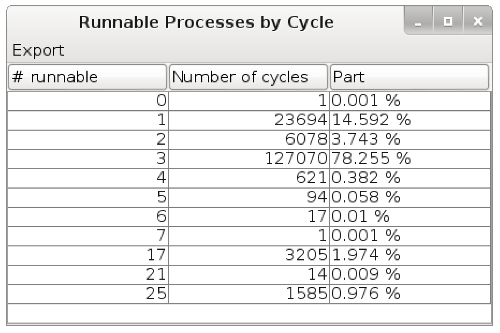
We also keep the number of runnable processes at the beginning of each simulation cycle. More precisely, what we get is the maximal number of runnable processes at the beginning of each immediate notification cycle within each delta cycle.

4.2.2. Visualization

We have implemented a graphical user interface providing six different views, which can be split in two main categories.

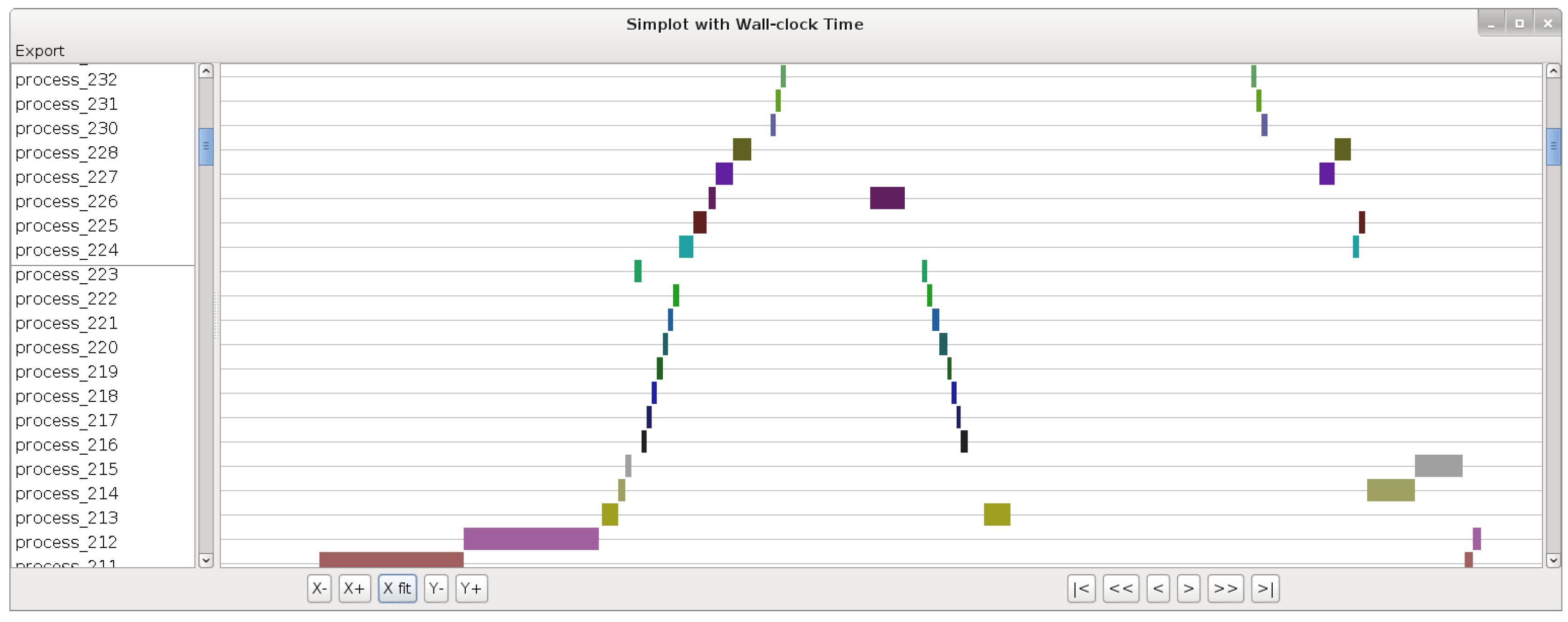
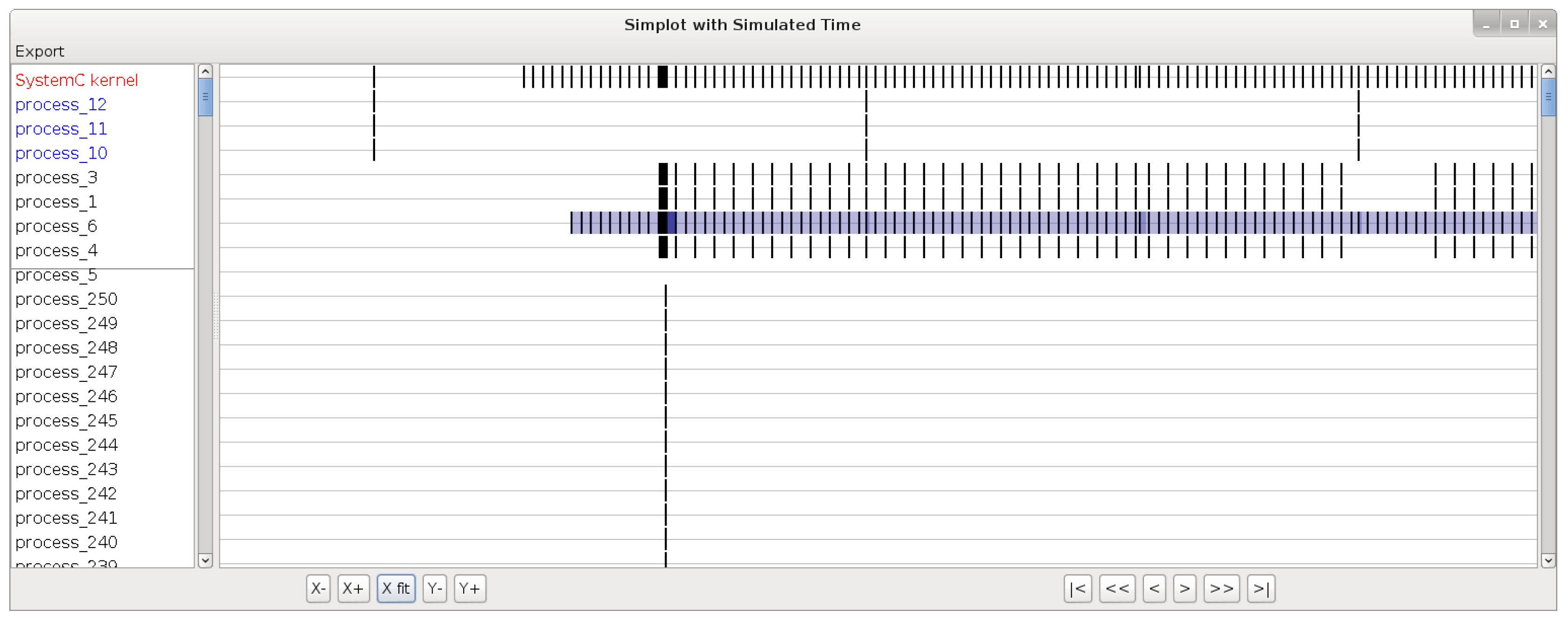
The first category is plotting the scenario of an execution (order and duration of transitions) as a function of either wall-clock time or simulated time. For example, Figure 4 shows the screenshot of a wall-clock time plot (for confidentiality reasons, the actual process names cannot be disclosed in this publication, hence process names are replaced with numbers in all figures). On this plot we can see that there seems to be a chain triggering of the processes executing in one order on the left part, and in the reverse order on the right part. The width of a rectangle is proportional to the wall-clock time duration of the corresponding SystemC transition. This view, as illustrated by this little example, can be used to identify patterns in the executions of transitions, and can highlight which transitions are particularly time-consuming. Such information could hardly be identified by a static code analysis, because of its complexity. On the other hand in Figure 5 we can see an example of a simulated-time plot. The processes are also represented on the left part, and on the right part, a vertical stroke is placed for each transition, in the simulated time it occurred. Note that what appears to be black rectangles are strokes close together. The blue rectangles represents time ranges in which the transition may have occurred, based on loosely timed information on the model. Note that time ranges are not part of the SystemC kernel so we added that when we instrumented the kernel because it was part of our industrial context.

The second category consists of giving statistical metrics about the platform execution. We display the wall-clock time consumption per process (with statistical metrics), as in Figure 6. We can see that the first process uses almost 13% of the time in 10111 transitions, while the third process uses almost 8% of the time in only 14 transitions. That makes a huge difference in the mean execution time, and we can deduce that optimizing the third process may be more efficient than the first one. 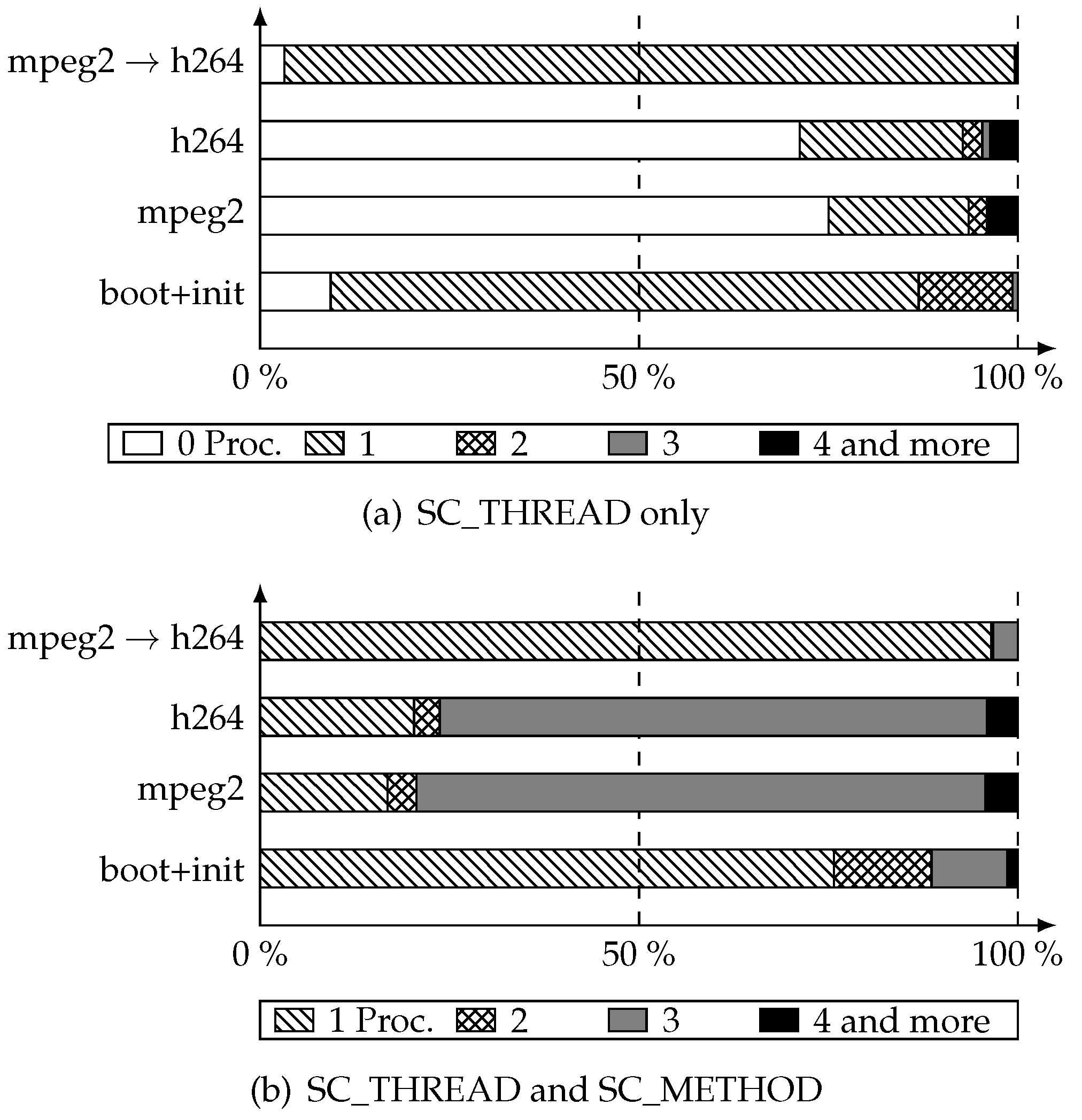Moreover, we show the number of runnable SystemC processes at each delta cycle, shown in Figure 7. This table can also be displayed for SC_THREADs or SC_METHODs only.

5. Results

In this section we present the results of SycView for the simulation of an industrial case study, which is the model of a set-top box including video encoding/decoding. The software running on it is a modified Linux kernel.

5.1. Overview

The platform has one CPU containing four general purpose cores. One important aspect about this platform is that most of the computations are not performed in the software but by hardware acceleration blocks.

This model is composed of $\sim 900,000$ lines of code including $\sim 750,000$ lines of C++ code (given by cloc). It contains 850 modules hierarchically organized. Counting only the leaf modules leads to the number of 750 modules. There are 1068 registered SC_THREAD and 163 SC_METHOD.

5.2. Number of Runnable Processes per Cycle

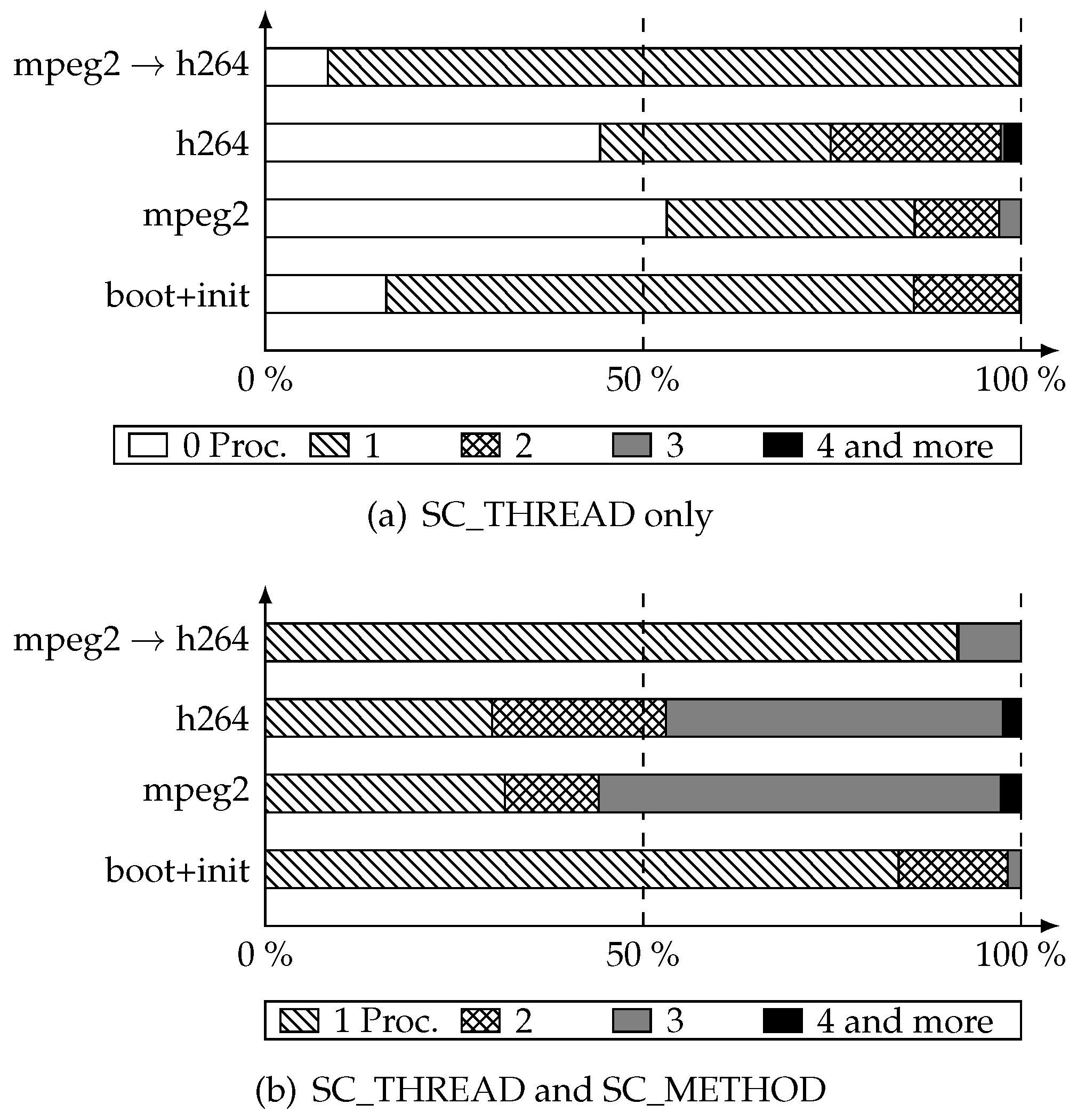
In this part we present the measurements of the number of runnable processes at each cycle, performed by SycView (cf. Figure 7, however, for clarity we will show these results on charts). Different test scenarios have been experimented. The first one is the boot and initialization of the platform, which starts in the beginning of the simulation and ends when a command shell is available (let us remind that a Linux kernel is running on the model). All the following scenarios start after the boot and initialization. The two following cases display video broadcast tests for h264- and mpeg2-encoded streams. They consist in providing an encoded video stream as platform input. The video stream is decoded by hardware blocks and sent for display. The last case is a transcoding, which redirects the decoded video stream to encoding hardware blocks in order to produce a h264-encoded stream from a mpeg2-encoded stream.

In Figure 8 are shown the measurements. Figure 8a shows the number of runnable SC_THREAD at each simulation cycle. Let us analyze, as an example, the case of mpeg2 video display. For 53 percent of the cycles, there were no SC_THREADs to run (i.e., only SC_METHODs). For 32 percent of the cycles, there were one runnable thread. For 12 percent there were two runnable threads and finally for the remaining 3 percent there were three threads to run. The h264 case showed the same trend. For the transcoding case, most of the cycles only had one thread to execute. On Figure 8b are shown the measurements for all processes. The big picture here is that the huge majority of simulation cycles only execute one to three transitions before moving to the next one.

A notable point is that this measurement gives an upper bound of the degree of parallelization achievable with parallelization inside cycles (detailed on Part 6.1). Due to shared resources, the real degree of parallelization may be lower than this upper bound. Indeed a runnable process may share a dependency with another one, making the concurrent run of those two processes not consistent with coroutine semantics.

5.3. Influence of Randomized Waits on Number of Processes per Cycle

As we have seen in the previous section, the number of runnable processes at the beginning of each delta cycle is too low to expect an interesting speed-up with parallelization inside delta cycles for such platforms. The fact that the number of processes ran during each cycle is low can be explained by at least two factors:

• The platforms are described at a high abstraction level where both the time and space granularity are coarse: instead of modeling the behavior of small pieces of circuit at each clock cycle as done in RTL, we model the overall behavior of components avoiding the wait statement. The coarse space granularity leads to fewer processes than RTL. Since we do not model hardware clocks in LT, the chances of simultaneous execution of multiple processes is reduced.
• Since our implementation of loose-timing uses randomized wait statements as presented in Section 2.3, the probability of having two processes waking up at the same instant is reduced. For example, even two processes executing the exact same code will not be temporally synchronized if they used randomized timing.

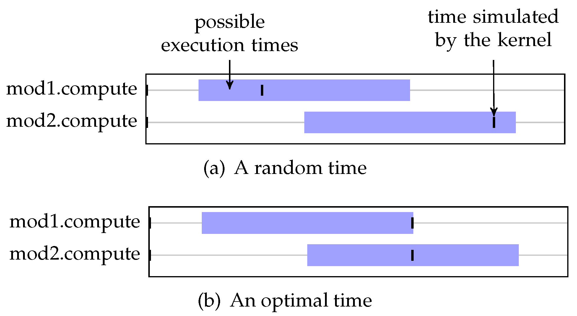
Point 1 is intrinsic to the way we describe the platforms, but point 2 is a side effect of the implementation of loose-timing. By changing the implementation, we can actually take advantage of loose-timing: since the times are chosen arbitrarily in an interval, the implementation can pick the one that will maximize parallelism instead of choosing one at random. This section describes such implementation and the results on our case-study. We show that the benefit is actually very low, which leads to the conclusion that point 1 is actually the main reason for the low number of processes within each cycle.

In its current form, the optimization can be implemented neither in the loose-timing API (which does not have visibility on the number of processes eligible at a certain date) nor in SystemC (which is currently called through wait after the random duration is chosen). To exploit ranged timing annotations, we have added this function to the SystemC kernel:

void wait(sc_time min, sc_time max);

This function has the following semantics: yield to the kernel, and wake up the current thread on a time included in the given range. To illustrate how we choose the best value in order to maximize the number of runnable processes in the next delta cycle, we present an example. Let us consider the following code in two distinct SC_THREAD that we consider independent from each other:

void mod1::compute() {

• // ...
• wait(sc_time(1, SC_NS), sc_time(5, SC_NS));
• // ...

}

void mod2::compute() {

• // ...
• wait(sc_time(3, SC_NS), sc_time(7, SC_NS));
• // ...

}

A graphical representation of executions of this model is shown on Figure 9. We can see the processes (on the left side) and rectangles (on the middle part) which indicates the time interval in which the execution of the corresponding process is valid. The times actually simulated by the simulator are represented by dashes.

With this representation, it clearly appears that depending on the times that are simulated, we have a different number of runnable processes on a different number of cycles:

• In the case of Figure 9a, there are two simulated times, each with one runnable process.
• In the case of Figure 9b, there is only one simulated time, with two runnable processes. Thus this case induces a higher degree of parallelization for an approach inside delta cycles.

To implement such a strategy, we had to bind STMicroelectronics’ annotate/synchronize API (see Section 2) with this newly added wait. The computation of the simulated time is no longer performed in the synchronize method, but is dedicated to the modified SystemC kernel. Finally, the last part is to implement a policy to choose the next time to simulate, in the kernel. To choose the next simulated time value, we choose the minimum value of all the upper bounds, for all the registered time events. By choosing the minimum value of all the upper bounds, we guarantee that the next time is not too late (i.e., that we do not skip any registered timed event). Moreover, it is the farthest valid time, so it will trigger the biggest number of processes, for the next time cycle. Then each timed event whose range includes this value is popped and triggered. Note that with this strategy, we are still compatible with the old wait by defining a time range with both bounds equal to the same time value.

By implementing this policy, we maximize the number of runnable processes at the beginning of each cycle for an execution. The final purpose is to determine if this maximized value is high enough to justify the use of parallelization inside delta cycles techniques. We have run again the simulations of our industrial platform for the same test cases to measure the same metrics with this improvement. In Figure 10, we see that, in most cases, the number of processes is still very low, even if in we have more occurrences of cycles with 3 and 4 or more runnable processes.

Those results illustrate our point: parallelization inside delta cycles will not efficiently parallelize the simulation of such models, even after performing a non-trivial optimization and even ignoring race condition issues. Indeed, the maximum speed-up achievable is no more than 4 (which is actually a very optimistic bound).

5.4. Wall-Clock Duration

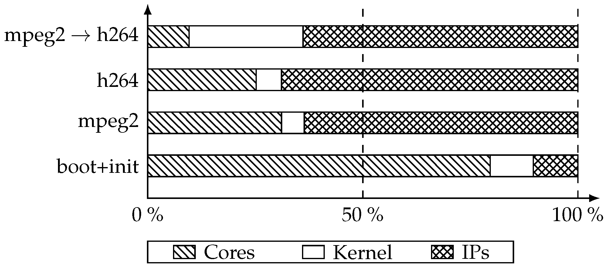
In this section we show the wall-clock time consumption per SystemC process (cf. Figure 6). As an overview result, Figure 11 presents the distribution of wall-clock time between three different categories:

• processes from CPU core models (Cores)
• processes from hardware block models (IPs)
• SystemC kernel (Kernel)

For the boot and initialization case, 79 percent of the time was spent in core models, leaving 10 percent in hardware blocks and the remainder in the SystemC kernel. The explanation here is rather straightforward: the system boot is performed by the CPU and is not hardware accelerated. In the video stream decoding cases (both h264 and mpeg2), one third of the time (respectively 25 and 31 percent) was spent in cores and the rest was mostly spent in hardware blocks. Note that the time spent by the SystemC kernel is above 6 percent. This illustrates that the decoding computations are mostly done by hardware IPs. Finally, for the transcoding case, 10 percent of the time was spent on the core, 25 percent on the SystemC kernel and 65 percent on hardware IPs. Again, we notice that hardware blocks are performing most of the computations, even if in this case there seems to be an overhead on the SystemC kernel, due to a high number of synchronizations in hardware blocks specifically triggered during this test case.

To get into more details, we present in

Table 1. Measurements of wall-clock time consumption for the four most consuming processes. Min, median and max corresponds to the execution time of transitions. For confidentiality reasons, we did not show the SystemC names of those processes, but only their category (hardware, core or kernel).

Category	Type	Part	Nb. Transitions	Min (μs)	Median (μs)	Max (μs)
Hardware block	SC_THREAD	12.9%	10,111	> 0	1,123	18,372
Hardware block	SC_THREAD	8.6%	93	73,652	77,535	84,082
Hardware block	SC_THREAD	8.0%	14	395,202	486,617	495,737
SystemC kernel	-	5.9%	635,129	> 0	> 0	983

the results for the four most time consuming SystemC processes in the test case h264. More than 35 percent of the total time was spent on those processes. However, if we look at the number of transitions, we see that the first process (part of the IPs category) consumed 12.9 percent of the total time in 10,111 transitions while on the other hand, the second and third processes (also IPs) performed considerably less transitions (less than 100) but still consumed around 8 percent of the time each. This means that transitions of the second and third processes are performing long computations, while transitions of the first process are short in comparison. This is confirmed by the minimum, maximum and median execution times for those processes’ transitions. The fourth one is the time spent in the SystemC kernel.

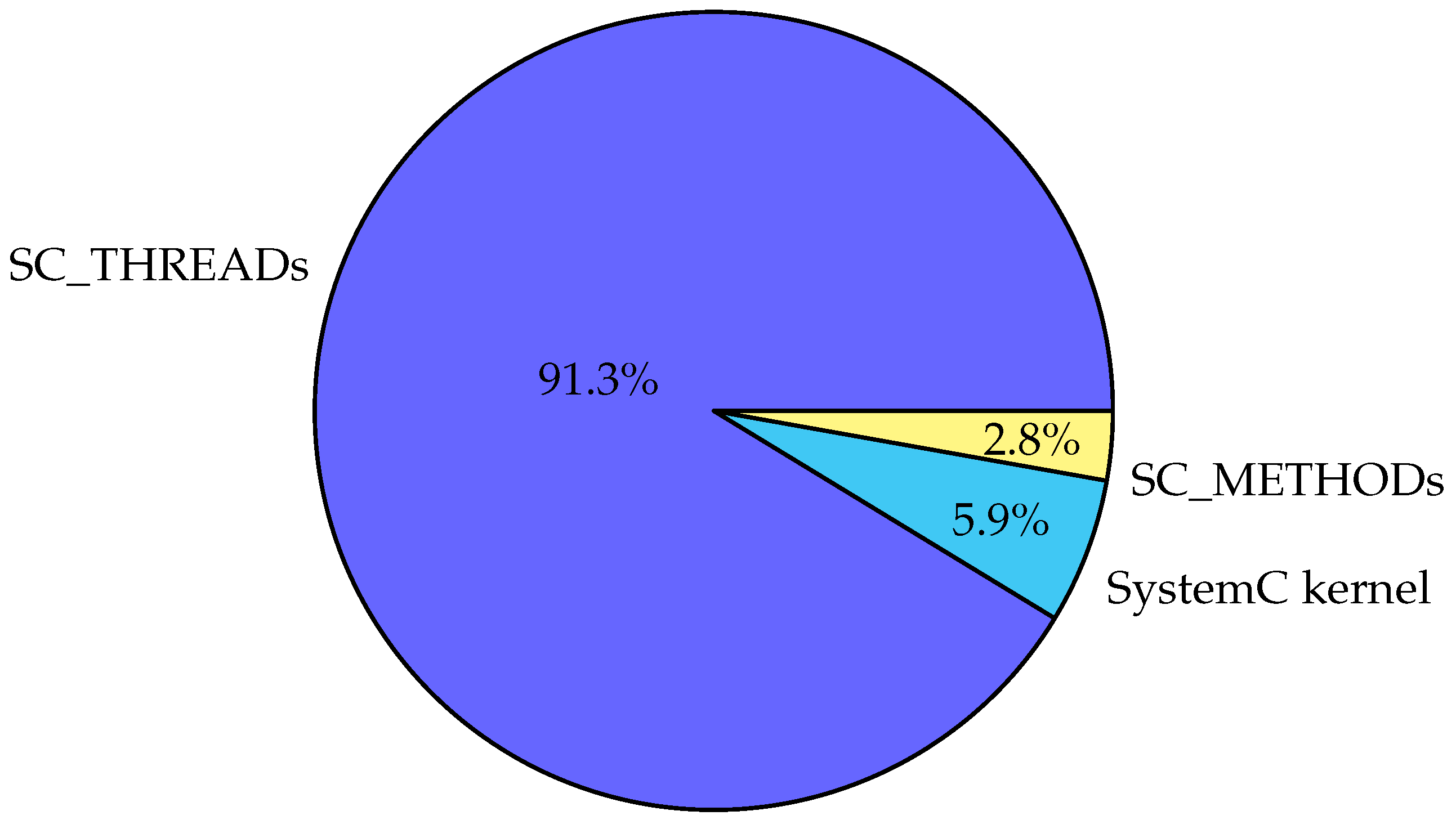
Finally, we present the time consumption per type of process (thread, method or kernel) in Figure 12. Rather predictably, a huge proportion of the time, namely 91.3 percent, was spent in SC_THREADs. However, this result may be put in perspective with the previous ones, especially with the number of runnable processes. We have seen in Figure 8a that there were a considerable number of cycles with no SC_THREAD to run. Still, most of the time is spent in their transitions.

5.5. Summary

In summary, the characteristics of our case study are:

• Most of the wall-clock time is spent on hardware block models, not on CPU models (Figure 11).
• Most of the wall-clock time is spent on SC_THREADS (Figure 12).
• Most of the simulation cycles have less than four runnable SystemC processes (Figure 8) and even if we exploit time ranges to maximize this value (Figure 9), the results remains similar (Figure 10).
• In the cycles where there are several runnable processes to run, most of the time there is zero or one SC_THREAD, the remaining being SC_METHODs (Figure 8 and Figure 10). The wall-clock time consumed by these SC_METHODs is very low compared to the time consumed by the SC_THREAD (Figure 12).

Obviously, the above characteristics may vary depending on the test scenario. However, they have been observed for the most common uses of a set-top box model, i.e., video display tests.

6. Existing Parallelization Approaches

This section reviews existing approaches for SystemC program parallelization. For each of them, we discuss the applicability on our case study, keeping in mind the results of measurements obtained in the previous section.

6.1. Parallelization Inside Cycles

A conservative PDES simulator with lookahead has been implemented in [21]. The solution works on top of the SystemC kernel, which remains unchanged. To apply this solution, the model must be written in compliance with some provided templates. It explicitly targets RTL-like platforms, because the solution is based on low-level SystemC features like sc_signal, which tends to be unused in TLM models. This proposal comes with a lot of future work propositions, and is not industrially applicable as-is. Some of the proposed ideas are addressed by more recent papers.

The works presented in [2,3,5,22] use the fact that within a delta cycle, the execution order of the processes is undefined. The approach goes one step further: since the correction of the SystemC program should not depend on the execution order, it should, in most cases, not be broken by a parallel execution within a cycle. A synchronization barrier is placed at the end of each delta cycle. The processes are partitioned into groups that will be executed by an instance of the SystemC simulator on a specific core. In [5] all the processes of a module have the same affinity. In [2] the authors have experimented different strategies to balance the load on the available cores. Finally, in [22] a technique is proposed to solve the problem of race conditions introduced by TLM interface method calls by adding a split point in transactions and moving the caller thread into the target group.

In [23] an analysis of the execution semantics of both SystemC and SpecC is presented. The authors have implemented an extension to the SpecC simulation kernel to support multi-core simulation. However, the semantics of SystemC and SpecC are different, notably in their definition of signals. In SpecC, signals are defined as monitors: each of their accessors/mutators are in mutual exclusion. Moreover, as stated in Section 2.4, there is a real difference between cycle-accurate modeling using sc_signal and TLM modeling using sockets. In the first case, the built-in isolation offers a good opportunity for parallelization. In the second case, the race condition problem induced by function calls must be solved differently.

A high degree of parallelization can be achieved by exploiting GPUs. This has been studied by [4,24,25]. In [4,25] the authors have chosen to use CUDA (Compute Unified Device Architecture). The proposed tool in [4] is a source-to-source translator which produces a CUDA-style code from a RTL-synthesizable SystemC model. High speed-ups are achieved, nonetheless we can notice that all the test cases are pipelined platforms at RTL level. In [24] the authors compared a CUDA and an OpenCL implementation. The work presented in [25] consists of exploiting both GPU and multi-CPU architectures. It supports mixed-abstraction simulations. The parallelization is performed within delta cycles, with support for immediately notified processes. They have benched their solution on a set-top box model, which was implemented in order to be used as a bench. This induces that some optimization have been made, that may hide the real amount of refactoring needed to efficiently parallelize an existing industrial platform.

In [26] is presented the RAVES hardware platform. Each evaluation phase is parallelized (i.e., even after immediate notifications). Though, the new aspect here is that the authors have implemented a hardware architecture which implements their parallel SystemC kernel, and the actual embedded software running on it is the platform model. The results are promising, but their test cases are cycle-accurate models of many-core platforms.

Finally, a parallel implementation of SystemCASS, a cycle accurate version of SystemC, is presented in [27]. The authors have implemented a SystemCASS simulator that executes all the transitions (Mealy or Moore) of the same cycle in parallel.

As a conclusion of this subsection, we can notice that due to the chosen approach, most of the SystemC simulator instances are in the same delta cycle, or at least the same time cycle. Thus, it clearly appears that a necessary condition to have a significant speed-up is to have a sufficient number of concurrently runnable processes in the most wall-clock time consuming cycles. We showed in Section 5 that this is not the case in our example platform. Due to the TLM/LT modeling style and the architecture of the platform (complex computation performed by hardware acceleration blocks) we can reasonably assume that the situation will be the same for other similar models.

6.2. Dependency Analysis

The SystemC standard states that within a delta cycle, the execution order of the processes is undefined. That does not mean that they can be run concurrently as-is, because the next sentence explains that in order to do so, one must analyze the dependencies between processes to prevent race conditions. Indeed, one must consider the case of shared memory and/or resources. To solve this problem, most of the work presented in the previous section have chosen either to make strong hypothesis about the model or to ask the model developer to protect critical sections manually. On existing platforms, it happens that most of the time the manual refactoring is excluded, and the hypothesis are not fulfilled. To automate the prevention of race condition, static or dynamic dependency analysis can be performed on the model.

In [28] is presented a parallel SystemC simulator with static analysis of dependencies. A static analysis tool first scans the model in order to produce a dependency scheme. Then this dependency scheme is provided as input to the modified SystemC simulator, which uses it to schedule in parallel different processes. The main idea is that a runnable process can be run if it is independent with each running process. As presented in Section 3, the case where multiple components perform a transaction to the same target is equivalent to a shared resource access. However, the static analysis presented here does not include transaction address resolving.

Following [23], in [29] the authors present a simulator which performs static analysis to prevent data, timing or event conflicts. The technique is similar to branch prediction in hardware. The parallelization is performed within delta cycles.

The solution presented in [30] uses both static and dynamic analysis to propose an adaptive algorithm and tool flow for SystemC/RTL parallelization. Their current solution is based on RTL features, e.g., sc_signal, but they used a sufficient level of abstraction in their algorithm to keep hope for future TLM support (planned as a future work by the authors).

Most of these approaches parallelize inside cycles, so we still have the same issue with efficiency as in the previous subsection. Moreover, performing static analysis on industrial size models as-is can be excluded because of the code complexity.

6.3. Distributed Time/Relaxing Synchronizations

In [6] a programming paradigm for many-cores and many-clusters modeling in SystemC is presented. The work is based on the PDES principle and proposes a conservative synchronization with a lookahead time. Multiple instances of a SystemC simulator are run. To avoid deadlocks, the sending of null messages (which only contains a timestamp) is introduced. The handling of interrupts is proposed by the addition of a timestamp to it, with a polling in the beginning of each CPU loop. This removes the asynchronous characteristic of interruptions, but guarantees that they will be noticed in a meaningful time. Their test bench consists in comparing a CABA (Cycle Accurate Bit Accurate) simulation to a TLM one, in order to balance the time saving with the loss of precision. The conclusion of their work is that for a very acceptable loss of precision, they can simulate models at TLM speed, so approximately 50 times faster than for CABA simulations. However, we can identify two major drawbacks in their bench. The first one is that the software task is very basic: wait for an interrupt and then display a message on the terminal, in a loop. The second one is that the best speedup is reached for the platform with the biggest number of simulated cores (i.e., 39). On our industrial platform, the number of simulated cores is low (no more than 7) and the software is more complex. The next work completes this one by proposing an implementation of this simulator: TLM-DT (Distributed Time).

TLM-DT is presented in [7,31]. It is compliant with the TLM2 standard, but it needs to shift from a global time to a distributed time, which induces to modify all the timing information in the model. This solution reaches good performances on many-core SoC and NoC (Network-on-Chip) platforms, composed of many instances of similar if not identical components. This regularity in the architecture induces a different profile from platforms with several different hardware acceleration blocks.

To apply this solution, one must first adapt the platform code to fit TLM-DT API. We can also point out that it targets many-core SoC or NoC models. This provides the hypothesis that most of the simulation time is spent on the numerous similar CPU/core models. In our case study though, we have seen that most of the time is spent on hardware modules.

Based on TLM-DT, the authors of [8,32] have developed their own parallel implementation of a SystemC/TLM simulator. It is based on a PDES algorithm and designed for clustered platforms. Both implicit and explicit synchronizations have been implemented to bound temporal errors. Their analysis is common to SystemC and SpecC languages. They particularly focus on protecting the shared parts of the simulation, i.e., the simulation kernel and the communications, and have included locks in their scheduling algorithm. They present promising results on hardware-parallelized versions of video decoding and image encoding models.

An optimistic approach of PDES has been studied in [9]. The optimistic characteristic does not come from a rollback mechanism (contrary to what optimistic means in other research papers) but from a weak synchronization mechanism. The platform is divided into groups of modules, which are simulated by a specific instance of a SystemC simulator. Synchronizations are performed when a time quantum has been overlapped. It is also possible to define transaction-specific time behavior. This approach makes strong hypothesis about shared variables: it considers that shared variables (except the ones from the SystemC kernel) has been either well protected or purposely not protected.

In [10,33] a parallel SystemC simulator implementation called SCope is proposed. The idea is to run different processor models on separate simulator instances. Each instance has direct access to some objects of the simulation (i.e., modules, ports, threads, etc). Simulator instances are allowed to run at different simulation times: a lookahead time is defined. Their results showed a good speed-up on a four-cores host, for the model of a specific hardware structure called EURETILE which is similar to a network-on-chip.

In [34], CoMix, a concurrent model interface for distributed simulation, is presented. The principle is similar but is not limited to the processor models. The platform is cut into parts that do not have to fit the SystemC hierarchy, however this implies a structural refactoring on the model. Then every partition is bound to a connector in charge of delivering communication at the right time. The different parts are allowed to run at different simulation times, provided they are in the same time quantum. Nonetheless, a strong hypothesis made in this work is that models are composed of many processors, tens or hundreds of them. That means that the modeled systems are more software-oriented than hardware-accelerated, both having very different execution profiles.

More recently, SCale has been proposed in [35]. It is a parallel simulation kernel designed to speed up the simulations of many-core architectures. Basically, it consists in having a parallel evaluation phase. The different SystemC processes are manually attributed to worker threads. The authors have taken care of the reproducibility by adding a replay mechanism based on the saving of the scheduling on a file. We can notice that because of our results (Figure 8) parallelizing only the evaluation phase will not be efficient. Still, temporal decoupling could be used to increase the cycle parallelism. However, in our case the experiments (Figure 10) revealed that exploiting simply time decoupling will not significantly increase the degree of cycle parallelism.

Finally, in [36], SystemC-Link, a simulation framework for SystemC simulators, is presented. It is an overlay above SystemC kernels, which allows the use of different versions of a SystemC kernel in one simulation. An existing model must be partitioned into segments, each one run on a different simulator. Then, the framework’s task is to link the simulators and keep them synchronized. Again, the efficacy depends on temporal decoupling. This makes the approach best fit for cycle-accurate models, with precise timing, where relaxing temporal constraints removes more constraints than in LT models.

6.4. Tasks with Duration

In [37] the authors present jTLM. This is a Java experimentation framework for TLM simulation. The interest is that it can exploit multi-core architectures, by introducing a different timing approach: tasks with duration, as alternative to instantaneous computations followed by a time elapse. This notion has been extended in a SystemC framework called sc_during [12]. The idea is to change sequences like:

void thread() { // declared as SC_THREAD

• compute();
• wait(time);

}

into:

void thread() { // declared as SC_THREAD

• during(time, compute);

}

Now, a duration is associated with a task. Semantically, this means that the during task can be executed in parallel with the rest of the simulation. Indeed, if a during task is run at time T, for a duration D, it means that the task computation can be executed at time T, at time T + D or at any time between T and T + D. This implies that there is no dependency between the task and the rest of the platform within the interval [T; T + D] and so that it is safe to run the task in parallel.

In the case of sc_during the amount of refactoring needed is debatable. This solution needs some refactoring in the code of the platform to actually parallelize it, but it has the advantage to let legacy SystemC code running as-is, sequentially. That makes this solution relevant for platforms where wall-clock time consuming parts can be clearly identified, and are present in sufficient number to justify the parallelization. This solution explicitly targets LT models; the notion of tasks with duration is not meaningful for clock sensitive processes.

To conclude with sc_during, we add that it is possible to synchronize a during task with the SystemC kernel. For example, the duration of the task can be extended, or a SystemC primitive can be called. However, in the latter case, there is a major overhead because the two threads (the one executing the kernel, and the one executing the task) must synchronize with each other. So even if this is possible, too frequent synchronizations will induce a dramatic slowness in the simulation.

6.5. TLM without SystemC

The authors of [38,39] present a parallel TLM simulation kernel not based on a SystemC layer. This removes the plurality of modeling levels enabled by SystemC, but allows fine optimization. The authors have implemented a dynamic load balancing strategy to compute the number of simulator instances to run, and the amount of tasks to give to each one.

7. Conclusions

Research on the parallelization of SystemC simulations has already produced different tools, and many of them allow important performance and scalability improvements. However, in this paper we showed that the case of LT SystemC/TLM models with few cores and hardware IPs raises a lot of different challenges not addressed in previous work. LT models are the only option for very fast simulation at an early stage of the design flow: they provide very good sequential performance by abstracting details that would slow down the simulation, require lightweight modeling effort and do not require information about detailed microarchitecture that are not yet available at this stage.

We showed that LT models exhibit characteristics that prevent most parallelization approaches from working. Approaches that run processes in parallel within delta cycles cannot get a speed-up greater than the number of processes runnable in this cycle, which hardly reaches four in our case. Besides, many approaches consider that the SystemC processes must not share variables, which is not true for TLM/LT because of the communication through function calls. As a consequence, most existing approaches are fundamentally limited when it comes to LT models. Some approaches tackle the problems specific to LT models. For example, sc_during [12] was designed to allow parallelization across delta cycles and to require a minimal refactoring effort. Still, the trade-off between the amount of refactoring and the speedup is difficult to find. Our preliminary experiments with sc_during on the case study did not show significant speedup. The approaches in [22,34] are designed to parallelize LT models as well. However, some aspects about the semantics (e.g., adding a split point in transactions) or the efficiency (e.g., finding the best partitioning of a model for distributed simulation) are still to clarify.

We believe that this paper provides a better understanding of the problem. By providing some measurements on an industrial platform, we even quantified the issue. We hope that these experiments will help new approaches to emerge and to be experimented on representative benchmarks. In future works sc_during can be tested on such industrial platforms to evaluate the benefits and balance it with the amount of refactoring. Moreover, temporal decoupling can be exploited better to reduce the synchronization needs between components.