Article

Dependable Control for Wireless Distributed Control Systems

1
Electronics & Control Group, Teesside University, Middlesbrough, TS1 3BA, UK
2
Department of Electrical Engineering, University of Faisalabad, NFC-IEFR Faisalabad, Pakistan
*
Author to whom correspondence should be addressed.
Electronics 2015, 4(4), 857-878; https://doi.org/10.3390/electronics4040857
Submission received: 27 June 2015 / Revised: 21 October 2015 / Accepted: 24 October 2015 / Published: 2 November 2015
(This article belongs to the Special Issue Wireless Sensor and Actuator Networks)

Abstract

:
The use of wireless communications for real-time control applications poses several problems related to the comparatively low reliability of the communication channels. This paper is concerned with adaptive and predictive application-level strategies for ameliorating the effects of packet losses and burst errors in industrial sampled-data Distributed Control Systems (DCSs), which are implemented via one or more wireless and/or wired links, possibly spanning multiple hops. The paper describes an adaptive compensator that reconstructs the best estimates (in a least squares sense) of a sequence of one or more missing sensor node data packets in the controller node. At each sample time, the controller node calculates the current control, and a prediction of future controls to apply over a short time horizon; these controls are forwarded to the actuator node every sample time step. A simple design method for a digital Proportional Integral Derivative (PID)-like adaptive controller is also described for use in the controller node. Together these mechanisms give robustness to packet losses around the control loop; in addition, the majority of the computational overhead resides in the controller node. An implementation of the proposed techniques is applied to a case study using a Hardware in the Loop (HIL) test facility, and favorable results (in terms of both performance and computational overheads) are found when compared to an existing robust control method for a DCS experiencing artificially induced burst errors.

1. Introduction

The use of wireless communication systems in automation and real-time control applications is increasing at a steady rate. Wireless systems have the distinct advantage of reducing equipment installation complexity through the lack of a need for wiring and harnessing, enabling easier trouble-shooting and system re-configuration; this reduces the long-term maintenance requirements associated with wired systems [1,2,3,4]. In addition, wireless sensor/actuator networks (WSANs) can potentially provide the device interconnectivity needed for a range of industrial control and monitoring functions across a wide range of operating environments [1,2,3,4]. However, wireless systems are generally perceived in a negative sense for real-time and safety-related applications such as the sensor/actuator networks needed for industrial process control systems [5,6,7]. The use of wireless technologies in these applications poses several severe problems, which include out-of-order packet transmissions, high levels of packet jitter and high probabilities of packet losses; these problems are especially problematic in systems with strict timing constraints [4,5,6,7]. Although much progress has been made in recent years, to date most industrial applications of wireless technology have mainly been restricted to soft real-time process monitoring and data acquisition applications, in which interruptions to the wireless service do not lead to unacceptable loss of control or damage to equipment [4,7]. When control loops have been closed by wireless equipment in industrial situations, developers have often been forced to take drastic actions; for example the enforcement of “blackout zones” around the feedback control loops in question [7]. Indeed, as discussed by [4] and [7], the use of wireless technology in feedback control applications presents arguably the largest ongoing challenge in the domain, and is the focus of the current paper.
The particular structure of WSAN architecture under consideration is as depicted in Figure 1, which is common in many industrial situations [1,2,4,7,8,9]. In such a system, a distributed “sensor” node samples and processes the controlled variable, and communicates this information to a “central controller” node for control signal calculation. The controller communicates the control signal to a distributed “actuator” node for final processing and application of the controls to the plant manipulated variable. Although not explicitly indicated in the figure below, we assume that a wired network (typically Ethernet based) may also be present between the wireless interface and the central controller node. In addition, although again not explicitly indicated, we assume that the paths between sensor-controller and controller-actuator nodes may consist of multiple hops which are possibly routed through more than one bridged LAN. This would be a typical arrangement for a Distributed Control System (DCS) for an industrial plant. No specific assumptions are made regarding the operation principle of the underlying wired and wireless networks or as to whether the underlying protocol(s) are of the decentralized (Multi-Master) or centralized (Master-Slave) type, but it is well suited to either (i) a flexible TDMA scheme with polled Media Access Control (MAC) and support for retransmission in case of detected errors (e.g., see [8,9,10,11,12,13]) which many industrial networks are based upon or (ii) a non-specialized architecture such as WiFi, along with a protocol such as sNTP (simple Network Time Protocol) for node clock synchronization.
Figure 1. Wireless sensor/actuator network (WSAN)-based Control System.
Electronics 04 00857 g001
In this paper, the concern is with ameliorating the effects of sensor and controller packet losses in such a sampled-data Distributed Control System (DCS). Such packet losses present as temporary interruptions to the inter-node information flows in Figure 1. The techniques described in this paper provide extensions to earlier techniques developed by the authors [14], which overcome some of the deficiencies identified in the previous work. Specifically, these deficiencies included: (i) an assumption that a nominal model of the process under control is available; (ii) the process under control does not experience unmeasured disturbances during operation; (iii) the dynamics of the process under control are assumed time-invariant with known parameters and (iv) packet losses are not experienced between the controller and actuator nodes. In particular, the contributions of this paper are to extend the work of [14] to develop and test an adaptive compensator for feedback packet losses to help overcome limitations (i)–(iii), and to also introduce a predictive buffering mechanism to help overcome limitation (iv). In addition, we also describe a simple automatic controller tuning method, which uses the plant parameter estimates obtained from the adaptive compensator to calculate a robust Proportional Integral Derivative (PID)-like pole-placement controller. The overall method is applied to a servomotor example using a prototype Hardware-In-The-Loop (HIL) test facility to illustrate its effectiveness. The results obtained are contrasted with a buffering scheme using a frequency domain robust control design technique to compensate for packet losses, and shown to compare favorably.
The compensator and buffering mechanism are based around a recursively updated Controlled Auto Regressive Integrated Moving Average (CARIMA) process model. The model provides predictions of the process state which include the effects of unmeasured disturbances, which are used to reconstruct estimates of a sequence of one or more missing data samples using a time history of successfully received process data. The model is also employed to recursively calculate future control actions (either using our suggested adaptive control law, or for any arbitrary causal control law) to enable the buffering technique. Under the assumption that a suitably rich time history of data has been available, the estimates will be optimal in the least squares sense, and the future calculated control moves will be (open-loop) optimal. Together, this affords the system a great deal of resilience against packet losses.
The remainder of the article is organized as follows. Section 2 reviews some previous work in this area, while Section 3 states some assumptions. Section 4 presents the main descriptions of the proposed adaptive compensator for sensor packets, while Section 5 presents details of the proposed predictive buffering mechanism for control packets and the adaptive controller design. A prototype HIL test facility to test an implementation of the proposed techniques in a small WSAN is described in Section 6, and a case study and experimental results are discussed in this Section. After a short discussion, the paper is concluded in Section 7.

2. Related Work

2.1. Wireless Networks for Industrial Control

Real-time control systems are often best designed around time-triggered (TT) principles due to their periodic nature and the requirements for low sampling and actuation jitter [15]. In WSANs, hybrid (or flexible) variations on TT behavior have found to better suited than strict TDMA [8,9,10,11,12]. The most existing wireless protocols for industrial applications (such as WirelessHART and ISA 100.11a) employ TT-based schemes [4]. At this stage, it is also worth acknowledging that there has also been recent interest in event-based triggering in WSANs, such as variations on the “Send-On-Delta” strategy [16]. However, such event-based schemes are not directly considered further in this paper as they only provide extremely limited facilities for fault tolerance (an implicit assumption is that a packet omission indicates that the measured variable has not changed by a magnitude greater than a pre-specified bound [16]). Additionally, they can experience excessive jitter during worst-case scenarios [14], and will normally default to loose time-triggering behavior anyway during process steady-states through the use of timeout mechanisms [16,17]. Although TT-based systems have been found effective to help reduce levels of packet jitter, the effects of packet loss and channel dropout still required special consideration. In wired networks such as CAN, Bit Error Rates (BERs) may be in the region of 10−6, normally arriving in short correlated bursts of approximately 5–20 bits [18]. As such, packet loss probability in these situations is comparatively low, and the omission of multiple consecutive samples can effectively be considered to be a “rare” event. However the nature of a wireless channel is such that packet loss probabilities are comparatively higher, and—importantly—will typically be strongly correlated [3,8,19,20,21]. For example, experimental data have been reported in the literature that shows that wireless channels having Packet Error Rates (PERs) as low as 0.01% will regularly experience losses of over 50 consecutive packets, rising in some extreme cases to over 1000 [3]. Even though such multiple consecutive packet losses are not likely to impact packets from the same control loop, the omission of multiple consecutive samples in a loop should nevertheless be considered a “routine” event. In many types of system, the loss of the wireless channel for a time duration exceeding the feedback controllability limit of the process may become an occurrence that cannot be neglected from the design. Various off-line and online techniques such as interference-aware routing and scheduling, dynamic topology control and retransmission techniques along with multi-channel MAC protocols (e.g., [3,8,9,13,21]) have all been shown help to ameliorate these issues; however they cannot be completely eliminated. Therefore, application-level compensation schemes are also desirable, especially if wireless control systems are to be employed in more critical control applications in future.

2.2. Packet Loss Compensation

Several previous works have considered the compensation of omitted samples and variable delays in networked systems, both wired and wireless. This work ranges from relatively simple first-order hold interpolators to be used in intelligent actuators (e.g., [22]) through to advanced techniques based upon H filtering of the data stream, application of adaptive sampling controls, and the use of buffering schemes within a robust control framework (e.g., [23,24]). In [23], the use of playback buffers in conjunction with information redundancy is suggested to overcome packet losses, packet disordering and variable latency of UDP/IP communication links in a closed loop. Buffer sizes should be selected to cover worst-case latencies of the links and in the absence of other methods can be estimated based upon gathered statistical data. A frequency-domain robust control method is proposed to overcome the additional link delays and provide additional resilience to occasions in which buffer sizes are violated at run-time. In [24], Li et al. consider an adaptive sampling rate control scheme for a DCS subject to stochastic packet disordering, transmission delays and packet losses of the type induced by the UDP/IP protocol. They propose an augmented closed-loop DCS and develop an adaptive tracking controller to stabilize the resulting stochastic system. The implementation of such techniques can be non-trivial, and both [23] and [24]—plus closely related methods—require a high-fidelity process model plus knowledge of the network characteristics such as delays and losses. The work in [23] requires the solution to a large non-convex optimization problem, obtained by sweeping the frequency parameter over a specified range using a given search granularity. Although principally aimed at off-line control design, it may be adapted for on-line use. In [24], multiple consecutive losses are included in the model, and a non-linear search is required to be carried out on-line. No discussion of complexity is provided.
For simple PID-based networked control systems, some conceptually simple techniques (which are related to the Send-On-Delta approaches previously discussed) make use of timestamps and gain scheduling (e.g., [25]). In such techniques, the timestamps are employed to automatically adjust (schedule) the integral and derivative PID gains based on the actual time—as opposed to the ideal time—that has elapsed between successively received samples. Although principally aimed at jitter compensation, a similar technique has been employed for dropout compensation in WSANs; it is now adapted for use in the higher layers of WirelessHART [17] by disabling the dynamic (I and D) elements when packets are omitted. Although such a technique provides for much improved performance over regular PID upon channel recovery [17], the control signal is still effectively “frozen”, with the last known state of the plant used to apply proportional-only control during interference bursts [17].
As with the wired case, more advanced classes of method have been developed specifically for the industrial wireless domain. In particular, the use of predictive filtering at information sink nodes in a network has been found useful in overcoming many of the issues related to imprecise sampling and omissions. A variety of methods have been proposed, ranging from the use of state-space dynamic models and Kalman filters (e.g., [26]) through to simpler transfer function dynamic models and ARMA filters (e.g., [14] and the references therein). Although Kalman filtering approaches such as [26] give resilience to unmeasured disturbances, their implementation complexity is high; and as mentioned, a major drawback across all of these methods lies in the assumption that a time-invariant mathematical model of the underlying process and measurement dynamics is available. In the following section, a technique is presented that may provide a more appropriate solution for many industrial control applications.

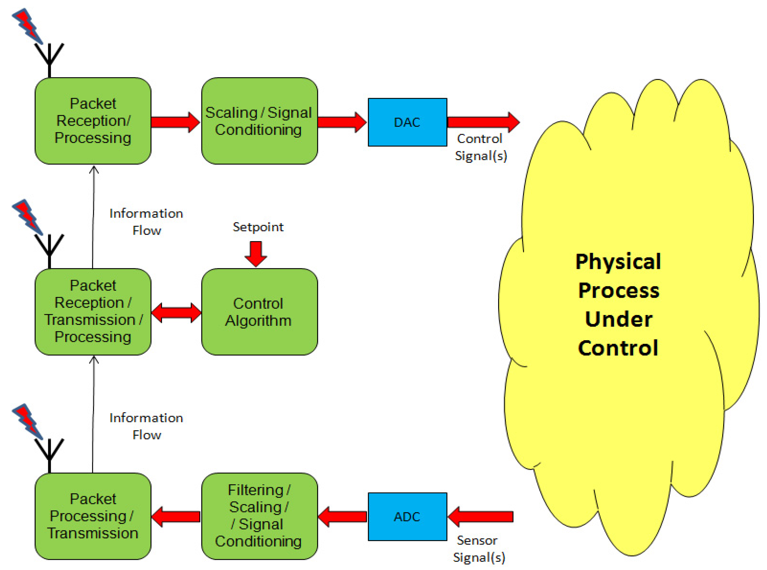
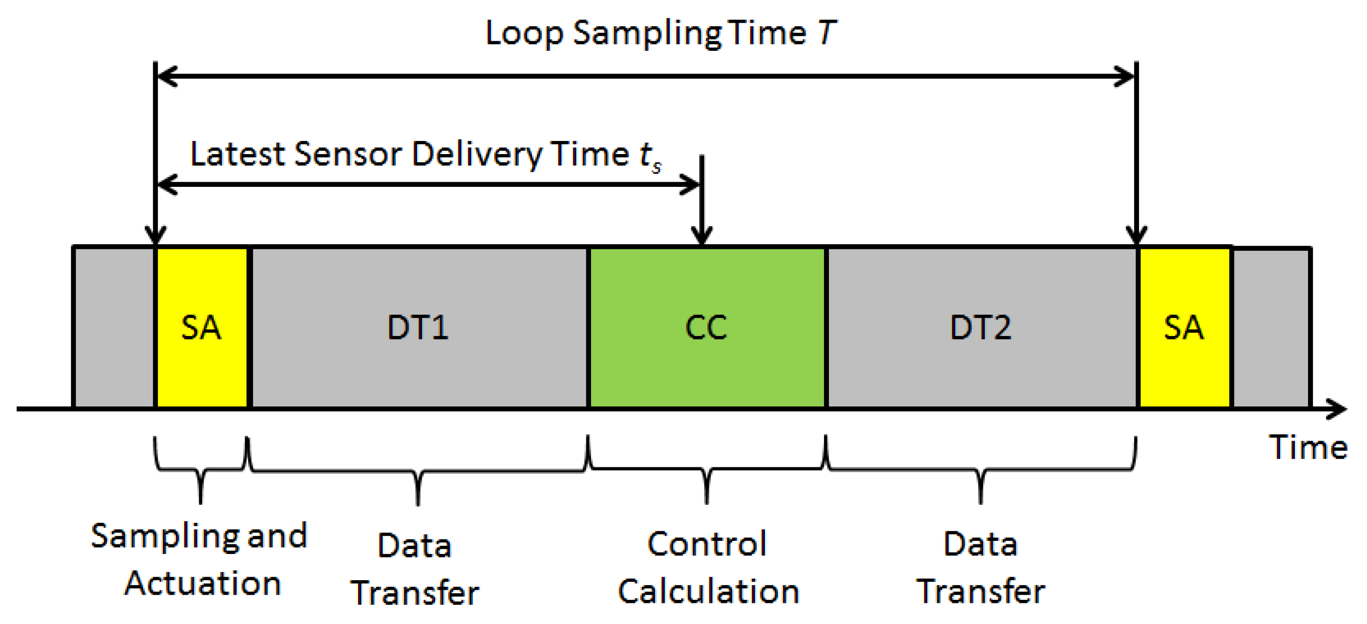
3. General Configuration and Assumptions

Although it is assumed that multiple control loops may be coordinated and scheduled using the technique to be described, for ease of exposition only a single control loop is considered (as depicted in Figure 1). In order to incorporate the possibility of packet re-transmissions or other interference-aware MAC strategies during a transmission round, we also make the simplifying assumption that the sampling and actuation tasks (on the sensor and actuator nodes respectively) take place approximately synchronously, within the level of the global clock accuracy as shown in Figure 2. These synchronized sampling/actuation (SA) events repeat every T time units, where T is the loop sampling time. In between these events, data must first be transferred between the sensor and controller node (data transfer DT1) to enable the control calculation (CC) by the latter. Following the control calculation, data must then be transferred between the controller and actuator node (data transfer DT2) to enable the plant control signal to be updated at the next SA event. Such a structure seems particularly suited to many types of industrial wireless networks, including networks using basic or enhanced TDMA variants [8,10,11,21] and simple master-slave polling [9]. It is also suitable for non-specialized architectures such as WiFi employing sNTP (simple Network Time Protocol) for node clock synchronization.
Figure 2. Loop Timing with Approximately Synchronized Sampling/Actuation.
Electronics 04 00857 g002
Although the assumption of synchronized sampling and actuation introduces an overall extra delay of one sample period T into the control system, it is an effective and commonly used means to limit jitter [15]. In practice, the extra delay is easily dealt with (if the sample time is appropriately chosen) alongside the phase-shift of the Zero-Order-Hold (DAC) by adding an extra time delay of θ = 1.5 T into the delay of the open-loop plant before controller design [15]. Let the kth packet from the sensor node to the controller node contain the sampled-data representation of the process measured variable y(k) obtained from the ADC. Let the kth packet from the controller node to the actuator node contain the sampled data control signal u(k) to be applied to the process manipulated variable via the DAC. Let the worst-case duration of a burst be denoted by the parameter β∈ℵ+, representing the number of sample periods (of length T) that a link may be unavailable. The length of βT may be determined to given confidence limits using statistical data. It is assumed that the maximum burst duration time βT does not allow the clocks to drift beyond their stated tolerance. The final assumption made is that only limited re-transmissions of a process packet are attempted, such that packets are “dropped” by the network if they cannot be delivered before their (firm) deadline.

4. Sensor Packet Loss Compensation

4.1. Principle

Considering Figure 1, the first source of potential information losses in the control loop lies in the wireless link between the sensor and controller nodes. Under the assumption that a large proportion of samples will be successfully delivered in a well-designed wireless network, one possible way to add resilience against such information losses in the loop is to use buffering. Since the control loop is real-time, only known information at sample index k can be transmitted by the sensor node at this time instant; therefore, the measured process output at sample k + 1 cannot be transmitted. Nevertheless, a prediction of its value could still be formed in the controller node. The adaptive compensator proposed in this paper therefore consists of three main elements which mainly reside inside the controller node. Suppose that the sensor-controller data packet transfer (DT1 in Figure 2) has an effective deadline of ts time units, where ts < T. This effective deadline is such that if the controller node does not begin the process of control calculation and initiation of data transfer DT2 in Figure 2, the actuator node does not have a chance of receiving the data before the next actuation event. A packet omission for the kth iteration of the loop can easily be detected in the controller node by the absence of a new packet at time kT + ts. The schedule decoder/packet loss detector is responsible for providing the indication of successful/ unsuccessful packet receipt to a switching mechanism. In the case of a successful receipt, y(k) may be retrieved from the packet and forwarded to the control module. In the case of unsuccessful receipt, the switching mechanism instead forwards an estimate of the omitted packet’s content ŷ(k) to the controller. This estimate is produced by an adaptive process model. The model continually uses a technique—to be described below—to predict the values of missing samples, by monitoring the time history of the control signal u(k) and the actual/estimated process values y(k) and ŷ(k) respectively. When packets arrive successfully, the actual process output is employed to apply corrections to the process model parameters, to ensure it remains “up to date”. Information loss is further minimized by buffering and transmitting multiple samples in the sensor node, such that at sample index k, measured values for y(k), y(k − 1), y(k − 2), … , y(kH) are always transmitted for some horizon length H. Under the assumption that the horizon H ≥ β, good resilience to burst errors is achievable since any information lost during a burst can be recovered upon the arrival of the first packet. Since a DCS sensor sample is often encoded as a 16-bit integer, the overhead of such an approach is typically only 2H extra bytes per packet which is relatively small.

4.2. CARIMA Process Model

In the design of a sampled-data control system, a nominal model of the process to be controlled will normally be identified by the control engineers at an early stage of the design process. An Auto Regressive Moving Average (ARMA) model is often used for this. However, for predictive purposes, the ARMA model does not include the effects of potential disturbances and can perform poorly in practical situations; in addition, the model parameters may not be accurately known or may “drift” with time. To overcome the first of these problems, a Controlled Auto-Regressive Integrated Moving Average (CARIMA) model can instead be adopted:
A ( z 1 ) y ( k ) = z d B ( z 1 ) u ( k ) + ν ( k ) Δ
Where z1 is the backward shift (delay) operator, y(k) and u(k) represent the process output and input at sample index k, ν(k) is a zero-mean white sequence and the difference operator Δ = 1 − z−1. A and B are both polynomials in z1 having the following definitions:
A ( z 1 ) = 1 + a 1 z 1 + a n z n B ( z 1 ) = b 0 + b 1 z 1 + b m z m
In the model represented by Equation (1), d represents the integer part of the system time-delay such that b0 is non-zero and, assuming that a zero order hold (DAC) is employed for control purposes, will always satisfy d ≥ 1 (if the synchronized sampling/actuation strategy as depicted in Figure 2 is also employed, it follows that d ≥ 2). The transfer function model described by Equations (1) and (2) is representative of many types of real-world physical processes, see for example [27,28], and is employed for advanced control techniques such as the Generalized Predictive Control (GPC) method [28]. The integrated white noise sequence in the model corresponds to unknown disturbance terms entering the system input, and stochastic behavior (random steps at random times) is well captured. Note that all disturbances (e.g., those on an output) can be referenced to a system’s input via a simple transformation [27]. In terms of creating accurate short-term predictions of the process output, after multiplying out the delta term in the model given by Equation (1), it may be solved for Δy and transformed into an appropriate difference Equation:
Δ y ^ ( k ) = a 1 Δ y ( k 1 ) a n Δ y ( k n ) + b 0 Δ u ( k d ) + + b m Δ u ( k d m ) + υ ( k )

4.3. Packet Loss Compensation

Assuming that the time history of the process input and output is known at sample instant k, then as E{ν(k + j)} = 0 ∀ j > 0, i.e., the expected future values of the unknown disturbance sequence are zero, Equation (3) may be used to predict the expected change in the process output at sample k + 1. Recursion upon this equation can then be used to obtain the change in the output at steps k + 2, k + 3, … assuming that Δu(k + 1), Δu(k + 2), … , and so on are known. Assuming that the last successful packet reception was at sample interval k, and j consecutive samples have since been lost, Equation (4) below allows the prediction of the k + jth process output:
y ^ ( k + j ) = y ( k ) + i = 0 j Δ y ( k + i )
Thus upon omission of a packet, the value of the lost process information may be reconstructed using Equation (4) with complexity dependent upon the number of terms in the model. With this prediction the controller is effectively calculating the required open-loop control to drive the process towards the current reference, with disturbances entering the system at or before the time that the last packet was successfully received being taken into account. Assuming that the model is of reasonable quality and the burst duration β is not excessive, the compensator will achieve a reasonable quality of control. In most real situations the coefficients of the model represented by Equation (1) may not be accurately known, they may only be partially known, or they may in fact be time-varying due to inherent process non-linearity and wear and tear of components. This warrants the use of an on-line parameter identification technique for their identification, to be described below.

4.4. Adaptive Parameter Updating

Under the assumption that a high proportion (≈99.9%) of samples will be successfully delivered in a well-designed wireless network [3,8,9,12], statistically there is a large amount of process information available which can be used to recursively update the process model parameters. In order to adaptively track parameter variations, the Recursive Least Squares (RLS) algorithm may be employed [27]. Firstly, the CARIMA model parameters at sample instant k may be written in vector form:
θ ( k ) = ( a 1 ( k ) , a 2 ( k ) , , a n ( k ) ,    b 0 ( k ) , b 1 ( k ) , , b m ( k ) )
And the vector of independent variables x(k) which is constructed from the previous input/output process data can be written as:
x ( k ) = ( Δ y ( k 1 ) , , Δ y ( k n ) , Δ u ( k d ) , , Δ u ( k d m ) )
In both cases, the length of the vectors is equal to m + n. Equation (3) may then be rewritten in a form suitable for on-line estimation as:
Δ y ^ ( k ) = θ T ( k ) x ( k )
When a packet is successfully delivered at sample index k, the parameter vector can be updated based upon the prior error ep(k) between the predicted and actual change in process values. Using the parameter vector from step k − 1 yields:
e p ( k ) = Δ y ( k ) ( θ T ( k 1 ) x ( k ) )
Defining the update rule for the inverse of an (m + n)-by-(m + n) symmetric “information matrix” P as follows:
P ( k ) 1 = λ P ( k 1 ) 1 + x ( k ) x ( k ) T
where λ ∈ (0,1] is a “forgetting factor” which is used to exponentially reduce the weight or importance of past data by a factor λ at each step. The choice of λ can impact upon the speed of adaptation and also the stability of the estimator; values close to unity lead to slower convergence with increased stability, while smaller values lead to faster tracking with reduced stability. The asymptotic memory length N (in samples) of the RLS estimator with non-unity forgetting factor λ is given by N = 1/(1 − λ). The memory length is effectively a time-constant indicating the rate at which information is lost, which provides some guidance on an appropriate choice for λ [28]. For most process control applications, in the absence of any knowledge on the rate of parameter fluctuations previous work suggests to use a memory length between ≈ 1000 to 10,000 samples, i.e., to use λ ∈ [0.995, 0.9999] [27,28]. If no parameter fluctuations are expected then information loss can be disabled by setting λ = 1. In some situations it may be prudent to employ a variable forgetting factor λ(k) to prevent co-variance wind-up when the input signal is expected to be stationary for long intervals (e.g., with the process in steady-state)—further details can be found in [27] and [28], and the references contained therein. After computing Equations (8) and (9) at sample k, the parameter vector can then be updated using the main RLS computation which is as follows:
θ ( k ) = P ( k ) x ( k ) e p ( k )
To remove the need for direct matrix inversion, the Sherman-Morrison formula may be used to directly update P with P(0) initialized to a suitable value, e.g., I × 10−6. The implementation complexity of such a procedure is O((m + n)2) per iteration due to the need to provide the rank-1 correction to matrix P before application of (10) [27]. Although this is reasonably small, in order to keep the overheads of the scheme to a minimum, the model order should ideally be kept to a small value. In the next Section it is argued that under the previous assumptions of the paper, (m + n) ≤ 10 holds for many of the systems of interest in this paper.

4.5. Practical Industrial Process Model

Although there is a near-infinite amount of possible configurations of industrial process plant, it is well known that a large majority may be described (for small perturbations around an operating point) by low-order transfer function models incorporating time delays [27,29]. In addition, well-known estimates have suggested that over 90% of industrial control system implementations worldwide are of the Proportional Integral Derivative (PID)-type; the algorithm is the standard tool for industrial automation [27]. A representative model commonly employed for PID control designs is the “Second Order Plus Dead-Time” (SOPDT) Model represented by Equation (11):
G ( s ) = K ω n 2 e s θ s 2 + 2 ζ ω n s + ω n 2
This model requires only four parameters, namely the static gain K, natural frequency ωn, damping ratio ζ and time delay θ. Assuming the sample time does not exactly divide the delay, digitization of (11) results in the CARIMA model represented by Equation (12):
( 1 + a 1 z 1 + a 2 z 2 ) y ( k ) = z d ( b 0 + b 1 z 1 + b 2 z 2 ) u ( k ) + υ ( k ) Δ   
where d = ⌊θ/ts⌋ and the A and B parameters can be obtained via the Z-transform. Note that the assumption of fractional delay also allows the possibility of the model given by Equation (11) including a (possibly non-minimum phase) zero. In situations where θ (and hence d and B) may also be time-varying, then the 3-term B polynomial in (12) may be expanded to cover all possible values of delay within a specified bound. A drawback in this situation is the potentially large number of additional parameters that require identification by RLS [27]. Under the assumption that PID control is applied to the process and the sample rate is selected to be approximately equal to one sixth of the 10%–90% open-loop rise time of the process [15,29], then an upper bound of 8 parameters for B may be determined. This follows because PID control is seriously degraded by systems having a time delay larger than approximately twice the dominant time constant of the process. If the delay is larger than this, then the degradation of employing PID control will be commensurate (or worse) with that of experiencing long burst errors. Including the two parameters required for the process poles a1 and a2 gives a total of 10 parameters to cover a large majority of industrial processes under PID control. In order to prevent covariance wind-up when insufficient excitation is present in input signals during recursive estimation (as detailed above), a simple conditional updating scheme with low CPU overhead can be employed as an alternative to a variable forgetting factor. In this scheme, when λ < 1 is employed the parameter updates occur only when the inequality xT(k) P(k) x(k) > 2(1 − λ) is satisfied: satisfaction of this condition ensures that the input vector is sufficiently exciting [27].

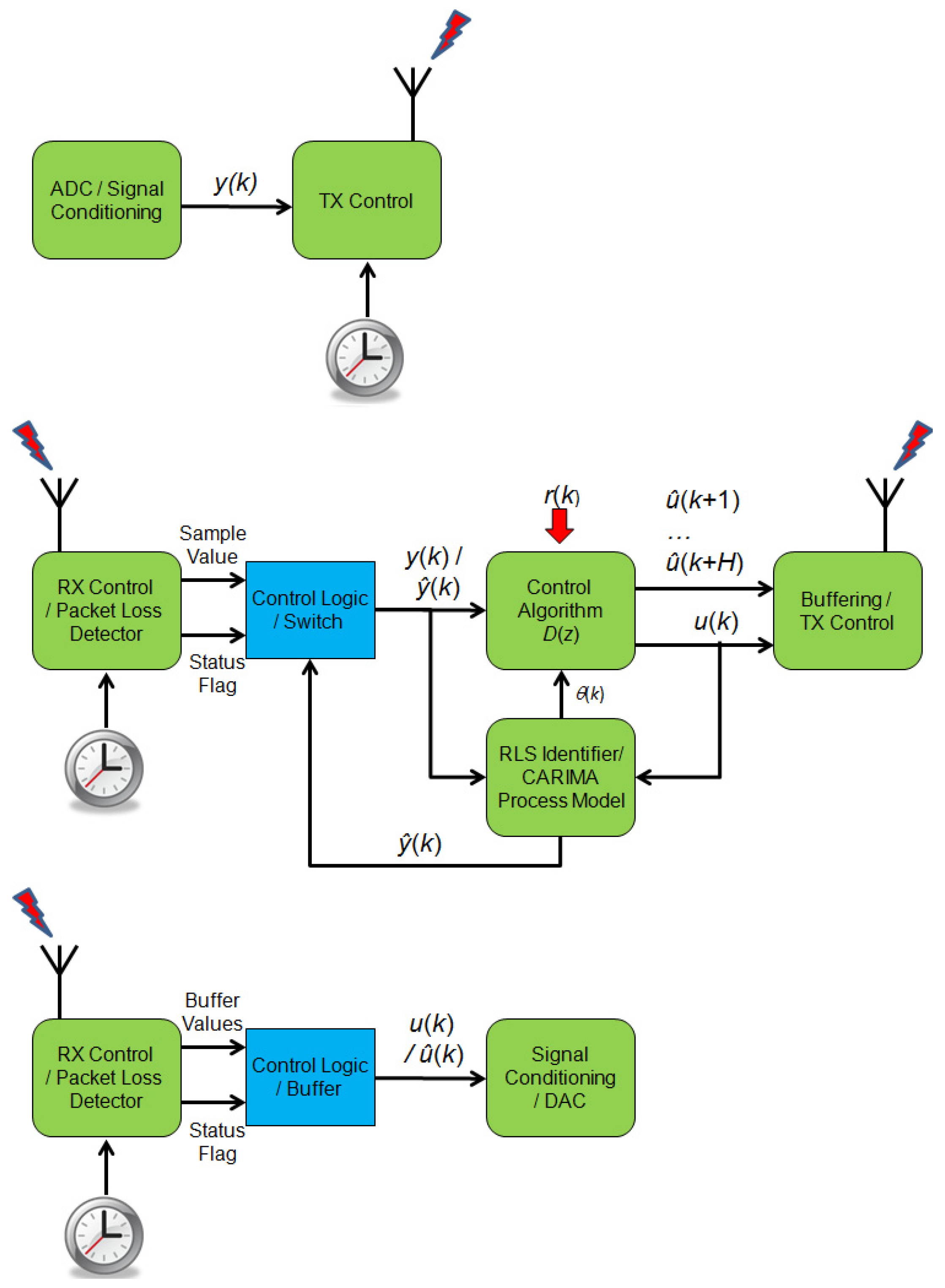
5. Controller Packet Loss Compensation

5.1. Principle

Considering Figure 1, the other source of potential information losses in the control loop lies in the wireless link between the controller and actuator nodes. Again, under the assumption that a large proportion of samples will be successfully delivered in a well-designed wireless network, one possible way to add resilience against such information losses in the loop is to use buffering. Suppose that the controller is implemented as the causal, discrete control law D(z) = U(z)/E(z), where U(z) and E(z) are the z-transformed representations of the sampled-data control signal u(k) and feedback error e(k) = r(k) − y(k), with r(k) the reference (setpoint) signal at step k. Then upon receipt of the new actual/estimated process value y(k) or ŷ(k), the controller will first form the new error e(k) and then the new control signal u(k) via D(z).
Since the control u(k) (and hence Δu(k)) are available, the prediction equation (3) allows the calculation of ŷ(k + 1). Under the assumption that r(k + 1) = r(k), ê(k + 1) can also be calculated and hence û(k + 1|k) determined through the control law D(z). This procedure may be applied recursively to determine the future controls to apply over a horizon of H samples, i.e., the signals u(k), û(k + 1|k), û(k + 2|k), … , û(k + H|k). This sequence effectively represents the “best guess” of future open-loop controls that would be generated by controller D(z) to drive the process Model (1) towards the current reference r(k), and can be calculated with a complexity dependent upon the number of terms in the model and controller, and the length of H. It is the “best guess” in the sense that disturbances entering the system at or before the time that the last sensor packet was successfully delivered are taken into account, but those affecting the system after this time are not. Since the process model parameters are accurately tracked by RLS, and assuming the controller D(z) achieves the desired closed-loop performance, then this sequence of open-loop controls should achieve a reasonable quality of control. In the buffering approach, at each sample time the controller node re-calculates this sequence and places it in the packet to be forwarded to the actuator.
The controller-sensor data packet transfer (DT2 in Figure 2) has an effective deadline of T time units after the start of the previous actuation event. A packet omission for the kth iteration of the control loop can easily be detected in the actuator node by the absence of a new packet at time t = kT. In this case, supposing that packet k − 1 arrived successfully, the estimated control û(k|k − 1) can be applied instead of u(k). In the case of multiple successive controller-actuator packet omissions, then if the last successful packet was received at step j (with j < kj + H), there is an estimated control û(k|j) available to apply to the process. Under the assumption that the horizon H ≥ β, good resilience to burst errors is achievable. Since a DCS control signal is often encoded as a 16-bit integer, the overhead of such an approach is typically only 2H extra bytes per packet which is relatively small.

5.2. Adaptive Digital PID-Like Control Law

As mentioned, with knowledge of the process parameters, a control law for the identified plant model can be designed. It has been estimated that over 90% of industrial control system implementations worldwide are of the PID-type; in this section, practical details of the application of the buffering method to a simple anti-wind-up digital PID-like controller will be discussed. Consider a digital controller for the plant (1), and assume that A(1) ≈ 0. Assume that the closed-loop is required to have dynamics given by:
G C L ( z ) = D ( z ) G ( z ) 1 + D ( z ) G ( z ) = z d K p B ( z ) P ( z )
where Kp = P(1)/B(1) to ensure offset-free control and P(z) is a stable monic polynomial which forms the design specification, and is typically of first or second order. Observe that the numerator in (13) is a scaled version of the process open-loop numerator; as such there is no cancellation of open loop zeros and the closed loop effectively contains the same delay as the open loop process. Solving expression (13) for the required controller D(z):
D ( z ) G ( z ) 1 + D ( z ) G ( z ) = z d K p B ( z ) P ( z ) P ( z ) D ( z ) G ( z ) = z d K p B ( z ) ( 1 + D ( z ) G ( z ) ) = z d K p B ( z ) + z d K p B ( z ) D ( z ) G ( z ) P ( z ) D ( z ) G ( z ) z d K p B ( z ) D ( z ) G ( z ) = z d K p B ( z ) D ( z ) ( P ( z ) G ( z ) z d K p B ( z ) G ( z ) ) = z d K p B ( z ) D ( z ) = z d K p B ( z ) P ( z ) G ( z ) z d K p B ( z ) G ( z ) = z d K p B ( z ) P ( z ) z d B ( z ) A ( z ) z d K p B ( z ) z d B ( z ) A ( z ) D ( z ) = z d K p B ( z ) A ( z ) P ( z ) z d B ( z ) z d K p B ( z ) z d B ( z ) = K p A ( z ) P ( z ) z d K p B ( z )
Given the choice of Kp, one sees that the controller (14) contains an integrator since P(1) − Kp B(1) = 0. In the adaptive design procedure, both A(z) and B(z) are estimated directly by RLS as described in Section 4.4 and P(z) is specified by the designer; hence the controller is trivial to implement as the control gains are very simple functions of the estimated plant parameters and design specification. A typical design specification is to set P(z) = 1 − p1z−1, i.e., a first-order exponential response with parameter p1. When this first-order specification is used with the simple plant Model (12), the classical adaptive controller of Vogel and Edgar [30] is recovered. In the controller (14), however, one may actually use any plant model G(z) and any suitable monic polynomial P(z). Hence the proposed controller design given by (14) is a generalized form of this adaptive controller. The described approach is an identifier-based Certainty-Equivalence pole-placement design, in which minimum-variance parameter estimates are obtained by RLS and a deterministic Linear Time Invariant (LTI) compensator is designed based upon these estimates [27]. The derivation leading to expression (14) given above ensures that D(z) gives closed-loop poles located at P(z). To implement anti-wind up for this controller, assuming that the process actuator has upper and lower amplitude and rate saturation limits denoted as umax, umin, Δumax and Δumin respectively, then the anti-wind-up control law can be implemented as:
Δ u ( k ) = s a t { u ( k ) u ( k 1 ) , u , u + } u ( k ) = u ( k 1 ) + Δ u ( k )
where the unconstrained u(k) is first computed, sat{} is the usual saturation function and the saturation limits u+ and u are taken as:
u + = min { u max u ( k 1 ) , Δ u max } u = max { u min u ( k 1 ) , Δ u min }

5.3. Integrating Processes

Integrating processes are sometimes found in process control and servo applications. In order to deal with systems with an open-loop integrator, a slight modification to the above method is needed as the cancellation of the process poles with the controller zeros as described in the steps above may be ill-conditioned and result in controllability issues. When an integrator is present in the process, A(z) may be factored as (1−z−1) A’(z) and the use of the controller given by Equation (14) results in a common factor of (1−z−1) in both the controller numerator and denominator in the steady-state (i.e., as z tends to 1). Firstly, observe that the following condition can be easily checked to detect the presence of one or more integrators:
| A ( 1 ) | = | 1 + i = 1 n a i | ε
where ε is a suitably small constant e.g., the machine epsilon of the implementation processor. When this condition holds - and assuming that only one integrator is present in the plant - we wish to instead design a PD-like controller. This can be achieved by cancelling the common factor (1 − z−1) in the controller (14), which is a straightforward procedure [27].
The incremental version of this PID-like algorithm implementation as given by Equation (15) seems particularly well suited to the proposed compensation method, since one may first calculate Δu(k) and u(k) from Equations (15) and (16), and since e(k) = r(k) − y(k), Δê(k + 1|k) = −Δŷ(k + 1|k) the latter of which is obtained from Equation (3). This leads on to the straightforward calculation of Δû(k + 1|k) and Δê(k + 2|k) and so on, allowing the buffer to be filled with the required projected controls with relative ease. The structure of the proposed system is as shown in Figure 3. The overhead of implementing the proposed adaptive control law is linear in the size of the estimated plant parameter vector, with overall complexity O(n + m). A structural overview of the elements of the proposed system is as shown in Figure 3.
Figure 3. End-to-end elements of the proposed compensation technique (top: sensor node, middle: controller node, bottom: actuator node).
Electronics 04 00857 g003

6. Computational Study
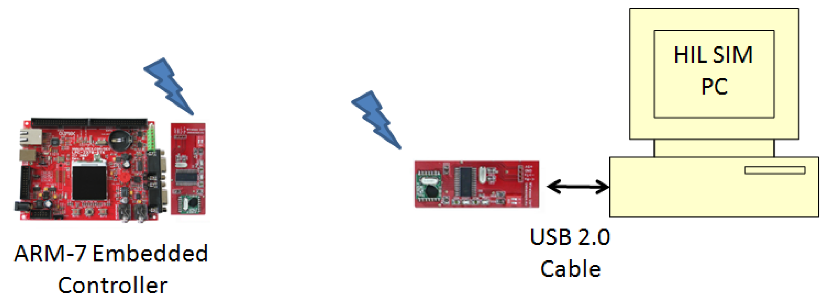
6.1. Test Facility

A prototype DCS employing a wireless network was constructed to test the principles discussed in previous Sections. In the test bed, the overall structure of which is as shown in Figure 4, a real-time Hardware-In-The-Loop (HIL) approach was used in order to be able to evaluate control performance and CPU overheads for the method applied to a typical process plant. The Simulink© Real-Time Windows Target (RTWT) environment was employed to run a real-time simulation of a process model on the HIL simulation PC. Given the simplicity of the implementation details of the sensor and actuator nodes, their operations were integrated into the simulation model employed by the HIL simulation PC. The real-time controller node consists of an embedded processor employed to implement the functionality of the central control node. The main processing element in the node hardware platform is a 32-bit LPC2387 microcontroller with ARM7TDMI-S core from NXP semiconductors, mounted on a development board manufactured by Olimex©. The device was operated with a CPU clock speed of 72 MHz, and it features 512 Kb of on-chip flash, 98 Kb of on-chip RAM plus a rich set of I/O peripherals including multiple UARTs. In order to implement the wireless communication link, a set of simple RF serial communication transceivers from USBscope© were employed. These devices work at 433 MHz, have a range of approximately 400 m and implement half-duplex RS-232/485-like links at each end, operating at 57,600 bps. A transceiver was interfaced directly to an on-chip UART of the LPC2378 to implement RF communications with a similar transceiver interfaced to the simulation PC via USB.
Figure 4. Prototype test facility.
Electronics 04 00857 g004
In this study, 24-byte packets were used: two bytes for addressing, a 20 byte payload, plus a two byte checksum. This allows for up to 10 control signals of resolution 16-bits each to be transmitted per packet. Serial port emulation was employed on the HIL simulation PC, to enable data to be exchanged with RTWT via packet input/output blocks. Packet I/O is well supported in the RTWT environment, with “error” and “data ready” signals being available in order to control the buffering scheme in the simulated actuator node and controller nodes. This setup had the added advantage that sensor and/or controller packet losses may also be enforced using fault injection within the Simulink model, which can be driven by representative stochastic models (e.g., [13]). The techniques proposed in the previous Sections were coded into a small embedded “C” library for test purposes, and the routines were embedded onto the controller node and linked into RTWT function blocks as appropriate.

6.2. Experimental Design

In our previous work [14], experiments have been described that demonstrate promising behavior of the proposed packet loss compensator. When used with a simple PD controller, performance was shown to be superior to that a simple derivative disabling technique with only a very modest increase in overheads. In this paper, the proposed compensator is investigated in more depth and is employed in conjunction with both the control buffering technique and controller design as proposed in Section 5. In these experiments, overhead and performance comparisons were made to the packet buffering and robust compensator as described in [23]. In this technique, once the plant parameters have been identified controller zeros are employed to cancel the process open-loop poles and integral action is used in the controller. The loop gain is selected to ensure a specific phase margin is achieved by carrying out a frequency sweep of the combined process, controller and buffer-induced delays to determine the critical gain. The frequency test interval is bounded by DC and the Nyquist frequency, and is divided into a grid of S test points; the larger the value of S the better the accuracy of the method but the higher the computational overhead as O(S × (m + n)) FLOPS are required along with numerous trigonometric and square root operations (although the former can be pre-computed at each frequency test point and stored in a table).
For reasons discussed in [14] and elsewhere, systems with faster dynamics will be more susceptible to burst errors lasting a given temporal duration. In this case study, a servomotor was chosen as the process to control; this is a common choice for evaluating DCS performance [24]. The continuous-time dynamics relating the shaft speed to the armature voltage of the servomotor can be described by the transfer function:
G ( s ) = 2 1 + 0.5 s
In order to add further realism into the simulation, quantization corresponding to a 16-bit shaft encoder was employed, plus a small amount of zero-mean measurement noise (equivalent to ± 1 encoder bit) was injected into the output of the simulation model. Note that although the nominal model given by Equation (18) was known in this case, the adaptive compensator and controller were “cold-started” with no prior knowledge of process parameters included. A fixed forgetting factor λ = 1 was employed by the identifier as no process parameter variations were expected. Identical noise sequences were employed in each of the described experiments that follow. The main objective of the experiments was to determine the ability of both schemes to compensate for the effects of burst errors. In order to numerically quantify this ability, the experiments were designed as follows. Firstly, the Robust Control (RC) scheme was applied to control the nominal model given by Equation (18) with a target phase margin pm = 60° selected, grid size S = 100 and sampling time T = 0.1 s employed. For reasons that will shortly be described, the sensor-controller and controller actuator buffers were set to a size of 10 samples each. The resulting closed-loop response was found to be well approximated by the following second order transfer function:
G ( s ) = 0.35 e s s 2 + 0.8 s + 0.35
Next, the proposed Predictive Control (PC) method was employed using the same sample time of T = 0.1 s, with a design polynomial P(z) = 1 − 1.9198 z−1 + 0.9231 z−2, i.e., the discrete equivalent of the denominator of the transfer function given by Equation (19) using a sample time of 0.1 s. This gave approximately the same nominal closed-loop behavior between the two methods (save for the additional 1 second delay in the RC design). At this stage, two experiments were then carried out. In both cases, the control system was required to track an input sinusoidal reference with amplitude 10 and period 20 s for 3,600 s. The Integral of Squared Error (ISE) between the process output and the closed-loop reference model (19) was measured in both cases, giving a measure of the nominal (error free) performance of the control loops. Following this, the experiments were repeated under fault injection. In order to simulate the effects of burst errors, simple Markov model (see [20] for details) was employed to inject burst errors on the HIL PC links (in both sensor-controller and controller-actuator links) at an accelerated rate, with mean burst inter-arrival of 5 s and mean burst duration of 0.4 s. For the RC design, a buffer size of 10 samples in each link was employed ensuring that ≈ 95% of burst lengths would be covered by the buffer. For the proposed compensator, the same buffer size of H = 10 samples was used with a sensor node packet deadline of ts = 0.05 s employed in the controller node. The experiments were again executed for 3600 s, with the ISE measured in both cases and with identical patterns of burst errors employed. The ratio of the ISE value obtained under error conditions to the nominal ISE value therefore gives a measure of the ability of the method to tolerate the errors, with a larger value indicating worse closed-loop performance. During the course of the experiments, CPU execution times on the embedded controller node were recorded using an on-chip timer with 0.1 μ second resolution.

6.3. Experimental Results

Table 1 shows the ISE results and CPU execution times (in milliseconds) that were obtained over the course of the experiments; the ISE increase between nominal and error case is quoted as a percentage. Note that in the execution times, only the time required to design and apply the controller is reported; an additional 1.486 ms execution time was required for plant identification in both methods, and is not added to these figures. Figure 5 shows a snapshot of the comparative performance of behaviors for the two methods for the first 100 s of each experiment; the upper section of the figure shows the process outputs whilst the lower sections are indicators of burst errors, the lines having a value of 1 when a packet loss occurs and 0 otherwise. Please note that in both cases, the controller was disabled for the first 10 s to allow initial parameter convergence and a pulse input was applied to the process. This is a typical strategy for an adaptive controller to help prevent large initial swings in the control input and aid model identification. The upper section of this indicator represents losses in the sensor-controller link, while the lower represents losses in the controller-actuator link. As may be observed, the closed loop responses are very similar (with the RC method having an additional 1 second delay), and all bursts are well-tolerated during this initial period. The evolution of the estimated process parameters for the PC method is shown in Figure 6 (the estimated parameters for the RC method follows an almost identical trajectory). Digitizing the transfer function given by Equation (18) with a sampling time of T = 0.1 s yields the discrete equivalent transfer function shown in Equation (19), where an extra one-sample delay has been added due to the synchronized sampling-actuation in the control workflow (Figure 2). The two dominant identified parameters (b2 and a1) are shown bolded in the Figure (note that due to the identification mechanism, the “a” parameters have reversed signs); the remaining parameters have values in the range [−0.01, 0.01] and most are close to zero. Such residual effects are common in the presence of noise when using an over-parameterized B polynomial. Comparing the parameter values observable in Figure 6 with the parameters in the model given by Equation (19), one sees a stable and rapid convergence to appropriate values for the two key parameters.
G ( z ) = 0.3625 z 2 1 0.8187 z 1
Table 1. Comparative evaluation of Integral of Squared Error (ISE) ratios and CPU Execution Times.
MethodISE Ratio (%)Exec Time (ms)
RC Method677.02461.345
PC Method319.0870.268
Figure 5. (A) effects of burst errors with RC (solid) vs. PC Method (dashed); (B): sensor-controller node link state; (C): controller-actuator node link state.
Electronics 04 00857 g005
Applying the design formulate represented by Equation (14) using the model given by Equation (19) as the process G(z) gives an ideal controller design D(z) to be employed in the PC method given as Equation (20). Examining Figure 5, one can see that allowing for the impact of packet losses, the reference is tracked very well, and the effective controller designed on-line by the PC method implementation (using the parameters identified in as shown in Figure 6) gives a controller very close to the ideal. The residual effects of noise on the parameter identification have had little impact, as expected [28].
G ( z ) = 0.009 ( 1 0.8187 z 1 ) 1 1.9198 z 1 + 0.9198 z 2
Figure 6. Evolution of identified process parameters for the model used in the experiments. The two dominant parameters (b2 and a1) are shown bolded.
Electronics 04 00857 g006
From these data and recorded responses, it can be observed that both methods experienced a deterioration of performance during the course of the experiments. This deterioration is to be expected, since both methods rely on buffering schemes in the path from controller to actuator and identical buffer sizes were employed. The selected buffer size of 10 samples in each case covers around 95% of the injected bursts, but several bursts of longer duration were generated. In these situations, a loss of information inevitably occurs. However, the PC method—with a smaller ratio of ISE increase—was better able to maintain the nominal loop performance than the RC method. The difference in these deterioration ratios is a factor of over 2. Since the controllers were tuned for almost identical nominal loop performance, it would seem that this reduced susceptibility seems due to the actions of the predictive packet loss compensator in the path between the sensor and actuator. Even in situations in which durst durations exceed 10 samples—causing information loss in the RC scheme—the model of the PC continues to serve an output predicted from the last good sample, allowing appropriate open-loop controls to be applied. Comparing the obtained execution times, one may observe that the CPU overhead from implementing and designing the predictive controllers is significantly different between the methods, with the RC scheme taking nearly 229 times longer to design and apply the controls. This is not surprising as the method required the solution of a difficult non-linear search problem. The computation time can of course be reduced with a corresponding reduction in S, but this leads to further performance degradation (in fact, the method fails completely with S < 30 as insufficient points are then employed to parameterize the frequency response and correctly achieve the phase margin). In summary, the proposed controller design technique seems to be a simple and low-overhead means to design a digital PID-like controller for use with the proposed adaptive/predictive packet loss compensator. This compensator has good resilience to packet losses between the sensor-controller. The suggested packet buffering scheme employed in the controller-actuator link seems to be a weaker link, but still performs as well as a regular playback buffer without inducing delays in the link. However performance deterioration can still occur in situations in which a burst length exceeds the buffer size. The use of more reliable compensation methods in this link will be a focus of our future work.

7. Conclusions and Further Work

This paper has considered an adaptive/predictive compensation scheme to help ameliorate the effects of packet losses in industrial DCSs employing wireless control loops. Experimental results have been reported that illustrate that for a small increase in packet processing and controller overheads, the method has the potential to improve upon contemporary schemes designed for use with industrial PID and PID-like controllers, even in cases when no specific knowledge of the process parameters are available. The proposed methods give robustness to packet losses around the control loop and exhibits bounded and relatively low computational complexity; as the majority of the overhead resides in the central controller node, they seem well suited for industrial DCS systems. Future work will concentrate upon further testing of the scheme using both HIL simulation and practical field testing.

Author Contributions

Michael Short developed the initial ideas for the compensators contained within this article, the control design method, and created the manuscript draft. Usama Abrar progressed the sensor loss compensator to a prototype testing stage. All three authors contributed to the final system prototyping and experimental evaluation/analysis, and proof-reading of the manuscript.

Conflicts of Interest

The authors declare no conflict of interest.

References

  1. Flammini, A.; Ferrari, P.; Marioli, D.; Sissini, E.; Taroni, A. Wired and wireless sensor networks for industrial applications. Microelectron. J. 2009, 40, 1322–1336. [Google Scholar] [CrossRef]
  2. Thompson, H.A. Wireless and Internet communications technologies for monitoring and control. Control Eng. Pract. 2004, 12, 781–791. [Google Scholar] [CrossRef]
  3. Munir, S.; Lin, S.; Hoque, E.; Nirjon, S.M.S.; Stankovic, J.A.; Whitehouse, K. Addressing burstiness for reliable communication and latency bound generation in wireless sensor networks. In Proceedings of the 9th ACM/IEEE International Conference on Information Processing in Sensor Networks (IPSN), Stockholm, Sweden, 12–15 April 2010; pp. 303–314.
  4. Ikram, W.; Thornhill, N.F. Wireless communication in process automation: A survey of opportunities, requirements, concerns and challenges. In Proceedings of the 8th UK Automatic Control Conference (UKACC), Coventry, UK, 7–10 September 2010.
  5. Oliver, R.S.; Fohler, G. Timeliness in wireless sensor networks: Common misconceptions. In Proceedings of the 9th International Workshop on Real-Time Networks (RTN), Brussels, Belgium, 6 July 2010.
  6. Ghostine, R.; Thiriet, J.M.; Aubry, J.F. Variable delays and message losses: Influence on the reliability of a control loop. Reliab. Eng. Syst. Saf. 2011, 96, 160–171. [Google Scholar] [CrossRef]
  7. Rothmensen, S. The reality of wireless real-time: Wireless networks in industrial automation. In Proceedings of the Keynote Speech at the 9th International Workshop on Real-Time Networks (RTN), Brussels, Belgium, 6 July 2010.
  8. Suriyachai, P.; Brown, J.; Roedig, U. Time-critical data delivery in wireless sensor networks. In Proceedings of the International Conference on Distributed Computing in Sensor Systems (DCOSS10), Santa Barbara, CA, USA, 21–23 June 2010; pp. 216–229.
  9. Gamba, G.; Tramarin, F.; Willig, A. Retransmission strategies for cyclic polling over wireless channels in the presence of interference. IEEE Trans. Ind. Inform. 2010, 6, 405–415. [Google Scholar] [CrossRef]
  10. Gobriel, S.; Cleric, R.; Mosse, D. Adaptations of TDMA scheduling for wireless sensor networks. In Proceedings of the 7th International Workshop on Real-Time Networks, Prague, Czech Republic, 1 July 2009.
  11. Costa, R.; Portugal, P.; Vasques, F.; Moraes, R. A TDMA-based mechanism for real-time communication in IEEE 802.11e networks. In Proceedings of the 15th IEEE International Conference on Emerging Technologies and Factory Automation, Bilbao, Spain, 14–17 September 2010.
  12. Boggia, G.; Camarda, P.; Grieco, L.A.; Zacheo, G. Toward wireless networked control systems: An experimental study on real-time communications in 802.11 WLANs. In Proceedings of the 2008 IEEE Workshop on Factory Communications Systems, Dresden, Germany, 21–23 May 2008; pp. 149–155.
  13. Jonsson, M.; Kunert, K. Towards reliable wireless industrial communication with real-time guarantees. IEEE Trans. Ind. Inform. 2009, 5, 429–442. [Google Scholar] [CrossRef]
  14. Short, M.; Abrar, U.; Abugchem, F. Application level compensation for burst errors in wireless control networks. In Proceedings of the 17th IEEE International Conference on Emerging Technology & Factory Automation, Krakow, Poland, 17–21 September 2012.
  15. Bennett, S. Real-Time Computer Control: An Introduction; Pearson Education Limited: New York, NY, USA, 1988. [Google Scholar]
  16. Vasyutynskyy, V.; Kabitzsch, K. Event-based control: Overview and generic model. In Proceedings of the 2010 IEEE Workshop on Factory Communications Systems, Nancy, France, 21–23 May 2010; pp. 271–279.
  17. Chen, D.; Nixon, M.; Mok, A. WirelessHART: Real-Time Mesh Network for Industrial Automation; Springer-Verlag: London, UK, 2010. [Google Scholar]
  18. Ferreira, J.; Oliveira, A.; Fonseca, P.; Fonseca, J.A. An experiment to assess bit error rate in CAN. In Proceedings of the 3rd International Workshop on Real-Time Networks (RTN), Catania, Sicily, Italy, 30 June 2004.
  19. Wang, C.X.; Xu, W. Packet-level error models for digital wireless channels. In Proceedings of the IEEE International Conference on Communications, Seoul, Korea, 16–20 May 2005; pp. 2184–2189.
  20. Willig, A. A new class of packet- and bit-level error models for wireless channels. In Proceedings of the IEEE International Symposium on Personal, Indoor & Mobile Radio Communications, Lisbon, Portugal, 15–18 September 2002.
  21. Chaloub, G.; Diab, R; Mission, M. HMC-MAC protocol for high data rate wireless sensor networks. Electronics 2015, 4, 359–379. [Google Scholar] [CrossRef]
  22. Tian, Y.C.; Levy, D. Compensation for control packet dropout in networked control systems. Inf. Sci. 2008, 178, 1263–1278. [Google Scholar] [CrossRef] [Green Version]
  23. Short, M.; Dawood, M.; Insaurralde, C. Fault-tolerant generator telecontrol over a microgrid IP network. In Proceedings of the 20th IEEE International Conference on Emerging Technologies and Factory Automation, Luxembourg City, Luxembourg, 8–11 September 2015.
  24. Li, J.N.; Er, M.J.; Tan, Y.K.; Yu, H.B.; Zeng, P. Adaptive sampling rate control for networked systems based on statistical characteristics of packet disordering. ISA Trans. 2015, in press. [Google Scholar] [CrossRef] [PubMed]
  25. Årzén, K.E.; Cervin, A.; Eker, J.; Sha, L. An introduction to control and scheduling co-design. In Proceedings of the 39th IEEE Conference on Decision & Control, Sydney, Australia, 12–15 December 2000; pp. 4865–4870.
  26. Honarbacht, A.; Kummert, A. WSDP: Efficient, yet reliable, transmission of real-time sensor data over wireless networks. EWSN 2004. [Google Scholar] [CrossRef]
  27. Astrom, K.J.; Wittenmark, B. Adaptive Control, 2nd ed.; Addison-Wesley Publishing: Reading, MA, USA, 1995. [Google Scholar]
  28. Fortescue, T.R.; Kershenbaum, K.R.; Yidstie, B.E. Implementation of self-tuning regulators with variable forgetting factors. Automatica 1981, 17, 831–835. [Google Scholar] [CrossRef]
  29. Camacho, E.F.; Bordons, C. Model Predictive Control, 2nd ed.; Springer-Verlag: London, UK, 2003. [Google Scholar]
  30. Vogel, E.F.; Edgar, T.F. Application of an adaptive pole-zero placement controller to chemical processes with variable dead time. In the Proceeding of the American Control Conference, Arlington, VA, USA, 14–16 June 1982; pp. 536–544.

