On the Impact of Building Attenuation Models in VANET Simulations of Urban Scenarios

Abstract

Buildings are important elements of cities for VANETs, since these obstacles may attenuate communications between vehicles. Consequently, the impact of buildings has to be considered as part of the attenuation model in VANET simulations of urban scenarios. However, the more elaborated the model, the more information needs to be processed during the simulation, which implies longer processing times. This complexity in simulations is not always worth it, because simplified channel models occasionally offer very accurate results. We compare three approaches to model the impact of buildings in the channel model of simulated VANETs in two urban scenarios. The simulation results for our evaluation scenarios of a traffic-efficiency application indicate that modeling the influence of buildings in urban areas as the total absence of communication between vehicles gives similar results to modeling such influence in a more realistic fashion and could be considered a conservative bound in the performance metrics.

1. Introduction

Applications in road safety have encouraged study and research in wireless vehicular communications, both in the industry and in the research community. Vehicular ad hoc networks (VANETs) [1] are seen as a special case of mobile ad hoc networks (MANETs), where nodes are vehicles. Nevertheless, VANETs face particular challenges compared to MANETs, such as faster topology changes, a lower link lifetime or a potentially greater number of nodes taking part in the network, among others. In VANETs, vehicle-to-vehicle (V2V) and vehicle-to-infrastructure (V2I) communications are both possible.

Deploying VANET testbeds is quite expensive, and it is not a feasible solution in large-scale scenarios, which may require the deployment of hundreds of vehicles. Due to this fact, network simulation is widely used for investigation in this field. Network simulators are useful and powerful tools to test a broad spectrum of proposals before their implementation. Hence, network simulation is becoming the first step in the process of developing new VANET protocols or services. Complex VANET scenarios with several nodes can be easily managed by simulators, and realistic simulation scenarios are critical to obtain reliable results. A realistic simulation environment requires a node mobility model that guarantees an appropriate distribution of vehicles and a channel model that mainly reproduces the effects of interference and attenuation in different scenarios. These channel models must capture the effects of interference and attenuation depending on the scenario. Furthermore, a realistic simulation environment of an urban area should include the effects of shadowing caused by buildings, as part of the channel model.

In this work, we make a comparison of three channel modeling techniques, each of which includes a different process to reproduce the effects produced by buildings in the VANET simulation of urban scenarios. These techniques model the attenuation caused by buildings in three ways: an empirical computation of the attenuation produced by buildings, the complete absence of a signal due to buildings and a pre-computed attenuation value based on the discretization of the node position in a simulation.

We make an analysis of the building shadowing effects in a city area according to each one of the aforementioned models, using two real scenarios with different node densities. In brief, this paper offers a thorough study of the different channel modeling techniques applied in simulation to reproduce the effects of the attenuation caused by buildings in VANETs over an urban scenario. This analysis was very useful to find the impact of such obstacles in the overall performance of the simulated network.

The paper is organized as follows: Section 2 summarizes previous research work about attenuation models and some proposals and evaluations related to VANETs. Next, Section 3 describes the scenario that we used to test the three attenuation models mentioned above and how those models were implemented in a network simulator. Then, Section 4 is entirely devoted to the evaluation of the selected channel models and the results obtained from the tests. Finally, conclusions are drawn in Section 5.

2. Related Work

Vehicular ad hoc networks (VANETs) are aimed at supporting advanced, reliable, fast and secure data delivery among vehicles on roads, both for safety and non-safety applications. When simulating, the performance and optimization of VANET configuration strongly depend on the simulation settings and on the modeled environmental conditions. Both of these parameters must be considered in order to have a realistic scenario. Some research can be found in the literature about the impact of simulation settings in VANET scenarios. Particularly, obstacle modeling is the focus of our contribution in this paper. In the following, we highlight some current interesting proposals.

In [2], the authors considered three different states for the mutual positions between each transmitter and receiver devices: line-of-sight (LoS), near-line-of-sight (NLoS) and non-line-of-sight (nLoS). These states are used to categorize the existing condition between two nodes in a fast and straightforward fashion, by discretizing x,y positions into x*,y*. Each one of these states, which depends on the line of sight from one node to another, is associated with an extra attenuation (EA). The possible discrete positions for a vehicle in a Manhattan grid scenario are shown in Figure 1. Equation (1) can be used to obtain the corresponding EA factor for two nodes in this scenario proposed by them.

$$EA=\{\begin{array}{ll}0\hfill & \text{if}\left(\right(x_1^{*}=x_2^{*})\wedge ((x_1^{*},x_2^{*}\mathrm{even}))\vee ((y_1^{*}=y_2^{*})\wedge \left(\right(y_1^{*},y_2^{*}\mathrm{even}\left)\right)\hfill \\ -13dB\hfill & \text{if}(|x_1^{*}-x_2^{*}|=1)\wedge (|y_1^{*}-y_2^{*}|=1)\hfill \\ -30dB\hfill & \mathrm{otherwise\; -\; nLoS}\hfill \end{array}$$

(1)

Since the attenuation model relies on discrete positions, the attenuation factor for the communication link between two nodes can be calculated offline (not necessarily during the simulation process). This factor can be pre-computed and included in the network simulation process as an additional configuration file.

In [3], the authors consider the influence of obstacles, such as buildings, as a parameter for the computation of the reception power in simulations scenarios. They propose the usage of environment geometry as an input for a channel model. The influence of obstacles, such as buildings, are modeled by a 2D polygonal baseline that describes the obstacle’s boundaries. In order to implement an efficient data retrieval strategy, the baseline boundaries should be stored in a recursive binary space partitioning (BSP) tree, which has a complexity of O(n) = log n to get the information of any obstacle. Next, during the simulation, the positions of sender A and receiver B form a line-of-sight (LOS) rectangle. This rectangle is used by the BSP algorithm to find buildings that might obstruct the LOS. In the next step, the intersection of all of the obstacle’s faces with the LOS path is checked; this process is depicted in Figure 2.

The total distance in LOS d = d_f + d_o, the distance traveled in free-space d_f and through obstacles d_o are used in conjunction with a double-regression path loss model, called dual-slope model, where the distance d_f denotes the breakpoint from the sender defined as Equations (2) and (3).

$$L_0=-20{\log }_{10}\frac{\mathrm{\lambda }}{4\pi }$$

(2)

$$L_p=L_0+10\cdot \{\begin{array}{ll}{\alpha }_f{\log }_{10}d\hfill & d\le d_f\hfill \\ {\alpha }_f{\log }_{10}{d}_f+{\alpha }_o{\log }_{10}\frac{d}{d_f}\hfill & d_f<d\hfill \end{array}$$

(3)

L₀ denotes the reference path loss for the wavelength λ at a distance of one meter. The path loss exponents α_f and α_o are also wavelength dependent and have been set to α_f = 18 dB/decade and α₀ = 61 dB/decade [4].

In [5], the authors present an empirical and computationally inexpensive simulation model for IEEE 802.11p radio shadowing in urban environments. This model and its validation is based on real world measurements using IEEE 802.11p/DSRC devices, where they estimate the effects of building and other obstacle influence on radio communications between vehicles. The proposal considers building geometry and sender/receiver positions, and its model relies on building outlines, which are commonly available in modern geodatabases as Open Street Maps [6]. Furthermore, to keep the model computationally inexpensive, it only considers the line of sight between sender and receiver. By using the idea of [3] to detect the blocking effect of a building in the LOS between sender and receiver, the authors propose a generic model extension which is built on well-known propagation models, as shown in equation (4), where P represents the transmission power or receiver power, G represents the antenna gains, and L reflects the loss effects during transmission.

$$P_r\left[dBm\right]=P_t\left[dBm\right]+G_t\left[dB\right]+G_r\left[dB\right]-{\displaystyle \sum L_x\left[dB\right]}$$

(4)

In order to include the influence of the obstacles in the LOS between sender and receiver, the Equation (4) was extended to get Equation (5),

$$L_{obs}\left[dB\right]={\beta }_n+\gamma d_m$$

(5)

where L_obs captures the additional attenuation caused by an obstacle in the transmission process, based on the number of times n that the border of the obstacle is intersected by the LOS, and the total length d_m of this intersection. In Equation (5), β represents the attenuation caused by the outer wall of a building and γ is an approximation of the internal structure of a building. These parameters are used to adjust the model for managing the influence of different kinds of buildings when setting urban scenarios.

In order to improve VANET simulation results, the authors of [7] design and implement a more realistic radio propagation model, called the U.K. model (New University Kangaku) on NCTUns 6.0. This model was specifically proposed for VANET simulations in Tokyo, which represents a highly-populated environment. The New U.K. model considers both the line-of-sight (LOS) and non-line-of-sight (NLOS) conditions in its equations to compute the path loss. For the LOS condition, the distance between two vehicles, d, can be easily determined. In addition to the direct distance d, the computation of the LOS, shown in Equation (6), path loss involves several other parameters, such as the transmitter’s height (h_t), the receiver’s height (h_r), the widths of the streets in the scenario (W_s, W₁, W₂), the brake distance point (d_b), and the frequency f in GHz. For NLOS path loss computation using Equation (7), d₁ represents the distance between a vehicle (which can be either a transmitter or a receiver) and the intersection, and d₂ represents the distance between another vehicle and such an intersection. The computation of the NLOS path loss also involves many parameters, such as the transmitter’s height, the receiver’s height, the brake point, and the frequency. Different from the LOS path loss computation, for the NLOS, the sum of d₁ and d₂ (d = d₁ + d₂) is used as the distance between the transmitter and the receiver.

$$\begin{array}{l}{L}_{LOS}=\left\{7.2+7.1\cdot \log \left(\frac{h_t\cdot h_r}{\mathrm{\lambda }}\right)\right\}\cdot \log (d)+28.3\cdot \log \left(1+\frac{d}{d_b}\right)\\ -1.2\cdot \log (f)-19.6\cdot \log \left(W_s\right)+65.9\end{array}$$

(6)

$$\begin{array}{l}{L}_{NLOS}=\left\{47.6+6.6\cdot \log \left(\frac{h_t\cdot h_r}{\mathrm{\lambda }}\right)\right\}\cdot \log (d)+\left\{89.1-33\cdot \log \left(\frac{d_1}{\mathrm{\lambda }}\right)\right\}\\ \cdot \log \left(1+\frac{d}{d_b}\right)+19.9\cdot \log (f)-11.3\cdot \log (W_1\cdot W_2+2.8\end{array}$$

(7)

The authors in [8] focus on the development of an adaptive algorithm to determine the condition of LOS between two vehicles, depending on the their position in the scenario’s streets. Some characteristics of the transmitted signal may determine if the nodes can directly communicate with each other or not. To this aim, three different cases were described:

• Vehicles on the same street: For two vehicles on the same street, there is an LOS between them, since no buildings interfere with the signal’s path.
• Vehicles on different streets: If a couple of vehicles are located on different streets, it is necessary to check if there is an open area allowing communication between them (LOS). This involves identifying whether existing buildings completely interfere with the wireless signals. Success in communication, however, also depends on the distance between nodes and on the attenuation scheme used.
• Vehicles near junctions: Although there is no LOS between two vehicles, some electromagnetic phenomena of signals may help to obtain a successful communication. If the vehicles are on different streets, but near the corner where the streets meet, reflection, refraction or diffraction of signals over solid obstacles might sometimes produce such a positive effect. Some empirical results show that only vehicles close enough (< 20 m) to junctions are able to communicate with each other under NLOS conditions.

The following flowchart (Figure 3) shows the conditions used to determine if a packet is successfully received using the proposed model in [8].

As illustrated, the computation to determine if two vehicles are in the LOS is only done after two discarding steps. These steps are based both on the reception probability of packets and on the transmission range of nodes. This model tries to reduce the number of times that the LOS operations have to be done, since they are computationally expensive.

3. Evaluation of Building Attenuation Model

As stated in the Introduction, the aim of this paper is to provide a fair comparison among three different techniques to deal with the presence of obstacles in VANET simulation scenarios. Other research papers, such as [8,9], show the importance of considering the effect of obstacles in the overall performance of VANET simulations. These works showed that using a channel propagation model that does not differentiate between LOS and NLOS situations leads to excessively optimistic performance evaluation.

In this paper, we evaluate three techniques of VANET channel modeling for simulation to consider the influence of obstacles in the communication between vehicles, knows as the NLOS condition. The parameters that incorporate such an influence are: an empirically-computed attenuation factor, a complete blockage of the communication and a pre-computed attenuation factor.

3.1. Realistic VANET Channel Modeling

From the models surveyed in the last section, we chose the empirical and inexpensive model of radio shadowing [5] as a realistic model that we use as a reference to compare the other two techniques, since this model is one of the most used for research in VANETs because of the following factors.

• It relies on real measurements taken with IEEE 802.11p devices.
• It is based on a simple modification of the free-space model, which captures the building attenuation with two easy-to-compute parameters.
• Its implementation in a simulator is straightforward, and it is preloaded in VEINS, one of the most used VANET simulators.

As we showed in [10], any realistic propagation model can be used as a reference to compare other proposals, keeping the comparison results invariable. The reason is that specific propagation models designed for VANETs provide very close results with intermediate channel capacities.

3.2. Total Blockage of Communications due to Obstacles

In this approach, considering the effects of obstacles in VANET simulations is done by assuming that communication between two nodes is completely attenuated. Some papers, such as [11] and [12], use this focusing when evaluating their proposals.

To detect the presence of buildings in the LOS of a communication path, we used the same idea of [3], without having to compute all of the intersection points. However, sometimes, information about buildings is not available, and their influence is modeled in a conservative way, as is done in [13]. Figure 4b shows how the packet error probability (PEP) varies when the obstructed distance between two nodes increases, as shown in the scenario of Figure 4a.

Figure 4b shows that the value of the PEP reaches one at around an obstructed distance of 30 m, even when a robust modulation scheme is used (as happens in a low capacity channel). High power transmission and no interference are assumed. Thus, it would not be surprising that most of these types of communication fail. Assuming a total blockage of the signal due to obstacles, the overall performance would be close to that obtained using a more realistic channel model, as we will see in Section 4.

3.3. Pre-Computed Attenuation

The simulation of conventional channel models tends to be too slow, because of the great number of operations and searching algorithms implemented to determine an LOS or NLOS condition. As a result, some authors in [2] and [13] propose the use of an off-line file to store the values of the attenuation caused by the presence of buildings.

This approach requires the quantization of the movements on the streets in the simulation scenario. For this, a quantization pace is used to map vehicle positions from continuous time to positions in discrete time. In the same way, continuous positions on a street can be replaced by discrete positions. The quantization error in this process depends on the size of the discretization step used. A small step will produce small errors, but also a large number of searching operations and, consequently, big files to store attenuation values. A more efficient strategy is performing discretization on the movements of vehicles when the simulation does not have to change the behavior of vehicles according to other events. Moreover, the map discretization is inevitable if the positions of the nodes change dynamically during the simulation. An issue with this map discretization is the need for vehicles to compute their discrete positions during the simulation. This might lengthen simulation times, since a searching algorithm is employed for this task.

For our work, we use a quantization process to determine the vehicles’ positions in discrete moments. The pre-computed attenuation values should be stored in a fixed format to afford us an efficient retrieval of the nodes during simulation. We use an extended version of the output format proposed in [13], which includes the length of the quantization step.

The format for the output file is depicted in Figure 5a, where the first field, N, is the number of nodes; T is the simulation time; Step is the quantization step time; and Records is the number of discrete values for the two nodes in the simulation. The attenuation data are written in increasing order of source nodes, destination nodes and discrete time. In the example, at the top of Figure 5a, T is one and Step is equal to two. For instance, the first entry of the array Att_1,2,0 stores the attenuation that suffers a communication between Nodes 1 and 2 at Time 0, and the last entry Att_N−1,N,1 stores the attenuation factor between nodes N − 1 and N at Time 1. The general procedure used to write the file can be found at the bottom of the same figure. The output of this straightforward mechanism is an array of pre-computed values whose length can be quickly calculated with the four first elements, N, T, Step and Records. If this file is written using a binary format to make the file lightweight, it is possible for the whole array of values to be read, by the simulator, with a single operation. Furthermore, due to the fact that the structure of the file is known, there is no necessity to implement a searching algorithm to find a specific value; it is only needed to know the time and the IDs of the nodes in the communication. The algorithm to compute the position in the array where the attenuation value (corresponding to the communication between nodes Src and Dst at time t) is located can be found in Figure 5b. This algorithm swaps the role of the source and destination nodes if their positions are not in increasing order. Then, the continuous time, t, is transformed to discrete time, based on the Step employed in this process (Lines 6 to 13). After that, the initial position, prePos, is computed for the recorded values corresponding to node Src (Lines 16 to 19). Finally (Line 20), the algorithm computes the offset value associated with the destination node Dst and the discrete time.

4. Simulations and Results

In this section, we describe the most relevant aspects of the configuration in our simulations. We include a short description of the operation workflow of the channel and physical layers in a network simulator. Additionally, we describe the traffic application scenario in which we test the different building attenuation models and the simulation settings of the scenarios. This section ends up with an analysis of the results that we obtained from simulations using two different urban areas.

4.1. Operation of Channel and Physical Modules in a Network Simulator

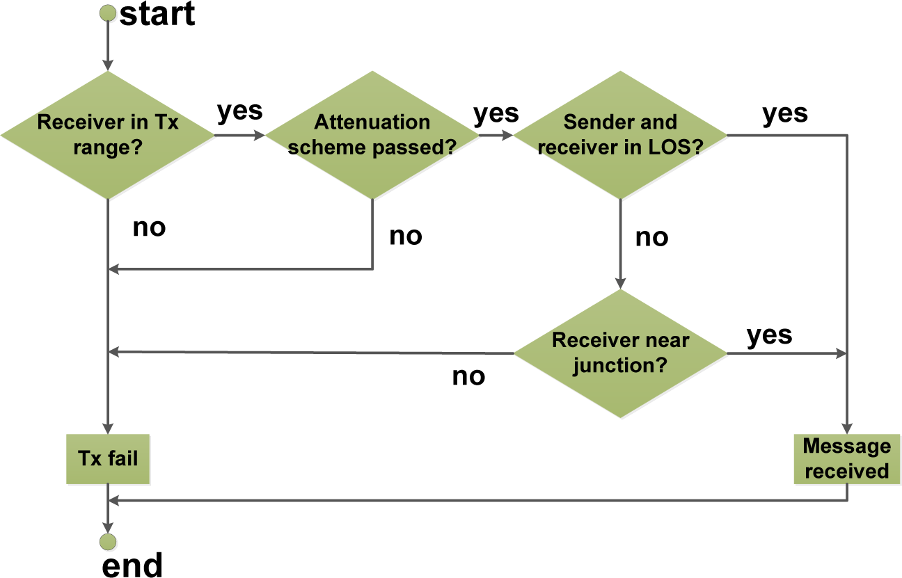
A network simulator follows the logic of the protocol stack. This is, a set of modules defines the behavior of a node during the simulation. For a wireless node, the first two modules represent the wireless communication channel and the physical layer, which are the most relevant for the objective of our study.

Channel module: This is in charge of computing the packet signal attenuation caused by the distance. This attenuation is typically called path loss or large-scale fading. It considers the attenuation caused by the presence of buildings. Then, the module introduces a variability effect in the computed power, which is called small-scale fading or just fading. Fading simulates effects, like reflectionand scattering.

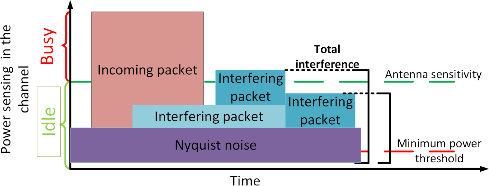
If the power computed in the reception of a packet is lower than a minimum threshold, then the packet is discarded and it is not processed by the physical simulator’s module. This threshold is typically obtained as a small fraction of the Nyquist noise associated with the channel (see Figure 6).

Physical layer module: When a packet is received by this module, it is checked against the antenna sensitivity. If the power of the incoming packet is lower than the antenna sensitivity, then it is considered interference for other packets received during their duration. Otherwise, the packet is received, and its error probability is evaluated to determine if it was correctly demodulated. Multiple incoming packets with low power are grouped to get the total interference of the channel, as shown in Figure 6. In this work, we employ the analytical packet error model proposed in [14], which considers signal to interference and noise ratio (SINR), channel capacity and packet length to decide if a packet is erroneous. An additional task of the physical module is setting the state of the channel as busy or idle according to the sensed power compared to the antenna sensitivity level.

4.2. Characterization of the Application Scenario

The authors of [15] provide a classification of vehicular applications and their communication requirements. These categories are: safety, vehicular traffic efficiency and infotainment applications.

All of the efficiency-oriented applications (e.g., air pollution, noise level monitoring, etc.) require a continuous monitoring phase of the streets and city conditions. Our application scenario assumes traffic data generated by an efficiency application during the phase of collecting data only. The characteristics of the traffic are:

• Vehicles obtain data from their sensors; they process such data and generate constant-length packets.
• The packets are sent to the closest access point (AP). This is unicast and unidirectional traffic, since the information is useful only to the authority.
• This kind of applications does not have important delay constraints as the safety related ones, so it is suitable to transport its traffic by delay-tolerant protocols.

4.3. Description of Simulation Scenarios

The simulation scenario consists of a multi-hop VANET, where we analyzed the performance of the channel modeling techniques described in Section 3. We used the Multi-Metric Map aware (MMMR)routing protocol [11], which is based on Greedy Perimeter Stateless Routing (GPSR) [16]. MMMR is a delay-tolerant protocol that improves the next forwarding node decision by employing four metrics; the distance to the destination, the vehicle density, the vehicle trajectory and the available bandwidth. This multi-metric parameter is obtained by each node, and it is used to find the neighboring node that is the candidate for being the next forwarding node. The scheme is self-configuring and able to adapt to the changing vehicle density in real time.

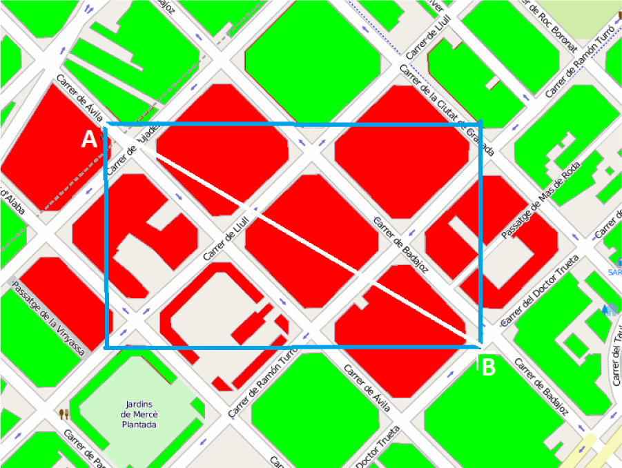
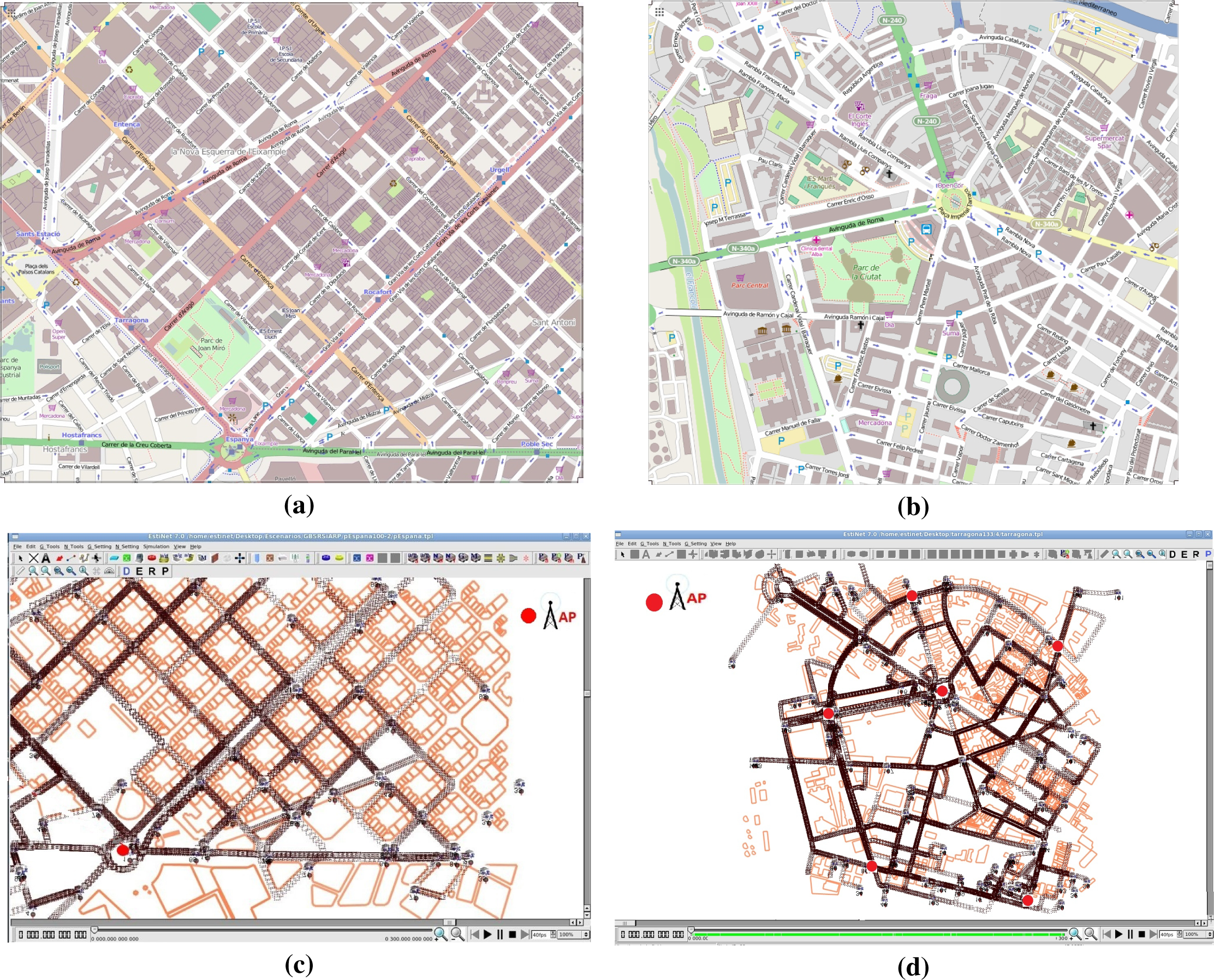
We carried out several simulations using the Estinet Network Simulator and Emulator [17]. Estinet includes the standard IEEE 802.11p and a simple and accurate way of designing VANET realistic scenarios. We used two real city areas of 1.5 and 2 km², obtained from the example district of Barcelona and the downtown district of Tarragona (see Figure 7), to evaluate two urban areas formed by streets with different densities of crossroads and buildings. In our scenarios, the Barcelona area has almost 1.3-times per square kilometer more streets and junctions than the Tarragona area. Furthermore, The example district of Barcelona has a high density of buildings compared to downtown Tarragona, specifically around four-times higher for the selected areas. Seeking to simulate a realistic scenario, the mobility model was obtained from CityMob for Roadmaps (C4R) [19], which is a mobility generator that uses the Simulation of Urban MObility (SUMO)engine [20]. C4R is able to import maps directly from OpenStreetMap [6] and to generate Network Simulator 2 (NS-2) compatible traces. C4R considers random origins and destinations for each vehicle. These points are located with higher probability in areas specified by the user. The path for a specific start and end point is computed through Dijkstra’s algorithm in a directed graph (as a GPS-based navigation system computes a route). SUMO provides a realistic driver behavior in the route followed by a car during a movement simulation. We exported the NS-2 traces to Estinet, including the building information (orange lines, see Figure 7) using our own translating software, available at www.lfurquiza.com/research/estinet [18].

The scenarios also consist of fixed nodes, which are henceforth called access points or APs. The AP enables the connection, directly or by using multiple hops, to the services in the network. The Barcelona scenario only includes one AP (see Figure 7c), while the Tarragona area has six access points (see Figure 7d). We considered four vehicle densities of 67, 100, 133 and 167 cars per km². Each of these densities could represent different situations of a day; for instance, early morning, night, morning/afternoon and rush hour. The objective of using four arbitrary different densities is to test if the difference among the results coming from the models depends on the density of the scenario. A high vehicle density helps to avoid discarding packets, since a suitable next forwarding hop would surely be always available; however, data transmissions would be more prone to interference.

Each node during the simulations sends 1000-byte packets to the destination APs, during 300 s. In the case of Barcelona, the inter-packet time follows a uniform distribution between 2 and 6 s that has a mean of 4 s. On the other side, in the Tarragona scenario, we consider that this time is exponentially distributed with a mean of 4 s, but truncated between 1 and 10 s.

All of the results are presented with confidence intervals (CI) of 95%, obtained from ten simulations per each density value and attenuation model using ten different movement traces. This means that we generated ten different movement traces per density and scenario. We use each of them to evaluate the three attenuation models.

Table 1. Simulation settings.

Parameter	Value
Map Zone	Example District of Barcelona	Downtown of Tarragona
Area	1.5 km × 1 km	1.6 km × 1.3 km
Number of junctions	712 (475 × km2)	783 (373 × km2)
Number of streets (edges)	920 (613 × km2)	993 (472 × km2)
Number of buildings (polygons)	2216 (1477 × km2)	720 (346 × km2)
Number of nodes	100, 150, 200 and 250 vehicles	133, 200, 266 and 333 vehicles
Inter-packet generation time	t~U(2,6) s E(t) = 4 s	t~Exp(mean = 4, min = 1, max = 10) s
Maximum packet size	1000 bytes
Path loss model	Empirical model of IEEE 802.11p radio shadowing [5]
	• Realistic [5] α = 9db/wall β = 0.4db/m
Building models	• Total block of signal
	• Pre-computed attenuation (Figure 5b) Step = 3
Fading model	Ricean (LOS) and Rayleigh (not in LOS)
Power transmission	23 dbm
Receiving sensing	−82 dbm (~ 400 m in LOS)
Mobility generator	SUMO [20] / C4R [19]
MAC specification	IEEE 802.11p
Bandwidth	6 Mbps
Simulation time	300 s
Routing protocol	MMMR [11]
GPS precision	10 m

summarizes the main simulation settings.

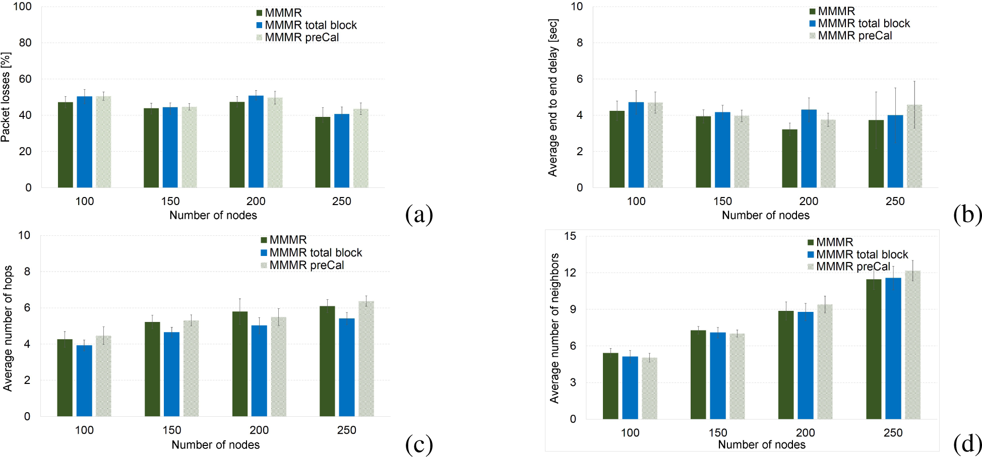
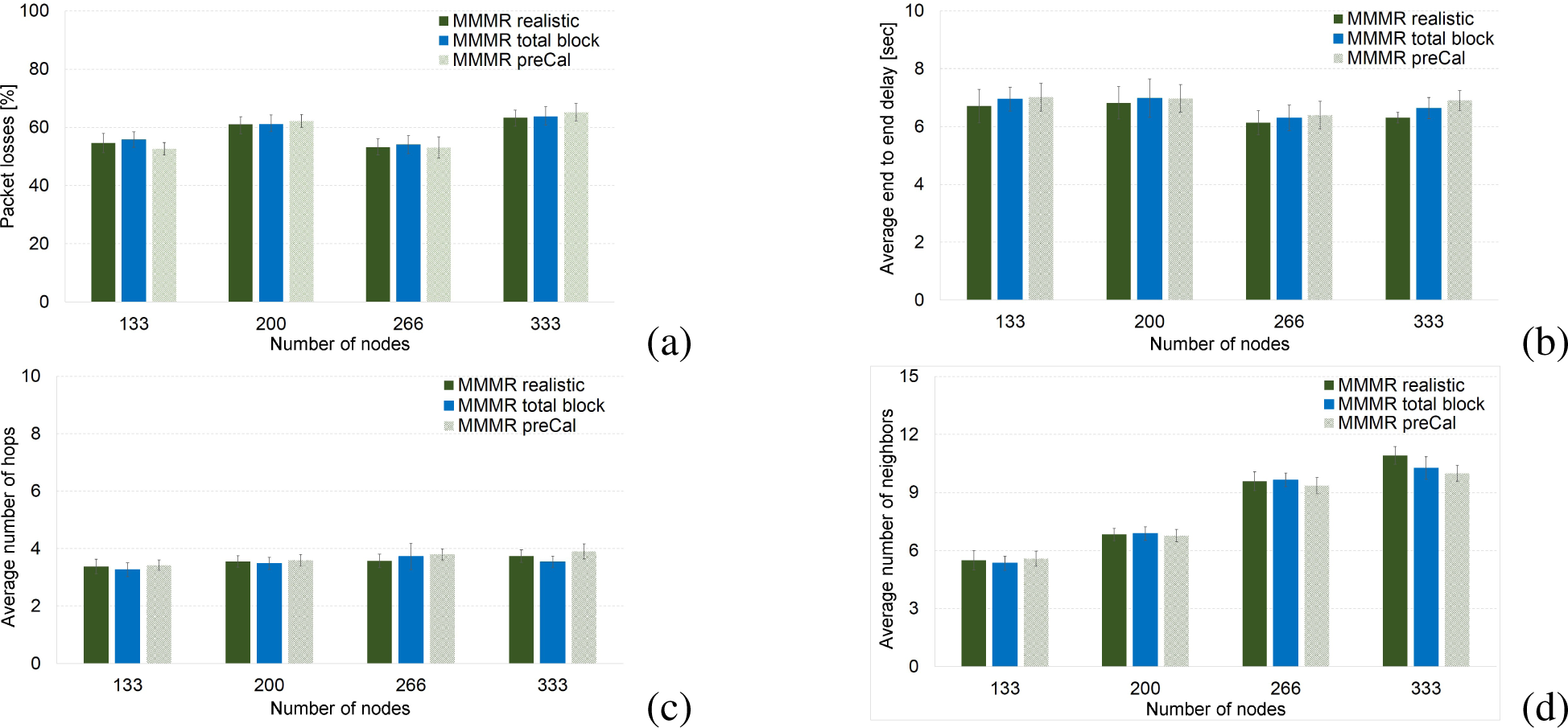
4.4. Simulation Results

In this section, we present some results from comparing the simulations of the three aforementioned attenuation models: realistic, total blockage of signal and pre-computed attenuation. The evaluation is focused on four widely-used metrics applied to the performance analysis of VANET routing protocols. These metrics are the percentage of packet losses, average delay, average number of hops and average number of neighbors. Figures 8 and 9 illustrate these results for the four node densities in the two scenarios.

The mixed ANOVA statistical test [21] was employed to check if the performance metrics differences among attenuation models depends on the vehicle density in the evaluated area. There might be a relationship since a great number of nodes may generate more collisions and higher levels of interference. We use mixed ANOVA, because for each vehicle density, the same ten vehicle movements were used to test the attenuation models. For mixed ANOVA, our data are organized into twelve groups that are obtained by combining the three building attenuation models with the four vehicle densities in the simulation. All groups have the same number of elements, which allows one to have a balanced test. The outcome of the statistical test is a probability called the p-value, which is compared with a threshold named the significance level. If the p-value is lower than the significance level, then the performance results of the system are related to both the attenuation model and the vehicle density.

The p-values, which we obtained from checking the dependency between the attenuation model and the vehicle density, are depicted in

Table 2. p-Values from Mixed Analysis of Variance (ANOVA) test for the relation between the attenuation model and vehicle density. (a) Barcelona scenario. 1 AP. Uniformly distributed traffic; (b) Tarragona scenario. 6 APs. Exponentially distributed traffic. ^*Degrees of freedom correction applied, because of the sphericity assumption violation.

Performance Metric	F Value	df	p-Value	Partial η2	Is It Significant (p-Value < 0.05)?
Packet losses*	1.204	4.2, 50.47	0.321	0.091	NO
Average delay	1.632	6, 72	0.151	0.120	NO
Average no. of hops	1.644	6, 72	0.147	0.121	NO
Average no. of neighbors	3.833	6, 72	0.002	0.242	YES
(a)

Table 2. p-Values from Mixed Analysis of Variance (ANOVA) test for the relation between the attenuation model and vehicle density. (a) Barcelona scenario. 1 AP. Uniformly distributed traffic; (b) Tarragona scenario. 6 APs. Exponentially distributed traffic. ^*Degrees of freedom correction applied, because of the sphericity assumption violation.

Performance Metric	F Value	df	p-Value	Partial η2	Is It Significant (p-Value < 0.05)?
Packet losses	1.997	6, 72	0.077	0.143	No
Average delay	0.572	6, 72	0.751	0.041	No
Average No. of hops*	1.013	4.585, 55.02	0.415	0.078	No
Average No. of neighbors	2.657	6, 72	0.022	0.181	Yes
(b)

, where the F-ratio is the result of the F-test statistical test [22], df represents the degrees of freedom used to obtain the p-value and partial η² is a measure of the effect size. According to the results of the Mixed-ANOVA, we can conclude that there is no significant interaction between the attenuation models and the vehicle density, since the p-value is lower than 0.05 in none of the performance metrics for both scenarios, except for the average number of neighbors. Mixed ANOVA assumes that the data come from normally-distributed populations with a homogeneous variance and similar covariance and sphericity (differences between all possible pairs of groups are equal). Some of the twelve data groups of our performance results violate some of these assumptions, especially normal distribution and homogeneous variance. However, our test results can be considered reliable, because ANOVA is robust to these assumptions [23], especially under the balance number of elements in each group [24].

When there is not a significant dependency between the factors in the mixed ANOVA, as happens in our study between attenuation models and vehicle density for the percentage of packet losses, average end-to-end delay and average number of hops, the post hoc tests, i.e., repeated measures ANOVA [21], to study the attenuation model effects do not need to differentiate between the vehicle densities. On the other hand, the post hoc tests for the average number of neighbors metric have to be done for each vehicle density independently. According to mixed ANOVA results, the differences among these metrics depend on the vehicle density used in the simulation.

Due to the post hoc test (ANOVA with repeated measures), it is required to meet the same assumptions of mixed ANOVA, and even when this test is robust to violations of these assumptions, we decided to apply the equivalent non-parametric tests to assess the difference among the attenuation models, because our data conform to their requirements. For our data, both kinds of tests, parametric and non-parametric, agree with the same decision in all of the post hoc tests performed in this work. There is not a well-accepted non-parametric statistical test equivalent to mixed ANOVA.

Table 3. p-Values from the Friedman test to determine the effect of the building attenuation model. (a) Barcelona scenario: one AP; uniformly-distributed traffic. (b) Tarragona scenario: six APs; exponentially-distributed traffic.

Performance Metric	Vehicle Density	Test Statistic	df	p-Value(br)2 Sides	Is It Significant p-Value < 0.05?
Packet losses	all together	10.55	2	0.005	Yes
Average delay	all together	18.95	2	0.0001	Yes
Average No. of hops	all together	42.35	2	0.0001	Yes
	67	9.8	2	0.007	Yes
Average No. of neighbors	100	2.6	2	0.273	No
	133	9.614	2	0.008	Yes
	166	9.614	2	0.008	Yes
(a)

Table 3. p-Values from the Friedman test to determine the effect of the building attenuation model. (a) Barcelona scenario: one AP; uniformly-distributed traffic. (b) Tarragona scenario: six APs; exponentially-distributed traffic.

Performance Metric	Vehicle Density	Test Statistic	df	p-Value(br)2 Sides	Is It Significant p-Value < 0.05?
Packet losses	all together	1.55	2	0.461	No
Average delay	all together	10.4	2	0.006	Yes
Average No. of hops	all together	22.05	2	0.0001	Yes
	67	5.6	2	0.061	No
Average No. of neighbors	100	1.4	2	0.497	No
	133	4.66	2	0.097	No
	166	5.59	2	0.061	No
	all together	4.899	2	0.086	No
(b)

shows the p-values obtained from the Friedman test [22], which is the non-parametric version of ANOVA for repeated measures. It is used to know if there are statistically significant differences among the building attenuation models.

As the reader can notice, none of the p-values of Table 3a (Barcelona scenario) are higher than the significance threshold of 0.05, except the average number of neighbors for a vehicle density of 100 cars/km². Hence, this means that there is a statistically significant difference among the distribution of the results obtained when the simulation uses different building attenuation models, excluding the average number of neighbors for a vehicle density of 100 cars/km². All of these differences, i.e., the percentage of packet losses, average end-to-end delay and average number of neighbors, are not detected in the performance results of the Tarragona scenario. It can be seen in Table 3b that the p-values show significant differences in average delay and average number of hops. We would like to point out that even when the p-value of mixed ANOVA (to test the interaction between the attenuation models and the vehicle density in the Tarragona scenario; see Table 2b) is significant, the Friedman tests performed per vehicle density do not detect any difference in any of the cases. One reason that explains this result is that the effect size of the interaction is lower in the Barcelona scenario.

We used a pairwise comparison to determine the models among which there exists a difference in terms of the performance results.

Table 4. p-Values of Wilcoxon signed rank test for a pairwise comparison of the building attenuation model effect. (a) Barcelona scenario. 1 AP. Uniformly distributed traffic; (b) Tarragona scenario 6 APs. Exponentially distributed traffic.

Performance Metric	Pairwise	Standardized Test Statistic	p-Value 2 Sides	Is the Difference Significant (p-Value < 0.017)?	Median of Differences
Packet losses	Realistic, total block	2.983	0.003	Yes	−2.3780%
	Realistic, pre-computed	3.602	0.0001	Yes	−3.0614%
	Total block, pre-computed	1.423	0.155	No	−0.91%
Average delay	Realistic, total block	4.019	0.0001	Yes	−0.5310 s
	Realistic, pre-computed	3.360	0.001	Yes	−0.4391 s
	Total block, pre-computed	−0.565	0.572	No	0.0136 s
Average number of hops	Realistic, total block	−5.309	0.0001	Yes	0.66 hops
	Realistic, pre-computed	1.559	0.119	No	−0.11 hops
	Total block, pre-computed	5.242	0.0001	Yes	−0.78 hops
Average number of neighbors 67	Realistic, total block	−2.091	0.037	No	0.285 nodes
	Realistic, pre-computed	−2.599	0.009	Yes	0.485 nodes
	Total block, pre-computed	−0.153	0.878	No	−0.075 nodes
Average number of neighbors 133	Realistic, total block	−0.816	0.415	No	0.06 nodes
	Realistic, pre-computed	1.734	0.83	No	−0.315 nodes
	Total block, pre-computed	2.499	0.012	Yes	−0.565 nodes
Average number of neighbors 166	Realistic, total block	−2.803	0.005	Yes	0.39 nodes
	Realistic, pre-computed	1.020	0.308	No	−0.185 nodes
	Total block, pre-computed	2.497	0.013	Yes	−0.525 nodes
(a)

Table 4. p-Values of Wilcoxon signed rank test for a pairwise comparison of the building attenuation model effect. (a) Barcelona scenario. 1 AP. Uniformly distributed traffic; (b) Tarragona scenario 6 APs. Exponentially distributed traffic.

Performance Metric	Pairwise	Standardized Test Statistic	p-Value 2 Sides	Is the Difference Significant	Median of Differences
Average delay	Realistic, total block	2.285	0.022	No	−0.3084 s
	Realistic, pre-computed	3.428	0.001	Yes	−0.2893 s
	Total block, pre-computed	0.82	0.412	No	−0.0919 s
Average number of hops	Realistic, total block	−2.393	0.016	Yes	0.836 hops
	Realistic, pre-computed	2.796	0.005	Yes	−0.1464 hops
	Total block, pre-computed	3.549	0.0001	Yes	−0.2651 hops
(b)

shows the p-values for this comparison by using the Wilcoxon statistical test [22]. We employed the Bonferroni correction in these pairwise comparison. That is, the new significance threshold is 0.017, obtained by dividing 0.05 by the number of options compared (i.e., 0.05/3).

From Table 4a for the Barcelona scenario, we can see that the results of the performance metrics are significantly different (see Rows 1,4 and 7 and 16) if we model the effects of building presence as the total absence of communication, compared with the results obtained with a realistic channel model, specifically designed for VANETs. Comparison between these two models in the Tarragona scenario shows significant differences in the average number of hops (see the fourth row in Table 4b). Moreover, the total signal blocking always shows the most conservative behavior. This can be noticed in the values of the column of the median of the differences in both Table 4a and 4b). This behavior makes total sense, since this model involves nodes sensing fewer neighbors (vehicles cannot detect nodes behind obstacles in any case under the total-blockage attenuation model). Additionally, the absence of communications avoids the construction of paths that in a realistic approach may be feasible. Consequently, packets need to be stored in nodes for longer periods until finding a forwarding node, so the percentage of packet losses increases due to the timeouts. Notice that in the Barcelona scenario, the differences in the average number of neighbors are only detected in the high density case.

This behavior is explained by the communications between obstructed nodes not being the rule, and most of them entail high error probabilities. As a consequence, the differences in the performance metrics are small in our simulations scenarios, as is shown in the column of the reported medians.

Regarding the comparison between the realistic channel model and the pre-computed attenuation approach, it can be noticed (see Rows 8, 14 and 17 in Table 4a) that there is no statistically significant difference in the average number of hops or neighbors. Nevertheless, there are discrepancies in the percentage of packet losses and in the average end-to-end delay (see Rows 2, 5 of Table 4a). Notice that there is a difference in the average number of neighbors for a density of 67 vehicles/km². Similar results are obtained from Tarragona scenario (See Table 4b), but in this case, there are only significant differences in the average end-to-end delay and the average number of hops.

For both scenarios, the median of the pre-computed attenuation performance results are not so far from the medians in the realistic scenario. The presence of differences between the aforementioned models is a consequence of the discretization process done in the pre-computed attenuation approach.

Lastly, total blockage and pre-computed building attenuation models are compared in order to get an idea of the existing differences between these approaches and the realistic channel model. The reader can observe from Table 4a in the case of the Barcelona scenario and Table 4b for Tarragona that there are statistical differences in the average number of hops of a packet when traveling to reach the access point. Furthermore, differences in the average number of nodes between these two models appear only for the two highest densities applied in this work (133 and 166 nodes/km²) in the Barcelona scenario. Hence, the results obtained with these two models could be similar, at least in the percentage, to the packet losses and delay.

To conclude this section, we summarize the major features and results drawn from our evaluation:

• We have simulated three building attenuation models used in the literature for VANETs (i.e., realistic, total blocking of the signal and the precomputed attenuation model) under two realistic urban scenarios that have different vehicle densities, junctions and buildings. The study considered four different vehicle densities with ten different mobility traces per density. Moreover, different probability distributions for traffic generation were used in each urban scenario.
• The results of statistical tests carried out with four performance metrics (percentage of packet losses, end-to-end delay, average number of hops and neighbors) show differences when employing different attenuation models.
• A complete attenuation of the signal due to the presence of buildings, and pre-computed attenuation models in our simulations can be considered for both scenarios as pessimistic bounds for all performance metrics.
• We did not find that the differences in the performance metrics are affected by the vehicle density employed during the simulation, except in the case of the average number of neighbors. This metric does not differ from the realistic one with intermediate vehicle density scenarios.

These are promissory results, because they lead to the idea of using the total signal attenuation model or pre-computed attenuation files when a realistic attenuation model is difficult to use; for instance, for map areas where building information is not available and a complete blockage outside the street has to be assumed. Pre-computed attenuation files would be a good alternative when scenarios involve a medium or high data traffic load, especially in preliminary studies. Such scenarios require that algorithms to calculate the level of attenuation caused by buildings are executed too many times. This can cause important time consumption due to the number of operations, even when such algorithms are efficient.

5. Conclusions

A statistical analysis has been performed in this work about the simulation of multi-hop vehicular ad hoc networks and, particularly, on how their performance metrics vary according to the attenuation effects obtained by modeling the presence of buildings in a VANET scenario. Our study compares three strategies to model the influence of buildings on the communication between vehicles. These strategies model this influence as the full attenuation of the communication signals, as a number of offline computed values of attenuation and as an inexpensive and accurate realistic propagation scheme [5].

The results we obtained support that the performance metric scores depend on the building attenuation model used in the simulations. Hence, the research community should use a realistic propagation model when possible.

The differences in the performance reached with the realistic model, compared with the other two models, are at the maximum 3% for the percentage of packet losses and 0.5 s for end-to-end delay in our two different simulation scenarios, for the traffic-efficiency application tested in this work. Furthermore, we could not find any statistical relationship between the vehicle density in the scenario (which may include a higher data traffic load) and the building attenuation model used, except by the average number of neighbors.

Obstructed communications with higher capacity channels are less probable, and consequently, the resulting gap between a realistic building attenuation model and a total blockage of the signal should decrease when using higher capacity channels. Future work may include testing the different channel capacities available in IEEE 802.11p in order to find out if the assumption of total attenuation differs from the realistic scenario for any channel capacity and average rate in the scenario. Furthermore, tests to empirically obtain the curve of the differences among the models in different types of scenarios is in the future work plan. Additionally, we are interested in testing different ways to map the continuous time into the discrete time for the offline attenuation files. Furthermore, the impact of the discretization step used to build the attenuation file (that currently has a size of 110 MB for a simulation of 300 seconds with 250 nodes) may be measured in a future study, since there would be a trade-off between accuracy and file size.

Another future work might involve assessing the differences among the three techniques explained in this paper, but applying them to delay sensitive applications, like dissemination of warning messages for safety purposes. This could be done by using more appropriate metrics, such as jitter, time to cover an area, number of notified vehicles, etc. We are planning to use real mobility traces, such as the ones provided in [25] or [26], to leverage a trustworthy evaluation of this kind of applications, especially in the analysis of how long and how fast an emergency message can be spread over a large area.

References

1. Hartenstein, H.; Laberteaux, K.; Ebrary, I. VANET: Vehicular Applications and Inter-Networking Technologies; John Wiley & Sons, Ltd.: Chichester, UK, 2010. [Google Scholar]
2. Scopigno, R.; Cozzetti, H. Signal Shadowing in Simulation of Urban Vehicular Communications. Proceedings of the 2010 6th International Conference on Wireless and Mobile Communications (ICWMC), Valencia, Spain, 2010; pp. 131–138.
3. Nagel, R.; Eichler, S. Efficient and Realistic Mobility and Channel Modeling for VANET Scenarios Using OMNeT++ and INET-framework. Proceedings of the 1st International Conference on Simulation Tools and Techniques for Communications, Networks and Systems & Workshops (Simutools ’08), Institute for Computer Sciences, Social-Informatics and Telecommunications Engineering, Brussels, Belgium, 2008; pp. 89:1–89:8.
4. Chia, S.T.S.; Snow, P. Characterising radio-wave propagation behaviour at 1700 MHz for urban and highway microcells. Proceedings of the Micro-Cellular Propagation Modelling, IEEE Colloquium, London, UK, 1992; pp. 11:1–11:4.
5. Sommer, C.; Eckhoff, D.; German, R.; Dressler, F. A computationally inexpensive empirical model of IEEE 802.11p radio shadowing in urban environments. Proceedings of the 2011 Eighth International Conference on Wireless On-Demand Network Systems and Services (WONS), Bardonecchia, Italy, 26–28 January 2011; pp. 84–90.
6. Open Street Maps. Available online: http://www.openstreetmap.org/ accessed on 28 October 2014.
7. Wang, S.Y.; Wang, P.F.; Li, Y.W.; Lau, L.C. Design and implementation of a more realistic radio propagation model for wireless Vehicular Networks over the NCTUns network simulator. Proceedings of the 2011 IEEE Wireless Communications and Networking Conference (WCNC), Cancun, Quintana Roo, Mexico, 28–31 March 2011; pp. 1937–1942.
8. Martinez, F.J.; Fogue, M.; Toh, C.K.; Cano, J.C.; Calafate, C.T.; Manzoni, P. Computer Simulations of VANETs Using Realistic City Topologies. Wirel. Pers. Commun. 2013, 69, 639–663. [Google Scholar]
9. Gozalvez, J.; Sepulcre, M.; Bauza, R. Impact of the radio channel modelling on the performance of VANET communication protocols. Telecommun. Syst. 2010, 50, 149–167. [Google Scholar]
10. Urquiza, L.; Tripp, C.; Martin, I.; Aguilar, M. Propagation and Packet Error models in VANET simulations. IEEE Latin Am. Trans. 2014, 12, 499–507. [Google Scholar]
11. Tripp-Barba, C.; Urquiza-Aguiar, L.; Igartua, M.A.; Rebollo-Monedero, D.; Mezher, A.M.; de la Cruz Llopis, L.J.; Aguilar-CalderÃşn, J.A. A Multimetric, Map-Aware Routing Protocol for VANETs in Urban Areas. Sensors 2014, 14, 2199–2224. [Google Scholar]
12. Lochert, C.; Mauve, M. Geographic routing in city scenarios. ACM SIGMOBILE Mob. Comput. Commun. Rev. 2005, 9, 69–72. [Google Scholar]
13. Mezher, A.M.; Oltra, J.J.; Aguiar, L.U.; Paredes, C.I.; Barba, C.T.; Igartua, M.A. Realistic Environment for VANET Simulations to Detect the Presence of Obstacles in Vehicular Ad Hoc Networks. Proceedings of the 11th ACM Symposium on Performance Evaluation of Wireless Ad Hoc, Sensor, & Ubiquitous Networks PE-WASUN ’14, ACM, Montreal, QB, Canada, 21–26 September 2014; pp. 77–84.
14. Abrate, F.; Vesco, A.; Scopigno, R. An Analytical Packet Error Rate Model for WAVE Receivers. Proceedings of the 2011 IEEE Vehicular Technology Conference (VTC Fall), San Francisco, USA, 5–8 September 2011; pp. 1–5.
15. Caloca, C.; Garcia Macias, J.A. Adaptive Solutions in Multihop Communication Protocols for Vehicular Ad Hoc Networks. In Advances in Vehicular Ad-Hoc Networks: Developments and Challenges; Watfa, M., Ed.; IGI global: Hershey, PA, USA, 2010; pp. 301–322. [Google Scholar]
16. Karp, B.; Kung, H.T. GPSR Greedy perimeter stateless routing for wireless networks. Proceedings of the 6th Annual International Conference on Mobile Computing and Networking—MobiCom ’00, New York, NY, USA, 6–11 August 2000; pp. 243–254.
17. Estinet-Technologies. EstiNet Network Simulator and Emulator. Available online: http://www.estinet.com/products.php?lv1=1&sn=2 accessed on 28 October 2014.
18. Software to VANET simulations. Available online: http://www.lfurquiza.com/research/estinet accessed on 28 October 2014.
19. Fogue, M.; Garrido, P.; Martinez, F.J.; Cano, J.C.; Calafate, C.T.; Manzoni, P. A Realistic Simulation Framework for Vehicular Networks. Proceedings of the 5th International ICST Conference on Simulation Tools and Techniques Simutools ’12, Brussels, Belgium, March 2012; pp. 37–46.
20. Krajzewicz, D.; Erdmann, J.; Behrisch, M.; Bieker, L. Recent Development and Applications of SUMO—Simulation of Urban MObility. Int. J. Ad. Syst. Meas. 2012, 5, 128–138. [Google Scholar]
21. Maxwell, S.E.; Delaney, H.D. Designing Experiments and Analyzing Data: A Model Comparison Perspective; Psychology Press: London, UK, 2004; Volume 1. [Google Scholar]
22. Sheskin, D. Handbook of Parametric and Nonparametric Statistical Procedures, 2nd ed; Chapman & Hall CRC: Boca Raton, FL, USA, 2000. [Google Scholar]
23. Lewicki, P.; Hill, T. Statistics: Methods and Applications; online ed.; Statsoft: Tulsa, OK, USA, 2013. [Google Scholar]
24. Wilcox, R. Robustness in ANOVA. In Applied Analysis of Variance in Behavioral Science. Statistics: Textbooks and monographs; Marcel Dekker: New York, NY, USA, 1993; pp. 345–364. [Google Scholar]
25. Uppoor, S.; Trullols-Cruces, O.; Fiore, M.; Barcelo-Ordinas, J.M. Generation and Analysis of a Large-Scale Urban Vehicular Mobility Dataset. IEEE Trans. Mob. Comput. 2014, 13, 1061–1075. [Google Scholar]
26. Pigné, Y.; Danoy, G.; Bouvry, P. A Vehicular Mobility Model Based on Real Traffic Counting Data. In Communication Technologies for Vehicles of Lecture Notes in Computer Science series; Strang, T., Festag, A., Vinel, A., Mehmood, R., Rico Garcia, C., Röckl, M., Eds.; Springer: Berlin Heidelberg, Germany, 2011; Volume 6596, pp. 131–142. [Google Scholar]
Figure 1. Discrete positions of a vehicle in a Manhattan scenario proposed in [2].
Electronics 04 00037f1
Figure 2. Detection of relevant building influence in the transmission process between nodes A and B. Red buildings are considered to have a relevant influence. We use a zone map of Barcelona, Spain.
Electronics 04 00037f2
Figure 3. Flowchart of the visibility model proposed in [8].
Electronics 04 00037f3
Figure 4. Packet error probability (PEP) behavior in an obstructed communication scenario between two vehicles near a corner. Empirical IEEE 802.11p channel model. Channel Capacity= 6 Mbps. Antenna sensitivity = −82 dbm. (a) Near-line-of-sight (NLoS) scenario at a corner; (b) PEP vs. distance.
Electronics 04 00037f4
Figure 5. Pre-computed attenuation file format with its corresponding localization value algorithm used in this work. (a) Output format; (b) Position computation algorithm.
Electronics 04 00037f5
Figure 6. State of the channel and interference management of a wireless channel for a node in a network simulator [10].
Electronics 04 00037f6
Figure 7. Simulation scenarios from two cities of Catalonia, Spain. (a) Example district of Barcelona from OSM; (b) downtown area of Tarragona from OSM; (c) barcelona simulated scenario with an access point (AP); buildings from OpenStreetMap are included. (d) Tarragona simulated scenario with six APs; buildings from OpenStreetMap are included.
Electronics 04 00037f7
Figure 8. Building attenuation model comparison (Barcelona scenario) (CI 95%). (a) Percentage of packet losses; (b) average end-to-end delay; (c) average number of hops; (d) average number of neighbors.
Electronics 04 00037f8
Figure 9. Building attenuation models comparison (Tarragona scenario) (CI 95%). (a) Percentage of packet losses; (b) average end-to-end delay; (c) average number of hops; (d) average number of neighbors.
Electronics 04 00037f9