Quantifying AI Model Trust as a Model Sureness Measure by Bidirectional Active Processing and Visual Knowledge Discovery

Abstract

Trust in machine-learning models is critical for deployment by users, especially for high-risk tasks such as healthcare. Model trust involves much more than performance metrics such as accuracy, precision, or recall. It includes user readiness to allow a model to make decisions. Model trust is a multifaceted concept commonly associated with the stability of model predictions under variations in training data, noise, algorithmic parameters, and model explanations. This paper extends existing model trust concepts by introducing a novel Model Sureness measure. Some alternatively purposed Model Sureness measures have been proposed. Here, Model Sureness quantitatively measures the model accuracy stability under training data variations. For any model, this is carried out by combining the proposed Bidirectional Active Processing and Visual Knowledge Discovery. The proposed Bidirectional Active Processing method iteratively retrains a model on varied training data until a user-defined stopping criterion is met; in this work, this criterion is set to a 95% accuracy when the model is evaluated on the test data. This process further finds a minimal sufficient training dataset required for a model to satisfy this criterion. Accordingly, the proposed Model Sureness measure is defined as the ratio of the number of unnecessary cases to all cases in the training data along with variations of these ratios. Higher ratios indicate a greater Model Sureness under this measure, while trust in a model is ultimately a human decision based on multiple measures. Case studies conducted on three benchmark datasets from biology, medicine, and handwritten digit recognition demonstrate a well-preserved model accuracy with Model Sureness scores that reflect the capabilities of the evaluated models. Specifically, unnecessary case removal ranged from 20% to 80%, with an average reduction of approximately 50% of the training data.

1. Introduction

1.1. Motivation

Domain experts’ and users’ trust in machine-learning (ML) models is crucial for deployment, especially in high-risk fields like healthcare and automotive systems [1,2,3,4,5,6]. The resultant “trust gap” is important in contemporary industrial settings [7], in areas where ML models are increasingly tasked with controlling complex and commonly stochastic processes. Here, high-fidelity physics-based simulations can be too slow or expensive to run in practice. Therefore, data-driven deep-learning architectures are now routinely employed, for example, in real-time quality monitoring in additive manufacturing [8]. As such, “black-box” models are becoming integral components of process control and quality assurance systems. However, there remains a pressing and largely unresolved need for rigorous methods to quantify models in terms of reliability and trustworthiness. Because trust is a human activity, such measures only support human evaluation.

Trust in ML models goes beyond metrics like accuracy, precision, or recall. It also involves user confidence in a model’s accuracy reliability, comfort with understanding its behavior, and willingness to rely on its decisions [3,4]. Trust often depends on a model’s structural stability (i.e., learned patterns) and consistent accuracy across various configurations and training data. These variations include changes to the training data, types of noise in the data, learning algorithm (hyper-)parameters, and model explanations. Several concepts of ML model trust have been proposed. This paper expands on them by introducing a Model Sureness (MS) measure that aligns with key dimensions in trustworthiness frameworks.

The Model Sureness measure studied here quantifies how training data variations affect the stability of a chosen algorithm’s yielded model’s accuracy, for example, an algorithm that consistently yields high-accuracy models even when trained on highly varied subsets of the data. Such models exhibit high training-data Model Sureness, a prerequisite for being regarded as highly trustworthy [5]. Other Model Sureness measures for variations beyond training data are outside this study’s scope; however, only the definition of the model success criterion would change.

The Model Sureness analysis may also show that a model’s accuracy is extremely sensitive to variations in the training data. Such sensitivity undermines trust in both the model and the training data used to construct it. Addressing this issue may require modifying both the training data and the selected feature set. Changes to feature selection are also beyond the scope of this study. Nevertheless, Model Sureness measures can guide such refinements by summarizing the model accuracy or any user-defined performance metric and highlighting training cases that most strongly drive model variability.

This work quantifies the sing two complementary approaches: the (1) computational Bidirectional Active Processing (BAP) and (2) interactive Visual Knowledge Discovery (VKD) approaches. For example, if a much smaller training subset yields a model with the same properties as one trained on the full dataset, the model has a high Model Sureness. Typically, a user assesses a model’s trustworthiness using only a limited subset of the available data. Thus, the observed data may misrepresent the full data distribution. Thus, inherent uncertainty motivates the Model Sureness approach.

In Figure 1a, the Model Sureness is high since the two classes are well-separated with unmixed points in the oval. In Figure 1b, the Model Sureness is low since cases in the oval mix the two classes. In this simplified 2-D example, boundary and mixed points are visually distinct. However, in high-dimensional data, points cannot be directly observed to qualitatively assess the Model Sureness without lossless visualization. In contrast, the proposed Model Sureness measure is computationally practical for high-dimensional data.

Model Sureness is defined formally and numerically later. Therefore, the difference in Model Sureness measures between the models in Figure 1a,b is expressed here in terms of training case reduction. If removing many training cases yields a similarly high-accuracy model, then the Model Sureness is high. Conversely, if removing many training cases yields a model with degraded accuracy, then the Model Sureness is low.

In Figure 1a, 90% of cases (18 out of 20) are classified correctly. Using the 10 cases outside the oval as training data yields 100% training and 80% test accuracy in the oval’s interior (8 out of 10). Conversely, using the 10 cases inside the oval as training data yields 80% training (18 out of 20) and 100% test accuracy over the oval’s exterior. However, in Figure 1b, removing cases strongly reduces the classification accuracy, yielding a lower Model Sureness. Using all 80 cases (40 red, 40 blue) for training yields a test accuracy of 90% (8 misclassifications: 4 red, 4 blue). Using only the cases outside the oval for training yields 100% training accuracy but 33.34% test accuracy inside the oval (8 misclassifications: 4 red and 4 blue out of 24). Swapping the training and test sets swaps these accuracy values.

The average accuracy of the two subsets in Figure 1a is 90%, matching the full dataset. In contrast, the average accuracy of the two subsets from Figure 1b is only 66.67%, compared to 90% for all data. For Figure 1a, two subsets with 50% of cases achieve a ≥80% accuracy; for Figure 1b, only one does. These examples show that measuring Model Sureness requires testing multiple smaller subsets through repeated experiments.

Noise in data is well known to obscure patterns and degrade model accuracy. Model Sureness identifies models that maintain a stable accuracy despite noisy data. Models with stable properties beyond accuracy are beyond this work’s scope. The proposed approach trains models sequentially. Each successive model is trained on updated training data. Data updates add or remove cases until models reach the user-specified test accuracy. This process also identifies minimal training-data subsets for reliable model accuracy.

The order of adding or removing cases from training data can significantly impact the resulting models. Exhaustively testing all training case combinations is combinatorially infeasible. Therefore, we reduce the computational cost by using limited repeated stratified sampling to preserve the class balance and explore multiple plausible training datasets. Hence, this process is stochastic across experimental repetitions. For adding cases, we sample from the current data subset, and, for removing cases, from the full training set.

Noisy cases in training data often hide meaningful structure with non-representative patterns. In our case studies, the proposed process removed 20–80% of noisy or redundant cases, averaging a 50% data reduction. This approach reduces data use and identifies truly representative cases for model building. This process is conceptually aligned with the approach in [6] that found worst-case training cases via Visual Knowledge Discovery. This often enhances purely analytical approaches [9,10,11,12,13]. Reducing the number of training cases used is particularly relevant for large datasets, such as the MNIST handwritten digit image dataset [14], which contains 60,000 training cases in a 28 × 28-pixel image with grayscale values of 0–255 for a 784-dimensional feature space with 256⁷⁸⁴ possible cases. Case Study 5.3 examines this data and demonstrates that models with a comparable accuracy on the 10,000 test cases can be obtained from subsets of only 2500–9600 cases instead of the full dataset, resulting in substantial computational benefits.

1.2. Challenges and Opportunities

Reducing the number of training cases may not always be successful. A large drop in accuracy after removing certain training cases suggests those cases are highly representative of their class or crucial for capturing class patterns. Impactful cases can be assessed through visual inspection using lossless visualization by comparing them to their nearest neighbors [10]. If accuracy barely changes when these cases are added or removed, they are probably not representative of the class structure and may instead be noise.

Any aspect of the model pipeline—data attributes, parameters, or design choices—can be varied as an indicator of stability and trust, and to identify relevant attribute subsets. For example, this process can identify stable, relevant subsets of attributes. Moreover, model trust depends on underlying assumptions at model construction. Unfortunately, users often overlook these assumptions, which need scrutiny in high-risk fields like healthcare.

ML often assumes the distribution of unseen data matches the distribution of the training data, limiting its use in trust-critical tasks. While this assumption may be reasonable at the population level, it fails to account for case-specific variability and outliers. This limitation matters most in high-risk tasks, where single errors carry high costs.

Crucially, not all data cases are known in advance, and new outliers may emerge. Moreover, prior research shows that atypical cases can behave fundamentally differently and may disproportionately impact model performance compared to typical cases [6]. The proposed Model Sureness measure helps test such assumptions of distributional similarity between the training and unseen test data. Formally, it enables the estimation of mathematical bounds on the minimum and maximum training data sizes required for a model to achieve the desired properties, such as test dataset accuracy, as used in this work.

1.3. Summary of the Proposed Approach

The proposed approach enhances the trust analysis in ML models. It introduces the concept of Model Sureness, which measures the impact of training data variations on the model accuracy for a chosen ML algorithm. Model Sureness can be computed using either (1) the computational Bidirectional Active Processing (BAP) approach proposed in this paper, or (2) interactive Visual Knowledge Discovery (VKD) processes [9].

The BAP approach supports dataset reduction for a wide range of ML algorithms. One such example is the Generalized Iterative Classifier (GIC) framework [9,10]. These models employ Generalized Decision Trees (GDTs), which allow for non-binary decision levels. Because each GDT level depends on the structure and composition of the training data, reducing the dataset yields a cascading effect that simplifies downstream decision nodes and improves the overall interpretability of the model.

BAP offers the following key advantages over other computational methods for identifying reduced training datasets, detailed later:

(1)

Algorithm agnosticism. BAP serves as an algorithm-agnostic wrapper that finds minimal sufficient training sets, unlike many algorithm-specific methods.

(2)

Simplicity and scalability. BAP is simpler than methods that rely on additional processing or auxiliary analyses when searching for reduced training datasets, making it more scalable and highly parallelizable. Approaches that utilize extra processing during case addition or removal may identify better subsets for some specific criterion, but they can also miss superior subsets under many alternative criteria. Moreover, optimizing additional criteria requires explicit justification and introduces dependencies that limit parallelization, thus limiting scalability.

(3)

Controlled exploration of training subsets. BAP allows for explicit control over the number of cases tested at each step, reducing the risk of convergence to local minima and being able to adapt to data characteristics. This contrasts with binary search–based halving strategies and standard cross-validation schemes using fixed folds (e.g., 5-fold or 10-fold cross-validation).

Next, the interactive Visual Knowledge Discovery (VKD) approach offers added benefits through active user involvement. This enables domain expertise to guide the selection of more relevant reduced training data. Moreover, combining BAP and VKD yields complementary advantages: BAP enables efficient computation on large datasets, while VKD facilitates deeper user knowledge integration and model interpretability.

Primary novelty. This paper’s primary novelty lies in (1) linking reduced training dataset studies with ML model trustworthiness, and (2) proposing a numerical Model Sureness measure based on such datasets. This view differs from the typical dataset reduction, which mainly aims to accelerate model computation [15]. Such computationally motivated approaches have grown increasingly vital amid the spread of resource-intensive models like deep learning and large language modes.

Another key novelty is (3) linking the whole area of multiple existing methods that find smaller training datasets with the visualization of high-dimensional data and Visual Knowledge Discovery allowing (4) finding these datasets in visualization and (5) solving ML tasks with visual means, which often is impossible for large training datasets. This benefits both lossy methods (Principal Component Analysis (PCA) and t-Distributed Stochastic Neighbor Embedding (t-SNE)) and lossless methods (Parallel Coordinates (PC) and General Line Coordinates (GLC)) [11].

The remainder of this paper is organized as follows: Section 2 reviews the related work; Section 3 presents the methodology; Section 4 covers the algorithmic details; Section 5 reports case studies on the Iris [16], Wisconsin Breast Cancer [16], and MNIST handwritten digit [14] datasets; and Section 6 concludes with the discussion and future work.

2. Related Work

2.1. Model Trustworthiness as a Multidimensional Evaluation Framework

Trustworthiness in machine learning involves key dimensions that ensure models are reliable, ethical, and transparent. Fairness addresses bias and the prevention of discrimination against subgroups with widely studied metrics that measure this like demographic parity and equality of opportunity [17,18,19,20,21,22]. Robustness measures a model’s stability against noise and adversarial inputs and ensures prediction consistency under perturbations [23,24]. Confidence and calibration ensure that the predicted probabilities accurately reflect the true likelihoods, leveraging metrics like the Expected Calibration Error and Brier score [25,26,27]. Interpretability involves understanding model decisions via feature importance rankings and explanations aligned with domain knowledge [27,28,29,30,31,32]. Safety and security ensure models behave reliably under adversarial or edge cases, incorporating fail-safe design principles [33,34]. Transparency and accountability measure a system’s understandability and auditability through documentation standards and governance frameworks [35,36].

Several such quantitative metrics combine these factors into overall trustworthiness measures. The FRIES Trust Score combines fairness, robustness, integrity, safety, and explainability into a consolidated metric [37,38]. The stability assessment measures the prediction sensitivity to noise and perturbations. Confidence intervals on the performance metrics indicate model reliability. Then, the correlation of feature importance ranks with trusted domain knowledge can assess the interpretability quantitatively.

User behavior and interaction metrics in real deployments offer additional trust signals complementing technical measures [39,40,41]. The NIST AI Trustworthiness Framework codifies key trust traits such as validity, safety, reliability, security, transparency, privacy, and fairness as essential guidelines for trustworthy AI systems [42,43]. Thus, trustworthy ML requires a multidimensional evaluation framework integrating robustness, interpretability, fairness, safety, user interaction, and transparency.

2.2. Model Sureness as an Attribute of an AI Trustworthiness Framework

How does Model Sureness relate to trustworthiness components? The proposed concept of Model Sureness complements existing categories of the AI trustworthiness frameworks. Model Sureness quantifies model confidence by the smallest training dataset needed for target accuracy. Model Sureness is most tightly woven into validity (does it have the required accuracy?), reliability (does it hold with diverse data?), and robustness (does accuracy persist as data becomes sparse or shifts?). Each category requires empirical evidence of performance across varying data conditions. Model Sureness complements these categories by providing an informative mechanism. Alternative Model Sureness measures have been proposed for specific domains like network security and quantum computation [44,45,46], focusing on uncertainty or repeatability in limited ML contexts.

The proposed Model Sureness measure complements Model Confidence measures that provide a statistical Confidence Interval (CI) for individual predictions [47] and Conformal Prediction [48]. Indirectly, it impacts fairness (a small amount of data may amplify bias), transparency (revealing the minimum requirements clarifies the decision boundaries), and safety (knowing the limits of reliable use decreases the operational risks). Model Sureness further benefits interpretability/explainability by identifying key training examples influencing model decisions and enabling visualization due to smaller data sizes. For example, minimal training subsets that most match full-dataset accuracy influence model decisions more than other examples. Identifying key training examples is a research gap for safety-critical ML, per the US National Academies for Safety—Critical Applications [2].

Benchmark comparisons of trust measures become feasible when they assess identical characteristics. The proposed Model Sureness measure depends on training data size under fixed constraints of model accuracy, prediction algorithm, and parameters. Other trust measures reviewed in this paper assess alternative characteristics. Comparisons are possible with alternative methods reviewed in Section 2.3.2 that propose finding smaller datasets for other purposes.

ML trust strategies fall into model-centric, XAI-centric, and data-centric categories. Model-centric work emphasizes the designing of new learning architectures that are intrinsically more robust, being resilient to signal degradation, such as noise, clutter, or occlusion, which is particularly important in high-consequence settings like X-ray security screening. By contrast, current XAI-centric efforts aim to bolster trust either by applying post hoc explanation techniques to existing black-box models or by developing models that are interpretable by design. Methods like SHAP, LIME, and Grad-CAM are widely used to probe black-box models’ reasoning against known physics or domain expertise [49], often without task-specific justification. This paper takes a data-centric view, quantifying how stable a model’s behavior is relative to its training and test data.

All these paths are not free from fundamental research challenges: (1) to identify the distribution of noise to build models more robust to them for the model-centric path, (2) to check and ensure that assumptions of techniques like SHAP, LIME, and Grad-CAM are applicable to the task at hand [8] in the XAI path, and (3) to ensure that the available training and test data are representative enough to build a model in the data-driven path.

2.3. Approaches to Find Smaller Datasets

Best-subset selection in high-dimensional data is known to be computationally intractable (NP-hard) [50]. However, many studies show that the dataset size can often be substantially reduced while preserving an acceptable predictive accuracy. This offers an experimental foundation for a trustworthiness metric for ML models based on these reductions. This perspective extends beyond computational efficiency and faster data collection, which were key motivations in earlier studies [50,51].

This work has a complementary goal: to examine how dataset reduction contributes to model trust. This also involves reducing the data users must visualize to analyze both the dataset and the model. Consequently, our approach has distinct features that address Visual Knowledge Discovery (VKD) challenges, differing from those in purely computational knowledge discovery and model trust evaluation. Smaller datasets provide a key visualization advantage over large ones for human analysis and VKD.

2.3.1. Overview of Computational Approaches

Coreset or instance selection commonly reduces the training set size by selecting a representative data subset [52,53,54,55,56]. Coreset selection typically relies on criteria like diversity, coverage, and influence. Most current coreset methods employ heuristic strategies and simplifying assumptions due to the intractability of the full problem. These approaches include the following: (1) preserving the consistency of the data distribution between the selected subset and the original dataset, (2) minimizing the distance between the centers of the selected subset and the original dataset by iteratively adding one sample at a time [56], (3) bilevel optimization [54], and (4) minimizing the total difference between gradients produced by the subset and the original dataset for the same neural network [55]. The distance measure used in (2) itself is heuristic, as many alternative distance definitions between data points may be applied. A recent, comprehensive review of this area appears in [56].

In a generalized coreset, each weighted case can differ from real data, with its weight showing how many training cases it substitutes. For whole dataset visualization, this repetition can be shown with wider lines or larger elements encoding the case’s weight.

Work on data distillation (DD) and data condensation (DC) [50,51,57,58] proposes creating compact synthetic datasets on which models can match the performance of models trained on the full data. This helps protect the original data but complicates the model trustworthiness by requiring confidence in models trained on synthetic samples. At the same time, it offers a key visualization advantage: synthetic cases can be generated to be simpler for human perception and analysis in visual displays. Many efficient distillation methods successfully use subsets ranging from 10% to 75% of the original data, balancing resource constraints and performance [59,60,61,62]. Thus, transfer sets could be leveraged for the purposes of our study in visualization and trustworthiness.

Below are some overviews of many specific methods to find smaller datasets. These approaches iteratively or algorithmically measure performance as data cases are selected or subsets are built, with validation against target accuracy (e.g., 95%). Definitions of the “smallest subset” vary by task, dataset, model, and required accuracy; however, measurement techniques are generally either empirical (progressively changing data to measure the effect on the model) or algorithmic (optimizing subset selection using validation feedback [63]).

Empirical subsetting studies (e.g., [64]) progressively reduce the training set (1/2, 1/4, 1/8, and 1/16), train models on each subset, and evaluate them on a common test set. Stochastic and algorithmic methods iteratively search for candidate subsets, training and testing models against a predefined accuracy threshold (e.g., [56]). Wrapper and heuristic approaches repeatedly evaluate different subsets guided by criteria such as data diversity, margin-based active learning, or distributional representativeness.

The process continues until the validation or generalization error remains below a set threshold [65]. Theoretical constraints and information criteria include feature selection measures like the Gini index and information entropy, and assumptions about the model structure, covariance matrices, and related properties. This information is used to determine a minimal training subset that still supports the set model prediction accuracy [66]. Other strategies for selecting the most informative training data that still achieve a high accuracy are listed below. They focus on data selection, active sampling, or automatically ranking the value of training cases. The choice among them depends on the problem domain, dataset scale, and associated training costs.

Active learning algorithms start from a smaller dataset and aim to identify the most promising data cases for expansion through labeling and training [67,68,69]. Further iterative techniques in this category include uncertainty sampling, query-by-committee, margin sampling, and related methods. Influence functions assess the impact from individual training cases on a model’s predictions, enabling the identification of cases that most strongly affect the accuracy [70].

Gradient-based case selection uses gradients or loss changes with respect to the network weights. For example, it selects cases that induce the largest gradient updates or that are most representative of some expected “learning signal” [71].

Alternatively, submodular optimization employs submodular set functions to select a highly informative and diverse set of training cases for model training [72].

Ensemble and tree-based algorithms, such as Random Forests and Gradient Boosted Trees, naturally provide measures of feature and case importance, which can be used to rank or select the most informative training cases [73].

Learning Vector Quantization (LVQ) selects representative “codebook” cases to summarize the dataset and train on the most informative cases, leading to memory-efficient models and robust performance [74].

Similarity-based algorithms, such as k-Nearest Neighbors (k-NN), are valuable for data subset optimization. They directly leverage instance similarity to inform which cases are most relevant or redundant in a dataset.

A study in [75] explores the notion of trustworthiness in reduced datasets in the data distillation framework, with a focus on the detection of outliers, and out-of-distribution data cases. This resulted in a method called Trustworthy Dataset Distillation (TrustDD).

2.3.2. Examples of Sufficient Smaller Training Datasets in Literature

Many studies have explored finding the smallest training subsets for an acceptable performance. Below are some examples:

Experiments on MNIST, CIFAR-10, and CIFAR-100 achieved full-training accuracy with much smaller subsets [64]. They reduced computational costs by up to 90% with minimal accuracy loss, but larger datasets are needed to check the generalizability.

Figure 2 in [64] shows accuracy preservation for MNIST data similar to the results we report in Section 5.3 for the same dataset. The best result for 95% accuracy is about 1850 cases as we extracted from Figure 3 in [64], produced with a full set of 784 attributes. Comparatively, BAP attained the best subset of 2500 cases for 95% accuracy using 121 attributes produced by the dimensional reduction process presented in Section 5.3. Additionally, Section 5.3 shows a comparison with coresets that produced 1829 cases, required for a model accuracy of 95%.

While the time required to compute a model is highly dependent on the hyperparameters of the classification algorithm, both [64] and our study demonstrate a reduced computational expense for MNIST data. In our study, the time to compute the model using k-NN for 9600 MNIST training cases is 0.01 s, while the time to compute the model for 60,000 training cases is 0.03 s after the dimensionality reduction is performed.

Table 1. Training and dimensional reduction times for 9600 and 60,000 cases across three runs (in seconds).

Training Data Cases	Training Time Without Dimensional Reduction	Dimensional Reduction Time	Training Time with Dimensional Reduction
9600	1.16–1.31	2.24–2.48	0.01
60,000	1.13–1.40	14.75–15.75	0.03

reports the training and dimensionality reduction times, in seconds, for the subsets of 9600 and 60,000 training cases, measured on an Apple Mac M3 laptop with 16 GB of RAM. The variability in runtime is attributed to the differences in memory state and processor load during execution.

The total time to prepare the data and train the model using dimensionality reduction is 2.49 s for 9600 cases and 15.78 s for 60,000 cases, corresponding to an 84% reduction in computation time in our study. Similarly, Figure 9 in [64] shows approximately an 80% reduction in CPU time when the dataset size is reduced by a factor of 10. These results indicate that computational resource savings of 80% or more are achievable. However, training neural networks—even with reduced epochs—still requires substantially more time compared to simpler models such as k-NN.

In [76], an active learning algorithm outperformed other subset selection methods. For CIFAR-10, margin-based active learning preserves full test accuracy (within 0.5%) using 50% of the data; for CIFAR-100, it stays near full-data performance with 80%. The experiment reported in [77] demonstrates a reduction of 80–91% in dataset size for the Wisconsin Breast Cancer 30-D dataset and for a subset of the MNIST data, with only a minor drop in accuracy. We conducted similar experiments on the Wisconsin Breast Cancer 9-D dataset, as reported in Section 5.2. [78] reports approximately a twofold dataset reduction for compound datasets in an ML study, with a similar model accuracy.

The most significant reduction in the number of training cases is reported in [56] for the SpIS (Stochastic Perturbation Instance Selection) algorithm. The method achieves an average reduction in the training dataset to 3.10% of its original size, representing a 96.9% decrease in data volume while maintaining performance. These results were obtained across 43 diverse classification datasets, using six different wrapper algorithms, and a five-fold cross-validation methodology. The performance was statistically equivalent to that achieved with the full training dataset at the 5% significance level.

BAP is a wrapper method that works with any ML algorithm and performance metric. Thus, it applies broadly across domains and use cases. In [56], parameters related to randomness, such as the overall data distribution and magnitude of perturbations, are determined by the Simultaneous Perturbation Stochastic Approximation framework.

2.3.3. Comparison of Bidirectional Active Processing with Other Methods

Below, we compare the proposed Bidirectional Active Processing (BAP) with the above methods for identifying smaller datasets.

Robustness. BAP allows control over the number of cases tested per step, enabling fine-grained adjustments through smaller step sizes. This leads to more stable results across multiple runs and reduces the likelihood of stopping at local minima, in contrast to binary-search-style halving processes [64]. Compared with Cross-Validation (CV) methods [56], the proposed Model Sureness approach can be substantially more robust due to its finer granularity. In standard $k$-fold CV, the dataset is partitioned into $k$ subsets; for example, each fold in 10-fold CV contains 10% of the training data, while each fold in 5-fold CV contains 20%. In contrast, BAP grows or shrinks the training dataset by a user-defined number of cases $m$. In our study, we used much smaller step sizes, with $m$ in the range of approximately 1% of the data. CV operates on relatively large data partitions. Thus, it can become stuck in local minima more often than fine-grained BAP, making BAP more robust at finding highly influential training examples.

User-chosen ML algorithms. BAP is applicable to finding smaller training datasets for any user-selected ML algorithm. In contrast, gradient-based approaches [49,50] and other algorithm-specific methods are restricted to subset selection strategies that are only applicable only to particular ML algorithms.

Scalability. BAP differs from methods that generate synthetic data [51,55], rank data points using auxiliary models [74], or rely on additional preprocessing when searching for smaller datasets. BAP does not require such additional processing, which makes it more scalable for large datasets. This uniform processing structure also enables high parallelization across data splits, step sizes, and iterations. For faster and more scalable computation, BAP can effectively utilize parallel computational resources.

Automation. BAP operates automatically, in contrast to other interactive approaches discussed in Section 2.3.3. As a result, it requires less user effort to identify smaller training datasets for a given ML algorithm.

2.4. Emerging Principled Trustworthiness Metrics

The goal of evaluating model trust is to provide users with convincing information on which to base deployment decisions. This is especially important for any high-stakes applications, such as medical and financial systems. It requires principled trustworthiness metrics, as discussed below.

The fundamental challenge in designing trust metrics is capturing multiple aspects of model trust. Model interpretability is one such aspect and includes feature attribution, that is, revealing the importance of different features in a black-box ML model. If users accept feature attribution as faithful, it can increase trust in the model and strengthen their willingness to use and deploy it. The more user-acceptable trust-related properties provided, the greater the overall model trust.

Several feature attribution metrics are analyzed in [79], which concludes that there is no single category sufficient to accurately measure the faithfulness of feature attribution methods. The authors suggest evaluating these metrics jointly through a cross-comparative analysis to better understand their respective strengths and weaknesses, until some more principled metrics are developed.

Ref. [79] points out that, without ground-truth explanations, there is no single natural metric for evaluating feature attribution explanations. To address this limitation, the authors propose perturbation-based metrics that do not rely on some additionally known ground-truth information. However, this approach remains vulnerable, as the absence of ground-truth information limits the development of truly principled evaluation metrics.

A fundamentally principled solution must be based on ground-truth information rather than avoiding it. One potential source of such reliable ground-truth information is the end users or domain experts themselves. These experts can be involved directly through human-in-the-loop interaction or indirectly through a formalized representation of their domain knowledge—this is often referred to as an Expert Mental Model (EMM).

A user may respond to the provided model trust information or metrics in four distinct ways: (1) full acceptance, (2) full rejection, (3) partial acceptance and/or rejection, and (4) requesting an explanation in the user’s domain-specific terms, without ML terminology that may be perceived as “foreign” to the domain. In cases (2)–(4), additional effort is required. In medical applications, this includes translating explanations into terms that are native to clinicians and patients and providing one’s reasoning expressed in those terms. This becomes particularly challenging when the domain knowledge of experts is not explicitly or implicitly modeled.

Below, we discuss realistic ways to provide additional domain knowledge. First, this is not a new problem. It has been explored for decades in relational machine learning, where domain knowledge is encoded using First-Order Logic (FOL) statements [80,81]. Another approach is inspired by the axioms of Shannon information theory. These axioms lead to a formally defined and provable notion of data information, provided that the user understands and accepts the axioms for a given task. A similar approach can be applied in studies of machine-learning model trust. This would enable a more scientifically grounded development of trustworthy methods than the reliance on purely computational metrics without user involvement.

This contrasts with model accuracy, which does not require human judgment to be valid or accepted. This is because trust fundamentally requires human judgement on where to rely on a model. This position is reflected not only in the academic literature but also in guidance documents on AI risk and trustworthiness from the U.S. National Institute of Standards and Technology (NIST). The NIST states the following: “It is the joint responsibility of all AI actors to determine whether AI technology is an appropriate or necessary tool for a given context or purpose, and how to use it responsibly. The decision to commission or deploy an AI system should be based on a contextual assessment of trustworthiness characteristics and the relative risks, impacts, costs, and benefits, and informed by a broad set of interested parties” [42], with the formalized human compressibility of AI from [81] also relating to AI trustworthiness.

The proposed Model Sureness measure asks domain experts if they accept this when explained in plain language. See the illustrative example below. A user learns that reducing the training data by 80% still yields a model with nearly identical accuracy to the full dataset. Domain experts are then asked the following: “Do you agree that substantially less training data, while maintaining accuracy, provides additional reason to view the model as more confident or sure?”

If a user accepts this as a valid measure of model confidence, the approach is satisfactory. This avoids the reliance on artificial computational metrics disconnected from user input. If users reject this Model Sureness concept as articulated, other trust-related characteristics must be explored to find more suitable ones for the task.

2.5. Model Robustness with Joint Conformal Prediction and Model Sureness Metrics

Conformal prediction [48] lets models express prediction certainty through sets or intervals containing the true value with a user-chosen probability (e.g., 95%).

In binary classification, conformal prediction outputs either a single class or a set containing both classes, with a user-specified coverage guarantee (e.g., a 95% probability that the true class is included). This distinction indicates where the model is confident (a singleton set) or uncertain (both classes). Sometimes, the available training data or feature set may be insufficient to classify difficult cases with high confidence. For example, the prediction set such as {Virginica, Versicolor} may be produced instead of a single-class prediction (e.g., Virginica) for a particularly ambiguous case. Thus, conformal prediction quantifies uncertainty at the individual-case level, allowing users to identify less reliable cases for further analysis while enhancing trust in predictions for more certain cases.

Model Sureness aims to find the smallest training subset that matches full-data accuracy. This defines an operational threshold for how much data is truly necessary for a model to be reliable as a minimal sufficient statistic for empirical model accuracy. Thus, Conformal Prediction and Model Sureness are complementary: the former gauges case-level confidence, the latter model-level confidence. Conformal prediction and the Model Sureness measure have the shared focus of quantifying the uncertainty of the model predictions but by using different means. Consequently, a direct benchmark is not suitable since the methods assess different trust aspects, but they can be combined (see Section 6.3).

3. Methodology

3.1. Bidirectional Active Processing (BAP) Approach

The proposed Model Sureness measurement approach relies on the Bidirectional Active Processing (BAP) strategy of adding or removing training data in batches. To compute Model Sureness (MS), we iteratively grow or shrink the training dataset, retraining the model at each step. This process evaluates the stability of model accuracy under systematic data variations. The central goal is to determine how reliably an ML model maintains its test accuracy and structural form as the training data changes.

Unlike in Active Learning (AL), BAP operates without querying some oracle or teacher, enabling the exploration of data sufficiency under the assumption that all data labels are already available. Active learning proceeds in a forward direction by querying an “oracle” or teacher to label new data cases to build improved models [82].

In iterative learning (IL), the training dataset is expanded iteratively to optimize some model accuracy [82,83]. The optimization criteria vary, but they typically measure the number of labeled cases required to reach a desired model accuracy level on the test data.

In contrast, BAP assumes availability of a sufficiently labeled dataset. This assumption is increasingly practical due to recent advances in ML-driven synthetic data generation that reduce reliance on manual annotation while preserving essential model properties such as accuracy [47,84]. Since manual data labeling is computationally and labor-intensive, heavy reliance on it would otherwise limit the use of these methods.

The BAP approach differs from Active Learning (AL) in label use but is similar in how it (1) selects new cases and (2) updates model accuracy after adding them. This similarity enables the adaptation of efficient techniques from AL for both case selection and accuracy evaluation, and vice versa. Another significant difference is that AL is inherently one-directional when expanding the training dataset, whereas BAP is bidirectional, allowing both expansion and reduction of the training dataset.

Given the assumption of sufficient labeled data, BAP seeks to identify the smallest subset of training cases that still captures the dominant patterns required for some ML classifier to learn effectively. Reducing the overall size of the training dataset offers many benefits, several of which are outlined below:

(1)

Simplified analysis. Experiments in this work show that the training dataset can be reduced by up to a factor of eight. This makes visual explanations of model predictions feasible for a wider range of ML tasks by reducing visual occlusion. It also enables lossless visualization of cases that are similar to a new instance being predicted.

(2)

Lower computational cost. Computing $k$-nearest neighbors (k-NN) of any case can be performed approximately eight times faster when the dataset is reduced by the same factor. In our k-NN experiments, a 20% reduction in dataset size resulted in a fivefold speed-up on benchmark data.

(3)

Improved deployment efficiency. Reducing data redundancy saves memory and computation, crucial for deployment on any resource-limited platforms like mobile, Internet of Things (IoT), and microcontrollers.

Some smaller training data subsets may not be distributionally representative of the full available dataset, even if they yield highly accurate models on their own. Therefore, increased trust cannot be claimed based solely on such data subsets. To address this issue, BAP is not executed only once but multiple times using different data splits, producing multiple reduced datasets and enabling calculation of statistical analysis of the results. While the situation described above may occur in individual runs, it is thus mitigated statistically through repeated BAP executions. Several tables in Section 5 illustrate our analysis of result variability.

Next, we propose adding two approaches to complement BAP. The first identifies worst-case data splits [6], enabling the computation of a corresponding Model Sureness measure that can be compared with the statistical results obtained from BAP. The second approach examines changes in data distribution using BAP statistics together with methods from literature, including those based on Visual Knowledge Discovery [8]. If a distributional change is detected, BAP is then applied only to subsets for which the data distribution remains stable. These BAP extensions are not implemented here and are reserved for future work, as noted in the conclusions.

BAP can be implemented purely computationally, as reviewed in Section 2.3.1 and Section 2.3.2, or in combination with lossless visualization of multidimensional data to analyze both the data and the machine-learning models built on them [6,9,11,12], as reviewed in Section 2.3.3. In visualization, occlusion among data cases can obscure overall dominant patterns. Separating these occluding cases can reveal clearer structures within the remaining data, enabling the identification of more precise patterns using interpretable frameworks such as decision rules based on First-Order Logic (FOL), rather than relying on only simpler approaches such as decision trees (DT) or models constructed solely from the individual attributes [9]. This two-step process enables observation and analysis of how patterns and models dynamically change as the training dataset size is increased or decreased.

3.2. Theoretical Analysis: Sureness Measure and VC Dimension

In ML, it is well-known that the amount of data required to train an accurate predictive model strongly depends on the data complexity [47]. Accordingly, several measures and bounds have been proposed to quantify this complicated relationship, such as the Vapnik–Chervonenkis (VC) dimension [85,86]. VC dimension characterizes the capacity of a learning algorithm by describing the maximum dataset size it can classify correctly. Dataset size is typically described by a pair of positive integers $(n,m)$, where $n$ denotes the dimensionality of the feature space and $m$ denotes the number of data points. However, methods to measure this complexity are largely theoretical and are not well-defined outside of highly generalized settings or specific scenarios [85,87]. More precise and mathematically established bounds exist, especially in the form of upper bounds [86,87].

The key idea of the VC dimension is to characterize the capacity of a specific ML algorithm $A$ in terms of a pair $(n,m)$. For a binary classification problem, the central question is as follows: Can algorithm $\mathrm{A}$ correctly classify any set of $\mathrm{m}$ points in an $\mathrm{n}$-dimensional space under all possible binary labelings? In this sense, the VC dimension measures the ability of an algorithm to correctly classify all possible datasets of a given size $(n,m)$. In most cases, the VC dimension overestimates the requirements placed on an ML algorithm to classify a given dataset, because it considers all possible labelings of the data points. In practice, however, many ML algorithms operate under an implicit data compactness assumption that restricts the set of plausible labelings.

Model Sureness represents a fundamentally different concept. VC dimension measures an algorithm class’s capacity across all datasets, while Model Sureness assesses a specific ML algorithm’s empirical performance on subsets of one fixed dataset. VC dimension may suggest similar misclassification risks for small and large datasets, but intuitively, these risks differ across specific datasets and ML algorithms. Figure 2 illustrates this effect: adding a single data case can transform an easy classification task into a difficult one. In this scenario, one added case shifts the model’s discriminant boundary, degrades the classification margin, and sharply reduces Model Sureness.

3.3. Model Sureness Measure and Visual Knowledge Discovery

This work blends computational analysis with visualization [88] to verify and accelerate discovery of minimal training datasets for machine learning. This includes support for (1) defining the model hypothesis space, (2) establishing a stopping criterion for modifying the training data, and (3) verifying both the model and its interpretation. This becomes possible because users can visualize data subsets with reduced occlusion, enabling a more faithful understanding of class structure. In particular, the use of lossless visualization for multidimensional data in General Line Coordinates [11,12] allows for more comprehensive analysis by preserving all multidimensional data information, in contrast to common data dimensionality reduction methods such as PCA, MDS, and t-SNE.

Visualization enables more accurate model performance assessment than standard “blind” $k$-fold cross-validation (CV). The CV approach is “blind” because it randomly selects validation cases, potentially overestimating accuracy by missing worst-case subsets [6]. To address this limitation, we extend the $k$-fold CV by performing many more iterations than the standard 10 in 10-fold CV. Moreover, this process can be oracle-seeded to learn task-specific, complex evaluation metrics for classification.

Relation to well- and ill-posed problems. A problem is considered well-posed if it satisfies the following conditions, as defined by Hadamard [89]: (1) existence—a solution exists; (2) uniqueness—the solution is unique; and (3) stability—small changes in the input lead to small changes in the output. If any of these conditions are violated, the problem is considered ill-posed. In practice, many ML problems are ill-posed, as their solutions (models) violate one or more of these conditions. The proposed Model Sureness measure assesses ML model uniqueness and stability under training data variations. This evaluates how well- or ill-posed a learning problem is.

4. Algorithmic Topics

4.1. Framework

To study Model Sureness, we iteratively modify ML training data subsets, rebuild the model each time, and evaluate. The model undergoes iterative retraining on changing training subsets, with observations focused on whether stable accuracy states emerge during expansions or reductions across multiple experimental runs. Section 4.3 details the step-by-step algorithms for single and multiple data splits, averaging min–max training cases to assess convergence on a minimal subset size over many experiments.

If interval convergence fails, the specific ML algorithm is deemed unstable for that dataset and stopping criterion, such as a chosen accuracy threshold. This process is straightforward to implement, scalable to the available hardware through step-size and iteration-count parameters, and capable of measuring different user-defined objectives, such as model accuracy or noise tolerance. The process relies on a user-selected ML algorithm and a given dataset. The data may be pre-split into training and test subsets, for example, using a 70%:30% split, where 70% of the data are used for training and 30% for testing. Alternatively, the data may be split dynamically in the Model Sureness evaluation process.

The procedure is illustrated in Figure 3. This process consists of three nested loops. The first loop iterates over train–test split ratios like 70%:30%, 75%:25%, and 80%:20%. The second loop uses a fixed split ratio (e.g., 70%:30%) to generate multiple distinct training subsets. For example, one subset uses a specific random 70% of cases, another uses a different random 70%, and so on. The third loop incrementally constructs each training subset by adding or removing $m$ cases at a time during model training.

4.2. Definitions

This section formally defines the paper’s main concepts.

Definition 1.

Minimal Necessary Training Subset (MNTS): A subset S_m from the given dataset S that is sufficient to train an ML model M to achieve the model accuracy at the level or above the threshold T for a given ML algorithm A, e.g., 95% accuracy.

Thus, S_m is a result of some function F, S_m = F (S, M, A, T) that will be discussed later.

Definition 2.

Maximal Unnecessary Training Subset (MUTS): A subset from dataset S after the exclusion of the minimal necessary training subset (MNTS) S_m from the following:

S: S_u = S\S_m.

Definition 3.

Minimal Magnitude of Training Subset: The number of elements |S_m| is the magnitude the minimal necessary training subset (MNTS) S_m.

Definition 4.

Model Sureness (MS) Measure: The Model Sureness Measure U is the ratio of the number of unnecessary n-D points S_u: |S_u| = |S| − |S_m| to all points in set S:

U = |S_u|/|S|

Larger values of U indicate that more unnecessary points can be excluded from the training data to discover a model by algorithm A that satisfies threshold T accuracy. This larger U will also indicate a higher potential for user trust in the model.

This definition gives a concrete measure of the reduction in the data redundancy.

Definition 5.

Model Sureness Lower Bound (MSLB): It is a number L_B that is not any greater than the Model Sureness measure:

U: 0 < L_B ≤ U.

Definition 6.

Tight Model Sureness Lower Bound (TMSLB): It is a lower bound L_BT such that U − L_BT ≤ ε, where ε is the allowed difference between U and L_BT.

Definition 7.

Model Sureness Upper Bound (MSUB): It is a number L_UB that is no less than the Model Sureness measure:

U: 1 > L_UB ≥ U.

Definition 8.

Tight Model Sureness Upper Bound (TMSUB): It is a number L_TU such that L_TU − U ≤ ε, where ε is an allowed difference of U and L_TU.

Definition 9.

Upper Bound Minimal Training Subset: The subset S_UB of n-D points from set S that were needed to produce a model with Model Sureness Upper Bound L_TU.

The proposed Model Sureness measure directly captures the data redundancy. Noise is not represented explicitly in this measure, but it is reflected indirectly, since a high data redundancy may arise from factors such as repeated or near-duplicate cases rather than noise alone. The impact of noise can potentially be assessed by observing changes in the model accuracy as certain cases are removed. This idea is formalized in Definition 10.

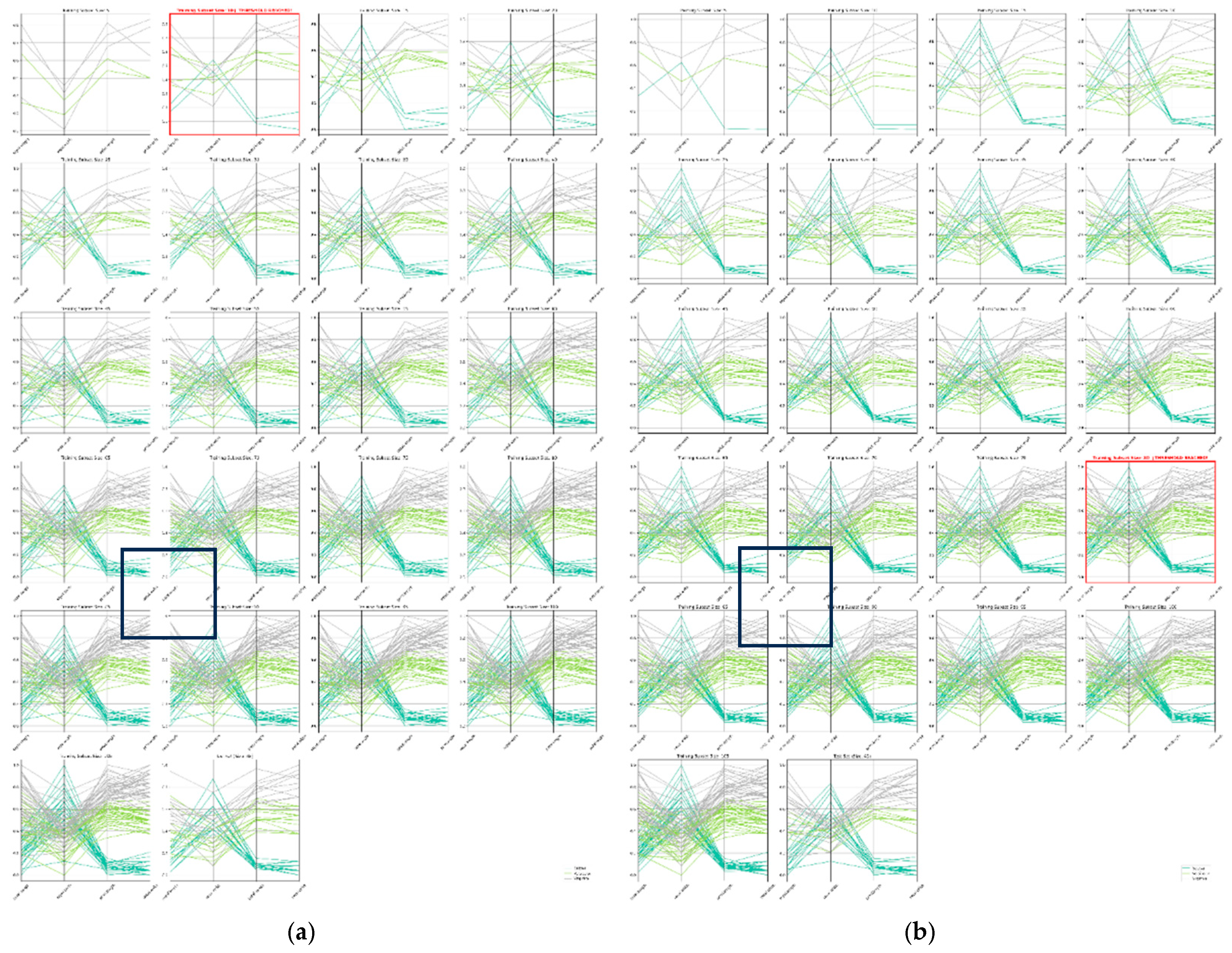
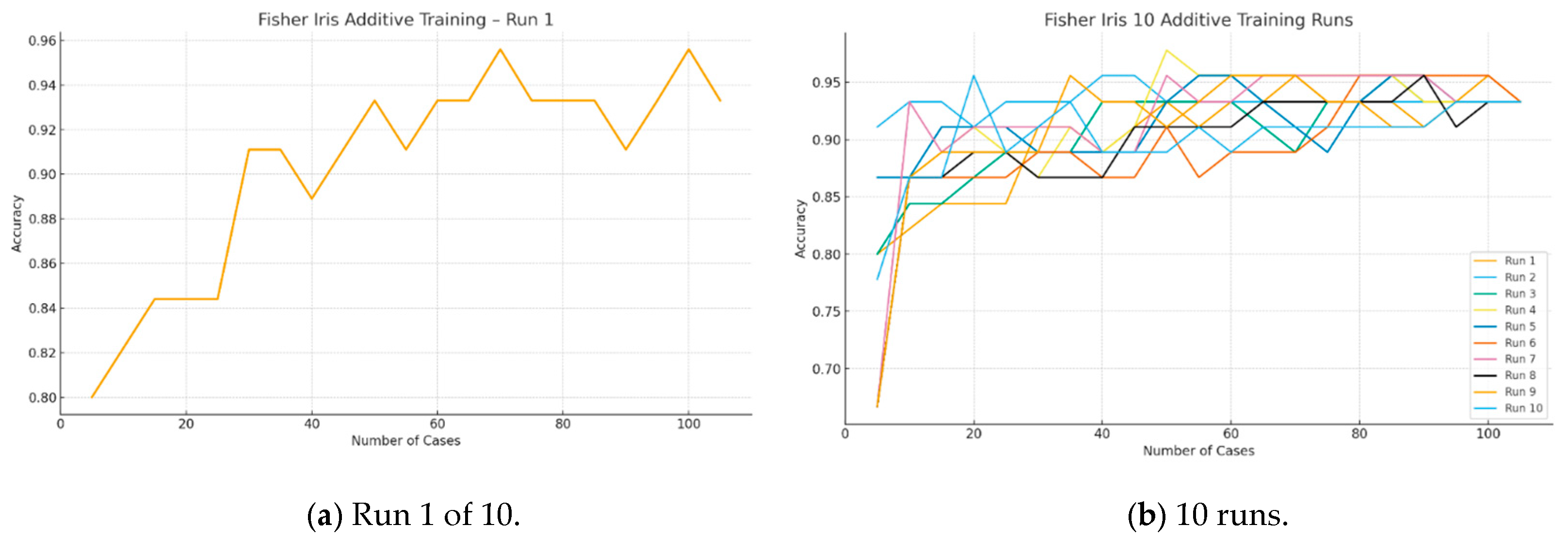
Changes in model accuracy can be measured on both the training and test datasets. A decrease in training accuracy may indicate the addition of more difficult cases, such as noisy cases, cases near class boundaries, or cases located in regions of class overlap. Changes in test accuracy may also indicate a mismatch between the distributions of the training and test data. Section 5 presents examples of non-monotonic accuracy behavior that can be indicative of noise.

Definition 10.

Bounded Noise Reduction (BNR): A positive difference Ac(Small) − Ac(Full) > 0, where Ac(Small) is the accuracy on the Small dataset, indicating that the Full dataset can contain noise cases because their removal increased accuracy. For practical reasons, we often search only for an upper-bound minimal training data subset $S_{UB}$. Computing the exact Model Sureness measure value, or tight bounds on it, can require an exhaustive search involving model evaluations produced by algorithm $A$ over multiple subsets of dataset $S$. The number of such model computations, denoted as $N_{\mathrm{M}\mathrm{C}}$, and the computational cost of each model computation, denoted as $C_{\mathrm{M}\mathrm{C}}$, depend on the algorithm $A$, dataset $S$, and specified accuracy threshold $T$, formally defined below:

Definition 11.

The number of times that algorithm A computes models {M} on subsets of dataset S is denoted as N_MC.

Definition 12.

The complexity of each model computation C_MC by an algorithm A on a subset S_Ri of set S is denoted as C_MC(S_Ri).

Definition 13.

The total complexity of all model computation T_MC by an algorithm A on all selected subsets {S_Ri} of set S is denoted as T_MC(S) and it is a sum of all C_MC(S_Ri):

$$T_{MC}(S)=\sum _{\mathit{i}}^{{\mathit{N}}_{\mathit{M}C}}{C}_{MC }\left(S_{Ri}\right)$$

Definition 14.

The Convergence Rate R is defined where Runs_SUCCESS is the number of runs the model was considered as “sure” and Runs_TOTAL is the total number of runs attempted:

R = Runs_SUCCESS/Runs_TOTAL

While we used the convergence criterion from Definition 14, other or additional criteria may be applied. If convergence fails, exit criteria can be used, as summarized below.

Convergence Criteria:

• Model accuracy on test data. The primary convergence criterion studied in this work is the model accuracy on holdout test data. Testing ML models on unseen data evaluates their ability to generalize to new scenarios. Achieving some comparable test accuracy value (e.g., 95% or 99%) using a reduced training dataset indicates that certain training cases are redundant and not essential for the model performance. The lossless visualization of $n$-dimensional data enables the identification of these redundant cases in the feature space. Evaluations using different holdout test sets may reveal different redundancy patterns, which can be examined through visualization.
• Class-specific failure rate. This criterion is motivated by applications in which the misclassification of certain classes carries a higher risk than others. For example, in medical diagnosis, misclassifying malignant cases may be unacceptable, whereas some errors on benign cases may be tolerated to ensure conservative patient assessment.

Exit Criteria:

• Limiting the number of training iterations. Setting an upper bound on the number of iterations (e.g., 100 or 1000) ensures that computations are completed in a predictable time frame. This also enables fair, apples-to-apples comparisons of different models in terms of computational cost, particularly when evaluating the suitability for deployment on hardware with limited computational resources.
• Limiting model size. Imposing constraints on the model size (e.g., 1 MB or 5 GB) allows control over storage requirements, which is critical for model deployment on any resource-constrained platforms such as IoT devices and embedded systems.

Definition 15.

The Per-Attribute Model Sureness Measure Z is the ratio of the number of unnecessary n-D points S_u: |S_u| = |S| − |S_m| to all points in set S per attribute. Let |D| be the number of attributes in the data D:

Z = (|S_u|/|S|)/|D|

A hypercube is the generalization of the square with the center in point a and side length 2r, where r is a radius of the circle centered in point a.

Definition 16.

The hypercube with the center n-D point a and side length 2r is a set of n-D points {w}, w = (w₁, w₂, …, w_n) such that |a_i − w_i| ≤ r for all i∈ {1, 2,…, n}.

The hyper-rectangle (hyperblock) is a generalization of the rectangle with the center at point a and sides length 2r_i.

Definition 17.

The hyperblock (HB) with the center n-D point a and side length 2r_i is a set of n-D points {w}, w = (w₁, w₂, …, w_n) such that |a_i − w_i| ≤ r_i for all i∈ {1, 2,…, n}.

Definition 18.

The hyperblock algorithm is an ML algorithm that produces on training dataset D a set of hyperblocks HB_ik such that if point a∈ HB_km then a∈ Class k.

Definition 19.

The total number HBs that a hyperblock algorithm A generates will be called the HB algorithm HB complexity of algorithm A.

The HB complexity criterion can be computed for smaller datasets from BAP and similar algorithms. A lower HB complexity (fewer HBs) enables simpler visualization. A representative data subset S intuitively predicts independent test set classes of each case. The formal concept of Model Sureness captures it as follows: Let V = MS (D, W, S, T, A), where V is the value of the Model Sureness measure MS for training data D, test data W, smaller training data subset S, accuracy threshold T (e.g., 0.95), and ML algorithm A. The Model Sureness metric yields value V as a sureness measure of the model M, built by algorithm A, on data D, evaluated on test data W.

Consistent with this paper’s goal, a representative subset S should allow an accurate class prediction for each test case. The formal concept of Model Sureness captures it as follows: Let V = MS (D, W, S, T, A), where V is the value of the Model Sureness measure MS for training data D, test data W, smaller training data subset S, accuracy threshold T (e.g., 0.95), and ML algorithm A. The Model Sureness metric yields value V as a sureness measure of the model M, built by algorithm A, on data D, evaluated on test data W.

The values V act as a measure of representativeness of subset S for A, D, and W. Similarly, set C complements S in D, C = D\S. In addition, values V can measure the redundancy of subset C for D and W. Thus, V measures the representativeness of subset S, and the redundancy of subset C, in addition to being a sureness measure of model M.

These definitions are complementary, not circular. This is because the same value V characterizes different components involved in the Model Sureness measure without introducing other formal definitions. They clarify the role of different components involved in the MS measure. However, the major benefit from presenting them comes from a potential increase in user trust of the model M. Similarly, dot product x⋅y = cos(Q) = 0 defines orthogonality as a property of unit vectors x and y. It also allows us to state that the angle Q between vectors x and y is 90° and cos(Q) = 0.

4.3. Algorithms

Algorithms to compute the Model Sureness measure are executed repeatedly to analyze different training subset selections. In the experiments here, an accuracy threshold of 95% is used. This is also the default setting in the software developed [Supplementary Materials] and is a user-defined parameter that can be adjusted to different tasks. Users should be familiar with the accuracy achieved when training on the full dataset to inform the threshold value. Otherwise, preliminary experiments can be conducted to determine an appropriate accuracy level.

The default number of iterations in the developed software is set at 100; however, this parameter is adjustable. In our experiments, 100 iterations were sufficient to obtain an accurate Model Sureness measure on different datasets. The step size depends strongly on the size of the dataset. In our experiments, using approximately 1% data as the initial step size proved to be a reasonable starting point and was subsequently adjusted based on analysis of the results. Below are the algorithms to compute Model Sureness.

• Generalized Data Search (GDS) Algorithm: This is the generalized single-split case that is characterized by the triplet of the following:

<B_DIR, C, I_MAX>

Here, C is a user-selected criterion that the model is retrained on modified data until achieving. It is represented as a Boolean function such as model accuracy > 0.95.

• Multi-Split Generalized Data Search (MSGDS) Algorithm: This is the generalized multi-split case characterized by the quartet of

<B_DIR, C, I_MAX, S, P>

with two additional parameters of S for split percentage (0 < S < 1), where the test subset percentage is the complement 1 − S value, and P is the number of splits to test.

C is a user-selected criterion which the model is built towards achieving. Note, the number of splits trained should be at least up to a number where the resultant Model Sureness ratios barely change with added splits tested.

• Minimal Dataset Search (MDS) Algorithm: It is characterized by a triplet of the following:

<B_DIR, T, I_MAX>

Here, B_DIR is a computation direction indicator bit. B_DIR = 0 if the MDS algorithm starts from the full set of n-D points S and excludes some n-D points from S. Bit B_DIR = 0 if the MDS algorithm starts from some subset of set S and includes more n-D points from set S. The accuracy threshold T is some numerical percentage value 0 to 1, e.g., 0.95 for 95%. A predefined max number of iterations to produce subsets is denoted as I_MAX. This algorithm (1) reads the triple <B_DIR, T, I_MAX>, and (2) updates and tests the training dataset with the IMDS, EMDS, and AHSG algorithms described below.

• Multi-split Minimal Dataset Search (MSMDS) Algorithm: For data that are not split previously into training and test subsets, the user can specify the split number and percentage. Then, the MDS algorithm is run a split number of times over percentage-sized splits. This gives two additional parameters of S for the split percentage (0 < S < 1), where the test subset percentage is the complement 1—S value, and P is the number of splits to test. This is characterized by the quartet of the following:

<B_DIR, T, I_MAX, S, P>

• Inclusion Minimal Dataset Search (IMDS) Algorithm: This iteratively adds a fixed percentage of n-D points from the initial dataset S to the learnt subset S_i, trains a selected ML classifier A, and evaluates accuracy on all known separate test data S_ev, iterating until all data are added and assessed to reach threshold T, e.g., 95% test accuracy.
• Exclusion Minimal Dataset Search (EMDS) Algorithm: Contrasting with the Inclusion Minimal Dataset Search, this algorithm starts on the entire training dataset S and removes data iteratively, retraining an ML algorithm to assess reaching threshold T.
• Additive Hyperblock Grower (AHG) Algorithm: This iteratively adds data subsets to the training data, builds hyperblocks (hyperrectangles) on the data using the IMHyper algorithm [85], and then tests the class purity per hyperblock on each data subset added.

The initial or final dataset size depends on the minimum cases needed for training, defining how many cases are added or remain after removal. Section 4.4 discusses scaling and runtime, while Section 4.5 covers computational complexity.

4.4. Computational Complexity

Different ML algorithms have widely different computational complexities. Thus, the scaling behavior of the Model Sureness computation depends heavily on the complexity of the selected ML algorithm, the number of runs $t$, and the iteration step size $m$, while other parameters may also influence the computation. In simplified terms, an upper bound on the computational complexity can be expressed as $t\cdot k\cdot C\left(A\right)$, where the term $C\left(A\right)$ denotes the complexity of running the selected ML algorithm $A$ on the full dataset $S$, $k={\displaystyle \frac{\mathrm{TOTAL}\_\mathrm{CASES}}{m}}$, $m$ is the number of cases added or removed at each iteration step, and $t$ is the number of times algorithm $A$ is executed for a given pair $⟨S,m⟩$.

Below, we analyze the computational complexity of the Multi-Split Minimal Dataset Search (MSMDS) algorithm. For the Minimal Dataset Search (MDS) algorithm alone, split-related terms are omitted from the complexity calculations. The MDS algorithm’s complexity matches MSMDS’s, except without the split-number parameter as a scalar multiplier $t$.

Parameters of Complexity Estimates:

• $N$—total number of cases in the dataset;
• $d$—dimensionality of the data;
• $m$—step size (number of cases added or removed per iteration);
• $N/m$—number of iterations for a given data split;
• $sp\%$—training split percentage; for example, $sp\%=70$ indicates that 70% of the $N$ cases are used for training and $1-sp\%=30\%$ are used for the testing;
• $t$—number of different train–test splits;
• $q$—number of training cases used in a given iteration;
• $\mathrm{T}\mathrm{r}(q,d)$—time required to train the model at a given iteration using $q$ cases in $d$-dimensional space;
• $\mathrm{T}\mathrm{r}(N,d)$—an upper bound on $\mathrm{T}\mathrm{r}(q,d)$;
• $\mathrm{T}\mathrm{t}\left(\right(1-sp\%)\cdot N,d)$—time required to test the model on the test dataset;
• $sp\%\cdot N$—number of training cases in a given split.

In these terms, the total upper bound on the computational complexity is as follows:

$$\mathrm{T}\mathrm{o}\mathrm{t}=t\cdot ({\displaystyle \frac{N}{m}})[\mathrm{T}\mathrm{r}(N,d)+\mathrm{T}\mathrm{r}((1-sp\%)\cdot N,d)]$$

(1)

Assume that $\mathrm{T}\mathrm{r}(N,d)+\mathrm{T}\mathrm{r}\left(\right(1-sp\%)\cdot N,d)$ is upper-bounded by constant $C$. Thus, a simplified complexity upper bound is $t\cdot (N/m)\cdot C$. If $t$ and $N$ are comparable, the resultant algorithmic complexity is quadratic with respect to these parameters. When $t$, $m$, and $C$ are treated as constants, the simplified expression $t\cdot (N/m)\cdot C$ indicates a linear algorithmic complexity $O\left(N\right)$ with respect to the number of cases $N$. In contrast, a brute-force exploration of all subsets of $N$ cases yields an exponential complexity of $O\left(2^N\right)$.

For the WBC dataset, which contains 683 cases, a 70%:30% split yields 478 training cases that can be selected from $C\left(\mathrm{683,478}\right)$ possible combinations, which is approximately $5.7\times {10}^{179}$ and is intractable to explore exhaustively. Testing multiple test sets arising from this combinatorial number of training datasets is thus not feasible. Consequently, we used either a fixed test set, as is commonly done for MNIST, or test sets selected ourselves. These limited test sets may miss the worst-case data splits; thus, as part of future work, we propose identifying the worst-case splits using methods such as those described in [6] to obtain a more complete Model Sureness measure.

Formula (1) does not provide a tight upper bound, because training a model on smaller data subsets typically requires less time than training on the full dataset assumed in (1). Another reason that (1) is not a tight bound is that a predefined accuracy threshold $T$ may be reached without executing the ML algorithm $A$ for all ${\displaystyle \frac{N}{m}}$ iterations. Consequently, (1) represents a worst-case estimate. A best-case estimate occurs when the ML algorithm achieves the required accuracy after a single run. In our experiments, reported in the next section, the computation time was reasonable, as demonstrated by the presented results.

4.5. Scaling

To analyze the scaling of the Model Sureness measure computational method, we may consider two algorithms, $A_1$ and $A_2$, with the same Model Sureness measure, for example, 0.8, but where algorithm $A_1$ requires half the computation time of algorithm $A_2$ to compute its Model Sureness measure, because $A_2$ is more complex. Algorithm $A_1$ therefore has an advantage in requiring fewer computational resources to compute its Model Sureness, in enabling additional experiments to identify different smaller subsets, and to explore Model Sureness more broadly. This advantage is particularly important for any algorithms with stochastic components, which can lead to models with varying accuracies across different runs. To account for this output variability, we run such algorithms multiple times and measure both the Model Sureness and its standard deviation.

The following three benchmarks report the actual elapsed computational time for datasets of different sizes. These tests use a linear SVM as the algorithm and measure time scaling across different datasets and values of $m$. All computational time-scaling tests were performed using multithreaded CPU execution on the same Intel 8-core i7-7700 CPU at 3.60 GHz, with 16 threads and 32 GB of RAM, running Debian Linux.

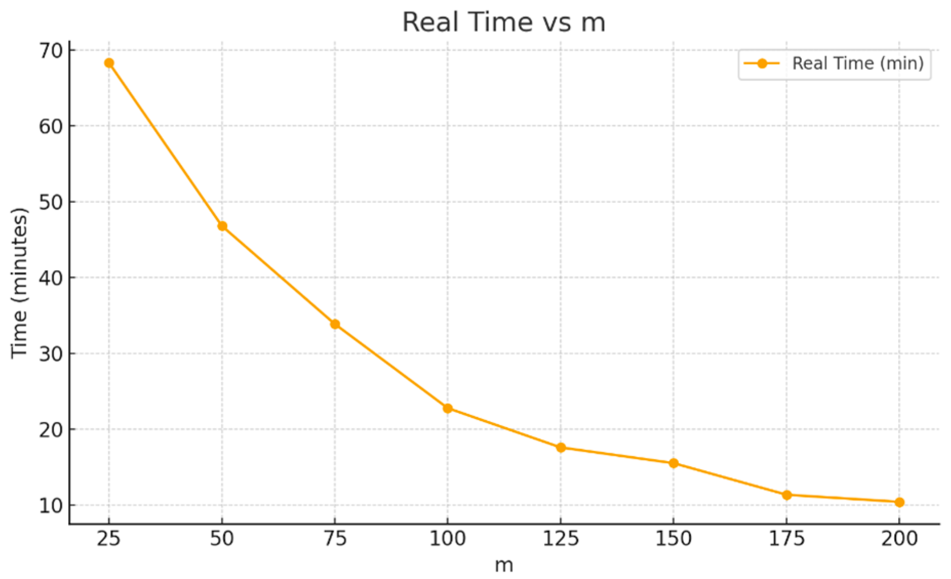
In the first experiment, we used the MNIST dataset, which is pre-split into 60,000 training cases and 10,000 test cases. In this experiment, 10 runs ($t=10$) were conducted for each value of $m$ (ranging from 25 to 200 cases) on the same data split, using BAP in a forward-direction for Model Sureness testing in which $m$ cases are added at each step. The ML algorithm $A$ used was a linear SVM. All tests in this study converged to a model accuracy of 95% or higher on the test data.

Figure 4 shows the results. Using a small step size of $m=25$ cases required approximately 70 min, whereas an eight-times larger step of $m=200$ cases required about 10 min. These times correspond to 10 runs; thus, each individual run took approximately 7 min and 1 min, respectively. Note that, for 60,000 training cases, a step of 25 cases represents only 0.042% of the dataset, and even the larger step of 200 cases corresponds to only 0.33% of the dataset. Therefore, both step sizes are well below 1% of the dataset—this enables a more fine-grained Model Sureness evaluation process.

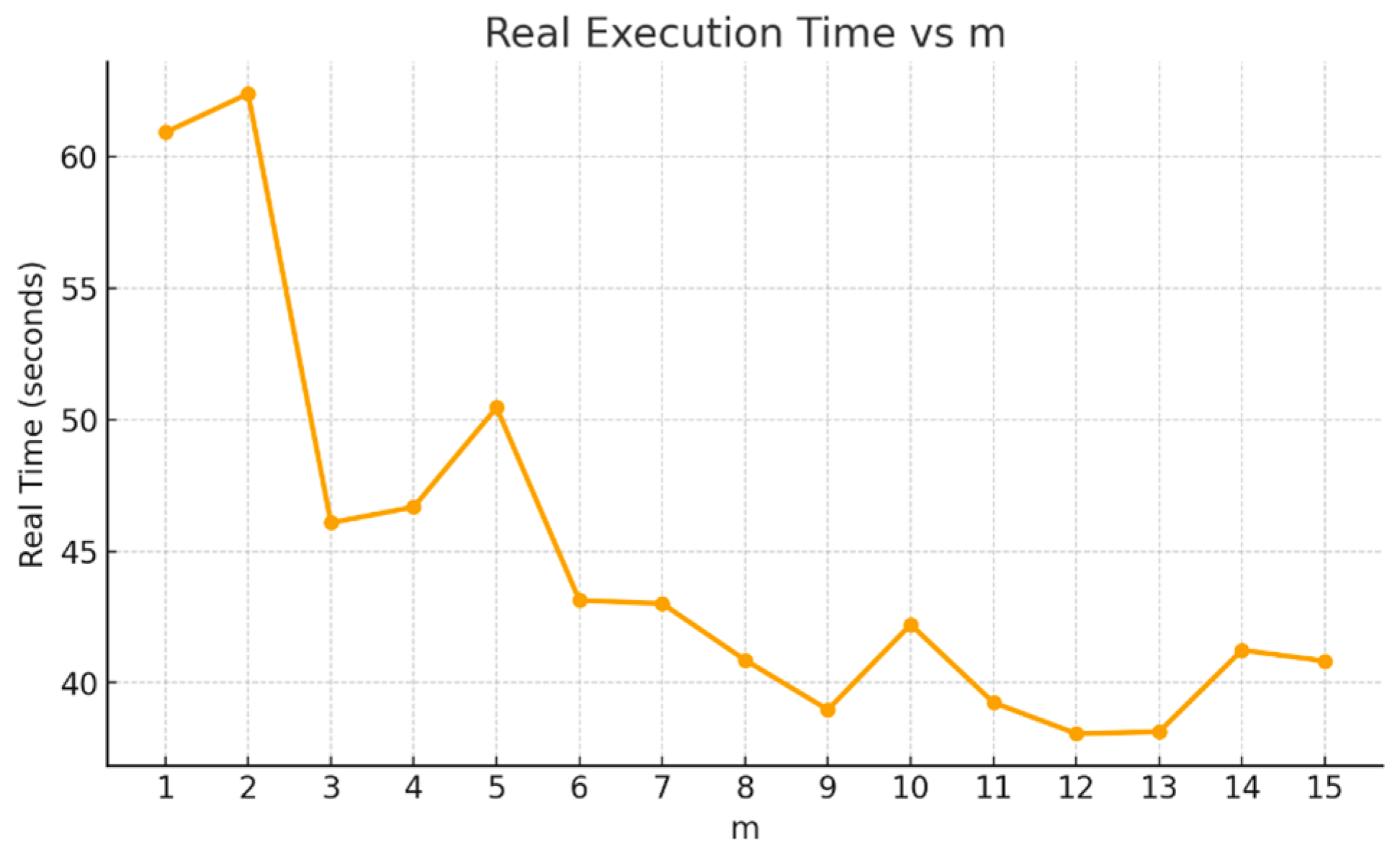
Figure 5 shows the results for the Fisher Iris dataset using a 70%:30% split of the 150 cases into training and test datasets. For a given split, we ran model training 100 times ($t=100$) to build models on the training data with step sizes ranging from a single case to 15 cases per step ($m=1:15$). Thus, for this small dataset, the step size $m$ varies from approximately 1% to 15% of the training dataset. In this experiment, for each split, we performed 100 iterations, each time adding randomly sampled cases to the training data. Since we evaluated 15 different values of $m$, the algorithm was run 100 times for each value of $m$ (e.g., for $m=1$, the algorithm was run 100 times).

Therefore, the entire model-training process was independently executed a total of $15\times 100\times 100=\mathrm{150,000}$ times. Moreover, instead of using only one singular 70%:30% training–test split, we employed 100 randomly generated splits (parameter $sp=100$). This means that the linear SVM algorithm was run a total of $sp\times t=100\times 100=\mathrm{10,000}$ times for each value of $m$. The analysis of the results shown in Figure 5 indicates that the most computationally intensive experiment required only approximately 170 s.

Figure 6 shows the results for the WBC dataset using 70% of the 683 cases for training, with 100 random splits and 100 model-training iterations per split. The step size $m$ varied from 1 to 15 cases, corresponding to approximately 0.15% and 2.2% of the total dataset, respectively. The analysis of the results that is shown in Figure 6 indicates that the most computationally intensive experiment required only about 70 s.

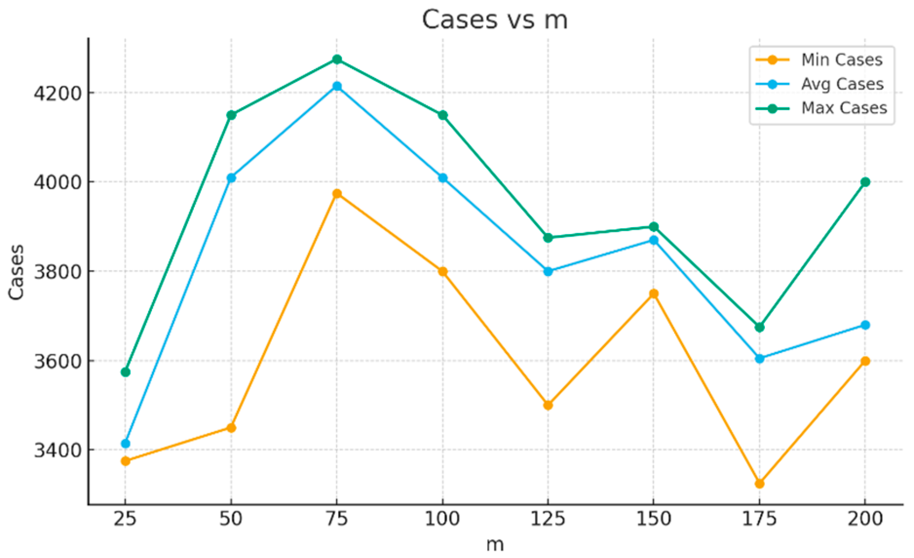
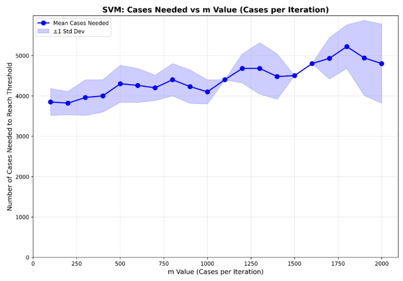
Figure 7 shows, for the MNIST handwritten digits dataset, the number of cases required for each test to converge to the 95% accuracy threshold. The green line represents the maximum number of cases, the blue line represents the average number of cases, and the orange line represents the minimum number of cases across the 10 runs. The average curve is close to the maximum curve, indicating that the average values are representative of most runs and that the maximum does not correspond to particularly unusual cases.

The number of cases on the average curve range from 3400 to 4200, or 5.7–7.0% of the full 60,000-case dataset. The maximum curve ranges from 3600 to 4300 cases, or 6.0–7.2% of the dataset. The minimum curve varies from 3400 to 3600 cases, corresponding to 5.7–6.0% of the data. Thus, although the curves in Figure 7 are not monotonic, the variability for the maximum and average curves remains within approximately 2% of the total training data. The variability is more pronounced for the minimum (orange) curve; however, it is still relatively small, with the maximum value remaining below 4000 cases.

4.6. Pseudocode

This section presents the pseudocode for the Multi-Split Minimal Dataset Search (MSMDS) algorithm in Algorithm 1. The algorithm is implemented in the provided open-source code. The inputs and procedural steps of the MSMDS algorithm are as follows:

Algorithm 1 Multi-Split Minimal Dataset Search

Input: sp%, sp, t, dataset, classifier, direction, threshold T, step m. Example: sp% = 70 (training data fraction, sp = 100 number of different sp%, t = number of runs of each split sp%, dataset = WBC, classifier = ‘SVM-linear’, direction = ‘additive’ (alternative is subtractive)), T = 0.95, m = 5. Algorithm:        1. Loop sp times:        2. training_data, test_data = split dataset to sp% and 1 − sp%       Loop t times:        3. accuracy = 0        4. if direction == ‘subtractive’:               train_subset = training_data        5. else:               train_subset = []        6. While accuracy ≤ T:        7. if action == ‘subtractive’:               if len(train_subset) ≥ m:                             Remove m cases from train_subset               else:                             break //subset not found        8. else:               if len(training_data) ≥ m:                             Move m cases to train_subset from training_data               else if training_data not empty:                             train_subset = training_data               else:                             break //subset not found               Train classifier on train_subset               accuracy = evaluate classifier on test_data               if accuracy ≥ T:                             Save train_subset //subset found

5. Case Studies

This section presents case studies on the Fisher Iris [16], Wisconsin Breast Cancer [16], and MNIST [14] datasets, with the results, analysis, and conclusions.

5.1. Fisher Iris Classification

5.1.1. Computational Experiment

Table 2. SVM linear classifier and MSMDS algorithm on the Fisher Iris data with all three classes of 150 total cases, using a ten-case step, 70%:30% split (105 training cases:45 test cases), and an accuracy threshold of 95%.

Characteristics	Number of SVM Linear Iterations
	10	100	1000
Mean Cases Needed	37.8 ± 22 [15.8, 59.8]	31.6 ± 16.5 [15.1, 48.1]	31.8 ± 18.5 [13.3, 50.3]
Mean Cases Needed %	36% ± 21% [15%, 59%]	30.1% ± 15.7% [14.4, 45.8]	30.3% ± 17.6% [12.7, 47.9]
Min Cases Needed	10	10	10
Min Cases Needed %	9.5%	9.5%	9.5%
Max Cases Needed	90	90	100
Max Cases Needed %	85.7%	85.7%	95.2%
Mean Model Accuracy	0.953 ± 0.035	0.959 ± 0.026	0.961 ± 0.026
Convergence Rate *	9/10 = 90%	93/100 = 93%	919/1000 = 91.9%
Mean Model Sureness measure ratio	1 − 0.36 = 0.64	1 − 0.301 = 0.699	1 − 0.303 = 0.697

* The convergence rate is measured as the ratio of the number of times the model is considered “sure” (under a given accuracy threshold) to the total number of iterations run.

shows the Fisher Iris case study results using a linear SVM with 10, 100, and 1000 iterations. The model reached 95% accuracy using between 9.5% and 95.2% of the training data. With 1000 iterations, the mean data requirement ranges from 12.7% to 47.9% of the training set. Across 10 runs, an average of 37.8 out of 105 training cases (36%) was needed to reach 95% accuracy. The required cases varied widely, from 10 (9.5%) to 90 (85.7%).

These results reveal differences in the subset and case importance, enabling a deeper analysis of the most informative data. For instance, the 10-case minimal subset in Figure 4 can be compared with a less informative 80-case subset. Smaller subsets like this are easier to analyze visually using lossless data visualization (e.g., with Parallel or General Line Coordinates), a topic for future study.

Figure 8 shows a Parallel Coordinates visualization of the identified subset of cases together with the full set of 105 training cases obtained from a 70%:30% train–test split. As shown in Figure 8a, the Setosa class requires only two cases to accurately represent the shape of the data in $n$-D space. In contrast, the Versicolor and Virginica classes each require four cases to adequately describe their structure for a linear SVM classifier model.

Notably, Versicolor and Virginica are more alike in shape than Setosa, explaining the higher number of required cases. More similar classes need more examples to capture subtle distinguishing differences. Across 100 runs, nearly identical results show that fewer than half the training cases suffice for an accurate classification with the linear SVM. The step size was 10 cases, the accuracy threshold 0.95, and data split 70:30 for training and testing.

Figure 9 presents Parallel Coordinates visualizations of progressively increasing training subsets used in these experiments, allowing a visual analysis of the iterative growth of the training data until the accuracy threshold is reached. Initially, each class is visually represented by only a few cases. Over successive iterations, as five additional cases are added at each step, the feature space becomes increasingly dense, eventually producing a relatively uniform distribution of cases that delineates the class boundaries. The test data are visualized in the final Parallel Coordinates plot for comparison.

This process follows an additive strategy, beginning with a small training dataset and incrementally adding cases at each iteration while monitoring whether the 95% test data accuracy threshold is satisfied. Figure 9a shows that the 95% accuracy threshold is reached quickly in the second iteration, whereas, in Figure 9b, it is reached much later due to a higher accuracy threshold of 99%. Figure 9 also illustrates the backward process: starting from full data, (a) takes 16 iterations to minimal dataset; backward from a smaller subset, (b) reaches it faster, assuming the same selections.

Figure 10 shows 10 runs where the Fisher Iris training sets grow by five cases per step using a 70:30 train–test split. Models are trained on independently growing subsets for each iteration and evaluated on initially fixed test data. A key advantage of Figure 10 is that the staggered non-monotonic behavior in the test accuracy of consecutive training subsets can indicate the addition of difficult cases, such as noisy or ambiguous cases. This also shows 91% accuracy with 35 cases, dropping to 89% when it increased to 40 cases. This suggests these five cases challenge the classifier. If a noise analysis confirms it, remove them from training; otherwise, add cases to restore accuracy. The visualization of these specific cases can support this diagnostic analysis. To enable this evaluation, a pre-split test dataset is first defined and used for analysis. Due to the combinatorial explosion of possible train–test splits, it is not feasible to explore all configurations. Thus, in some experiments, data are split prior to exploration with some specific splits examined in detail.

Table 3. Results of measuring Model Sureness on Fisher Iris data with all three classes for 150 total cases, using LDA algorithm, and 70:30 split. with the MSMDS algorithm adding 10 cases from 70:30 split to threshold of 95%.

Characteristics	Number of LDA Iterations
	10	100	1000
Mean Cases Needed	19 ± 5.4 [13.6, 24.4]	21.3 ± 14.3 [7, 35.6]	21.1 ± 14.5 [6.6, 35.6]
Mean Cases Needed %	18.1% ± 5.1% [13%, 23.2%]	20.3% ± 13.6% [6.7%, 33.9%]	20.1% ± 13.8% [6.3%, 33.9%]
Min Cases Needed	10	10	10
Min Cases Needed %	9.5%	9.5%	9.5%
Max Cases Needed	30	100	100
Max Cases Needed %	28.6%	95.2%	95.2%
Mean Model Accuracy	0.980 ± 0.018	0.977 ± 0.021	0.977 ± 0.02
Convergence Rate	10/10 = 100%	99/100 = 99%	981/1000 = 98.1%
Mean Model Sureness measure ratio	1 − 0.181 = 0.819	1 − 0.203 = 0.797	1 − 0.201 = 0.799

shows Linear Discriminant Analysis (LDA) classifier results for 10, 100, and 1000 iterations. The Iris dataset, containing all three classes and totaling 150 cases, was split 70%:30% into training and test sets, resulting in 105 training cases. These results show LDA requires 9.5–95.2% of data, similar to linear SVM, as both are linear classifiers.

Since Model Sureness applies to any ML algorithm, we next study an interpretable classifier using hyperblocks (HBs), and then a black-box convolutional neural network (CNN) model. This enables a comparison of three distinct ML algorithms using the same metric and provides a new way to evaluate the quality of HBs, using the algorithm from [89] to generate interpretable HB (hyper-rectangles) classification models. This approach tests the HB structures each iteration, assessing the geometric model robustness.

In each experiment iteration of

Table 4. Results of evaluating the Fisher Iris with Versicolor and Virginica classes by the Additive Hyperblock Grower (AHG) algorithm; the HBs have been grown with IMHyper algorithm [89].

Characteristics	Number of AHG Iterations
	10	100	1000
Mean Cases Needed	76.2 ± 14.3 [61.9, 90.5]	75 ± 17.4 [57.6, 92.4]	74.4 ± 19.9 [54.5, 94.3]
Mean Cases Needed %	72.57% ± 13.59% [58.98%, 86.16%]	71.43% ± 16.54% [54.89%, 87.97%]	70.89% ± 18.95% [51.94%, 89.84%]
Min Cases Needed	59	40	22
Min Cases Needed %	56.19%	38.1%	20.95%
Max Cases Needed	98	104	105
Max Cases Needed %	93.33%	99.05%	100%
Mean Model Accuracy	0.9556	0.9586	0.8648
Convergence Rate	5/10 = 0.5 = 50%	37/100 = 0.37 = 37%	295/1000 = 0.295 = 29.5%
Mean Hyperblocks	3.4 ± 0.5	3.8 ± 0.9	3.8 ± 0.9
Min Hyperblocks	3	3	3
Max Hyperblocks	4	6	8
Mean Model Sureness measure ratio	1 − 0.7257 = 0.2743	1 − 0.7143 = 0.2857	1 − 0.7089 = 0.2911

, five cases were added to the training set, and the HBs expanded to include them. The resulting models were then evaluated on the test data to detect any introduced case misclassifications. For the Fisher Iris dataset, no misclassifications were observed when constructing HBs using 100 training cases for the two classes Versicolor and Virginica. This results from the IMHyper algorithm [90], which prioritizes a pure HB formation.

This additive procedure is more fine-grained and results in tighter HB bounds. This is evident when comparing it to applying the IMHyper algorithm directly to the full training dataset of 100 cases without incremental growth where, in that case, the algorithm produced four HBs rather than two.

To find improved IMHyper parameters (purity/impurity thresholds and number of cases added per iteration), a grid search is conducted over potential parameter values:

• Training percentages: [0.7] (fixed);
• Random seeds (splits): [42, 123, 456, 789, 999];
• Accuracy threshold: 0.95.

Parameter ranges:

• Case(s) added per step: [1, 2, 3, 5, 10];
• Hyperblock purity-threshold: [0.8, 0.85, 0.9, 0.95, 1.0];
• Hyperblock impurity-threshold: [0.05, 0.1, 0.15, 0.2, 0.25].

This has 625 parameter combinations. This was run in parallel on an AMD Ryzen 9 5900X (12-core CPU @ 3.70 GHz with 24 threads and 64 GB RAM) running Windows 11.

A grid search identified the optimal parameters for IMHyper with AHG algorithms to build an HB model for the Table 4 results. The selected parameters are as follows:

• Case(s) added per step: 1;
• Hyperblock Purity threshold: 0.8;
• Hyperblock Impurity threshold: 0.7;
• Train percentage: 0.7;
• Random seed: 999 (initial seed used, incrementally increased per iteration.).

Each individual hyperblock (HB) is a simple geometric model; however, the total number of HBs required to cover the training data can be large, and some HBs may be redundant. One algorithm described in [89] addresses this issue by analyzing and reducing the number of HBs. The Minimal Dataset Search (MDS) algorithm identified a smaller training subset that is sufficient for achieving the required test data accuracy of 95%, and both the MDS and MSMDS algorithms were able to find such reduced datasets efficiently.

Using these reduced datasets, it is possible to construct a simpler set of HBs than those generated from the full training data. Indeed, when the IMHyper algorithm [89] was applied directly to the full training dataset of 100 cases, without starting from a small subset and incrementally growing it, this produced four hyperblocks rather than two. This demonstrates that building a hyperblock-based model by iteratively adding cases can yield a more compact and parsimonious model.

5.1.2. Interactive Visual Experiment

A Computational Interactive Visual Learning (CIVL) process that is conducted with a human-in-the-loop [9] is applicable for identifying smaller training datasets. Below, we outline this approach and illustrate it with an example, a Divide-and-Classify process that separates training cases into simple and complex subsets, which are then each classified independently through computational analysis and data visualization using lossless data visualization spaces such as Parallel Coordinates or other General Line Coordinates.

Simple cases lie in pure regions containing only one class, while complex cases appear in overlap regions where multiple classes coexist. Because the pure training data cases are already classified with 100% accuracy, we can test whether the accuracy of test cases that fall within the same pure regions identified in the training data is acceptable. If this condition is met, we can select a subset of training cases from pure regions to maintain high accuracy, keeping overlap cases in the dataset. This yields a smaller training set when overlap cases are few, as shown in Figure 2.

Figure 11a shows a minimal training set sufficient for linear threshold classifiers on the Fisher Iris dataset [16]. These data contain two pure regions: (1) the area above the upper orange line and (2) the area below the lower orange line. Case b, located above the upper orange line, is the lowest case in the upper pure region. Correspondingly, case a is the highest case in the lower pure region. Cases c and d, which lie adjacent to these, represent the bottom and top cases of the overlap region, respectively.

Cases a and b are sufficient to classify all pure training cases. If they also correctly classify the test cases that fall within these regions, then they are sufficient to classify those cases as well. Keeping in the training data all cases between cases a and b yields a reduced training set of 10 cases out of the total 100 cases from these two classes. A linear classifier using the orange threshold line misclassifies three of the ten cases, achieving 70% accuracy. If 10 cases were randomly selected as the smallest training dataset, the set of cases between a and b could constitute one such selection. This would represent the worst possible split with a 10-case training subset for a linear classifier model, since it fully covers the overlap region between the two classes, again yielding only 70% accuracy.

Given a desired classification accuracy of 95% on both training and test datasets, this 10-case training subset is insufficient, and additional cases are required. By adding cases located below a and above b, which are correctly classified using the same threshold, the training set can be expanded. With 60 test cases and the same three misclassifications, the accuracy is 95% (57/60); the 40 training cases reach 100%.

An opposite extreme (best-case test scenario) occurs when no overlap cases between a and b are included in the test data. In this case, all test cases are classified with 100% accuracy using the same threshold. This setup yields 90 cases, leaving 10 overlap cases in training, which reach only 70% accuracy. To reach 95% training accuracy, the set must be expanded to 60 cases, 20 more than the 40 cases needed in the first extreme scenario.

These results are consistent with the purely computational BAP results in Table 1 for the same Fisher Iris dataset using a linear SVM. The mean plus standard deviation of cases required in Table 1 is about 60 cases. The maximum percentage of cases in Table 1 is from 85.7–95.2%, while the result presented above corresponds to 60% of the cases.

Figure 11b shows two Fisher Iris classes in Parallel Coordinates, with identified boundaries around pure regions. This visualization lets users interactively find smaller sufficient training sets. For the pure region above the upper black line, one representative case is sufficient. Similarly, for the pure region below the lower black line, only one representative case is sufficient. Determining the optimal accuracy threshold requires several cases from the overlap region to define a sufficient reduced training set.

The next experiment with Visual Knowledge Discovery on the Fisher Iris data uses a hyperblock classifier algorithm [91,92] that produces logical rules such as the following:

R: if a₁₁ ≤ x₁ ≤ a₁₂ & a₂₁ ≤ x₂ ≤ a₂₂ & … & a_n1 ≤ x_n ≤ a_n2 then x ∈ Class C_k

If each attribute x_i of case x is in a specific interval a_i1 ≤ x_i ≤ a_i2, then case x belongs to class C_k. In Parallel Coordinates, such rules are visualized as a low strip a₁ = (a₁₁, a₂₁, a_n1) and high strip a₂ = (a₁₂, a₂₂, a_n2) of case bounds, respectively. If bounds a₁ and a₂ are actual training cases, then we have the smallest sufficient training data subset with only two cases for class C_k. Alternatively, we need the smallest set of cases that have all values a_ij covered. In the worst case, we would need 2n such cases if each case has only one a_ij value. If rule R has a simple written form with a single attribute x_i (R: if a_i1 ≤ x_i ≤ a_i2 then x ∈ Class C_k), then only two cases are needed to discover this rule with respective values a_i1 and a_i2. For discovering the simplest rule, only a single case x is needed with a_i1 = x_i to discover this rule:

R: if a_i1 ≤ x_i then x Î Class C_k

For the two Iris classes (Virginica and Versicolor), 14 simple rules, each using 2 cases, totaling 28, were visually identified to cover all 100 cases. These sequentially dependent rules form a tree structure [9] and the generation sequence is shown in Figure 12, updated from [9]. Red and green coordinate segments in this figure denote intervals a_i1 ≤ x_i ≤ a_i2. The majority of cases in intervals belong to the red or green class, respectively. In this study, the threshold for the majority is 98% (2 cases out 100 cases misclassified). Figure 12a shows 7 intervals (4 red and 3 green) requiring 14 cases to represent them. These 14 cases classified 74 cases (74%). Similarly, Figure 12b–e show the intervals produced in the next iterations.

5.2. Wisconsin Breast Cancer Diagnosis

This case study follows the same approach as Section 5.1 but uses a data step size of 20 cases. The best WBC results in

Table 5. Results of SVM experiments on cancer data with data step size of 20 cases added each training iteration, with 70%:30% split (478 train cases and 205 test cases), and an accuracy threshold of 95%.

Characteristics	Number of Iterations of SVM Linear
	10	100
Mean Cases Needed	20	21 ± 5.2
Mean Cases Needed %	4.2% [4.2%, 4.2%]	4.4% ± 1.1% [3.3%, 5.5%]
Min Cases Needed	20	20
Min Cases Needed %	4.2%	4.2%
Max Cases Needed	20	60
Max Cases Needed %	4.2%	12.6%
Mean Model Accuracy	0.975 ± 0.01 [0.965, 0.985]	0.969 ± 0.011 [0.958, 0.98]
Convergence Rate	10/10 = 100%	99/100 = 99%
Mean Model Sureness measure ratio	1 − 0.042 = 0.958	1 − 0.044 = 0.956

reach 98.5%, and this study targets at least 95% accuracy. This is slightly lower than the best reported result in the prior literature on 10-fold cross-validation, not a 70:30% split, which achieved accuracies of 97.01–100% [90,93].

Table 6. Results of LDA experiments on cancer data with data step size of 20 cases added each training iteration, with 70%:30% split (478 train cases and 205 test cases), and an accuracy threshold of 95%.

Characteristics	Number of Iterations of LDA
	10	100
Mean Cases Needed	55 ± 31.4	37 ± 20.3
Mean Cases Needed %	11.5% ± 6.6% [7.4%, 15.6%]	7.9% ± 4.2% [7.1%, 8.8%]
Min Cases Needed	10	10
Min Cases Needed %	2.1%	2.1%
Max Cases Needed	130	120
Max Cases Needed %	27.2%	25.1%
Mean Model Accuracy	0.954 ± 0.004 [0.952, 0.957]	0.96 ± 0.008 [0.959, 0.962]
Convergence Rate	10/10 = 100%	100/100 = 100%
Mean Model Sureness measure ratio	1 − 0.115 = 0.885	1 − 0.079 = 0.921

shows the results of using 10 and 100 runs of LDA using case increments of 10 cases added. The cases needed for LDA are substantially more than those for SVM linear with similar Model Sureness measure scores for both and a slightly more reliable convergence rate for LDA.

Figure 13 shows a plot of 10 runs additively building the WBC training data in 10 case increments for one fixed split of 70%:30% train:test data. Then, models are built on the incrementing subsets of training data and then evaluated on the pre-selected test data. The benefit of Figure 13 is that it shows non-monotonic behavior on the test data accuracy for consecutive data subsets which can suggest cases added were difficult cases such as noise cases.

5.3. MNIST Digit Handwritten Digit Recognition

This case study on the MNIST handwritten digits dataset applies a $k$-NN classifier after the dimensionality reduction of a three-pixel edge-crop and average pooling with a $2\times 2$ kernel, and stride of 2. Then, 100 cases are added iteratively to the training set, and the k-NN performance is evaluated on the test set. The accuracy converges to 97.2% in all runs.

Table 7. MNIST results using k-NN, adding 100 cases per iteration until 95% accuracy.

	Number of k-NN Iterations
Characteristics	10	100
Mean Cases Needed	9600	9600
Mean Cases Needed %	16%	16%
Min Cases Needed	9600	9600
Min Cases Needed %	16%	16%
Max Cases Needed	9600	9600
Max Cases Needed %	16%	16%
Mean Model Accuracy	0.972	0.972
Convergence Rate	10/10 = 10%	100/100 = 100%
Mean Model Sureness measure ratio	1 − 0.16 = 0.84	1 − 0.16 = 0.84

and

Table 8. Case-per-class distribution for smaller MNIST training sets from k-NN (k = 3) achieving 97.2% accuracy.

Cases Per Class Label	Case Count	Percentage
0	954	9.94%
1	1088	11.33%
2	946	9.85%
3	985	10.26%
4	953	9.93%
5	834	8.69%
6	976	10.17%
7	1029	10.72%
8	899	9.36%
9	936	9.75%

, and Figure 14 summarize the results. Table 7 shows 16% of the data (9600 of 60,000 cases) achieves 97.2% test accuracy. This shows the stability of k-NN on the MNIST dataset.

Table 8 shows a balanced digit distribution, about 1000 cases per class, matching the full MNIST dataset distribution.

Figure 14 shows a Parallel Coordinates plot of the 9600-case subset achieving 95% test accuracy with $k$-NN ($k=3$), after reducing from 784 to 121 dimensions. Figure 14a–j show the individual digits; 14k shows all of them together.

Figure 15 shows trends in the behavior of different digits as reflected in the width, density, and prevalence of peaks, which correspond to rows of pixels in the MNIST image data. Despite the significant occlusion when all the digits are shown together in Figure 14k, their differences remain visually evident.

This case study shows that a much smaller MNIST subset suffices for the task. This is the case even after the application of data dimensionality reduction, while still achieving an over 95% test data accuracy with a $k$-NN classifier using $k=3$ and the Euclidean distance metric. This demonstrates that the k-NN algorithm exhibits a high Model Sureness on the MNIST dataset for $k=3$ and the distance metric.

Figure 16 shows that the results of 10 runs in which the MNIST training data are additively built in increments of 1000 cases for a single 70%:30% train–test split, with an evaluation performed at each step on the test data. A key advantage of Figure 16 is that non-monotonic behavior in test accuracy across consecutive training subsets can indicate the inclusion of difficult cases, such as noisy cases.

Figure 17 shows how many training cases were needed to reach 95% test accuracy on the MNIST test set in 10 runs with varying batch sizes per iteration. The results indicate that with a smaller step size (250 cases), approximately 4000 training cases are required on average to reach the threshold. In contrast, with a larger step size (2000 cases), only about 5000 training cases are required, with a high variability ranging around 4000–6000 cases.

Therefore, these MNIST data contain little noise with substantial redundancy. The low level of noise may be a consequence of the dimensionality reduction process, which can be further validated through additional experiments using different data dimensionality reduction parameters to assess the stability of the applied transformation. The proposed Model Sureness measure can also be extended from dependence solely on the number of cases $N$ to include the variation in data dimensionality $d$. In this way, Model Sureness can be evaluated for data size pairs $(N,d)$.

Figure 18 and Figure 19 show PCA and t-SNE visualizations of the Model Sureness analysis on data reduced to 121 dimensions, illustrating that, despite being lossy methods, they still capture similarities between the 9600-case subset and the full dataset. At the same time, the differences between the visualizations of the subset and the full dataset are evident. These differences may arise either from genuine distinctions between the datasets or from distortions that are introduced by the lossy transformations performed by PCA and t-SNE.

Data visualizations in Figure 18 allow for the visual verification of cluster shape and location consistency between the full and reduced datasets. This consistency is essential in order to preserve the behavior of the k-NN classifier across both datasets.

Figure 19 shows the class centroids are highly similar under PCA and t-SNE before and after data reduction, confirming the data subset stability. These centroid comparisons are used as a visual mechanism to confirm or refute potential model drift [87].

Below, we present the results of the experiments using a convolutional neural network (CNN) on the same MNIST dataset. We trained a CNN model [92] on all 60,000 training cases for 50 epochs. Using the same architecture and hyperparameters, we obtained the test accuracies on all 10,000 test cases reported in

Table 9. CNN accuracy with and without dimensional reduction on the full 60,000-case MNIST training set.

Training Data (All 60,000 Training MNIST Cases)	Accuracy on All Test Data (10,000 Cases)
Data: 28 × 28 images (784-dimensional)	99.57%
Data: 11 × 11 images (121-dimensional; obtained by cropping image edges by 3 pixels and applying average pooling with a 2 × 2 kernel and stride 2)	99.34%

.

A testing accuracy loss of only 0.23% after dimensionality reduction allows for a more efficient Model Sureness exploration in the reduced feature space. We conducted active learning using parallelized processing to identify training data subsets that achieve 95% accuracy on the same 10,000 test cases. In this process, 100 cases are added at each iteration, the model is trained and evaluated on all 10,000 test cases, and the procedure is repeated until the 95% accuracy threshold is reached. The results are summarized in

Table 10. Results of model accuracy given various reduced training data subsets.

Accuracy on All Test Data	Sample Count
95.36%	2800
96.25%	3200
95.20%	2500
95.93%	2700
96.79%	2800

.

This yields the best model across five trials, using only 2500 training case, with only 4.17% of the 60,000 available. Figure 8 shows a Parallel Coordinates data visualization of these approximately 2800 selected cases. Figure 20 presents the Parallel Coordinates visualization of the highest-accuracy training data subset result from a run that produced 2800 training cases and achieved 95.36% accuracy.

Comparing 9600 vs. 60,000 MNIST training cases shows about a 90% reduction in computation time. These savings are crucial for later iterations in MNIST and other large datasets. While the model training time is highly dependent on algorithm-specific hyperparameters, for example, the Random Forest training time depends on the number of estimators, whereas the k-NN classifier used in our case studies requires only 0.01 s to compute a model using 9600 training cases after dimensionality reduction. The time required to compute the model using all 60,000 of the training cases is reported in

Table 11. Results show training times (in seconds) with and without dimensional reduction for 9600 and 60,000 training cases, measured on an Apple Mac M3 (8-core, 16 GB RAM).

Training Data Cases	Training Time without Dimensional Reduction	Dimensional Reduction Time	Training Time with Dimensional Reduction
9600	1.31	2.48	0.01
60,000	1.23	15.75	0.03

.

Total time to prepare the data and train the model with dimensionality reduction was $2.48+0.01=2.49$ s for 9600 and $15.75+0.03=15.78$ s for 60,000 training cases.

In comparison, the authors of [64] state “the computational time per epoch is a fraction of that for the whole training set. In our experiments with ten times more subset training epochs than fine-tuning epochs, the relative computing time in percentage of the baseline is shown in Figure 21. Computational resource savings of 90% and more are possible.” While these reductions are significant, the method still requires training a neural network, which remains more computationally expensive than simpler models like k-NN, even with fewer epochs.

The results show that k-NN applied to appropriately preprocessed data achieves competitive performance with much lower computational costs. This difference is pronounced compared to CNN models like the CNN architecture in [64], as shown in Figure 21.

An alternative coreset method [53,54,55] has code at [94] for the MNIST dataset. This code is optimized for coreset neural network architectures that differ from the custom CNN architecture in [92] as used for BAP. Using the coreset method from [94], the percentage of training data was varied to observe changes in the model accuracy on test data. All other model hyperparameters were uniform for this coreset experiment. Only the training data size was decreased until reaching below 95% accuracy on test data. The best-found smallest data subsets are in italics in

Table 12. Resultant model accuracy on test data when using different subsets of training data cases.

Percentage of Training Data	Best Model Accuracy on Test Data	Total Training Data Cases Used
50%	98.74%	30,000
25%	98.31%	15,001
10%	97.08%	5999
5%	95.65%	3000
3.125%	96.3%	1876
3.1%	96.48%	1859
3.05%	96.21%	1829
3.025%	94.36%	1815
3%	93.72%, 94.88%, 94.63%	1801
2.75%	94.69%	1651
2.5%	94.84%	1501

(3.05% 1829 cases) of all training data.

For BAP, the smallest result is 2500 cases needed for the custom CNN defined in [92]. Furthermore, the BAP result uses 121 reduced attributes derived from the original 784 used by the coreset method. These results are comparable, with the coreset needing slightly fewer cases (96.95 vs. 95.83 for BAP). However, this initial comparison does not consider the significant difference in the number of attributes 121 vs. 784 (15.4% after dimensional reduction), while the Model Sureness measure per attribute (divided by the number of attributes) is 0.124 for this coreset method and 0.792 for BAP, showing there are significant advantages of BAP. A user can benefit from analyzing both comparisons.

The BAP result is more trustworthy since it used only 15% of attributes, yet needed a similar share of training cases (4.17% vs. 3.05% for coresets). For users, the key point is that only a small, similar fraction of data (about 3–4%) is sufficient for the given ML algorithm. This can increase the user’s trust in the model. In this situation, the selection of the individual method M₁ or M₂ that finds the smaller subset of data is not important. Other factors influencing the method choice, as noted in Section 2.3.3, include parallelization, scalability, ML compatibility, and visualization support.

5.4. Model Comparative Analysis

With the above results, Model Sureness measures can be compared regardless of model type like the CNN, k-NN, HB, LDA, and SVM-Linear classifier models. Since each model exhibits a distinct stability profile under the systematic variation of the training data, reflecting the model differences in inductive bias and data utilization, on the Fisher Iris dataset, both SVM-Linear and LDA reach the 95% test accuracy threshold using only a fraction of the 105 available training cases, approximately 30% and 20%, respectively, on average under BAP. LDA typically requires a smaller and more stable portion of the data than SVM-Linear, resulting in higher Model Sureness ratios for LDA on this task.

The HB classifier applied to the Iris Versicolor and Virginica classes exhibits a lower convergence rate than the linear models. On average, it requires a larger fraction of the training data (approximately 71% under 1000 BAP runs). Nevertheless, it preserves perfect class separation during additive growth and produces compact, rule-based models. This behavior is reflected in the absence of new misclassifications as HBs are expanded. In contrast, the interactive HB approach in Section 5.1.2 required only 28% of the available cases to achieve 100% accuracy when all 100 cases from these two classes were used for training. This percentage would increase if 30% of the data were reserved for testing.

On the Wisconsin Breast Cancer (WBC) dataset, a linear SVM achieves 95% accuracy using only 4–5% of the 478 training cases, indicating that the cancer features are nearly linearly separable with strong margins under the chosen representation. LDA achieves a comparable accuracy with slightly more cases but a slightly improved convergence rate.

On MNIST, k-NN with $k=3$ achieves stable accuracy above 95% using a reduced training set of 9600 cases out of 60,000 (16%) with a step size of 100 cases. Additional experiments with larger step sizes (250–2000 cases) show that 4000–6000 cases are often sufficient, confirming its stability under controlled data reduction when local neighborhoods remain representative, as evidenced by the absence of observable model drift.

The CNN model on MNIST also shows a high Model Sureness when combined with data dimensionality reduction and active subset selection. It reaches at least the 95% accuracy on all 10,000 test cases using only 2500–2800 training images (approximately with 4–5% of the full training set), while still achieving 99.3–99.6% accuracy when trained on all 60,000 cases in both the original and reduced feature spaces.

These results show that this Model Sureness measure differentiates model families by their frequency and stability in maintaining the target accuracy under reduced training data. The simpler linear models and k-NN generally converge faster and maintain the model accuracy threshold more consistently than more complex methods.

A methodological comparison suits two scenarios: (1) building a practical ML model from a dataset, or (2) developing/evaluating a new ML method against existing methods. In the first scenario, comparing different methods yields a conclusive result: selecting the best one for the dataset. However, the second scenario yields no definitive result.

This is because the selected datasets and methods represent only a small fraction of all possible data. Furthermore, methods perform better on some data types but worse on others, so the comparisons lack conclusiveness. This work is in the second situation where the comparison results cannot be conclusive. The coreset experiments confirm this as coresets outperformed BAP initially, but BAP excelled after accounting for different attribute counts.

This raises concerns particularly for high-risk model deployments. where the costs for individual errors are more significant like a medical misdiagnosis or a drone navigation mishap. In addition, some inputs reverse the better method’s advantages. To make such comparisons between methods useful specifically for the visualization of a specific data subset (situation 1), another metric can be found in Section 4.2—the number of HBs that describe a smaller data subset produced by different HB methods. The method yielding the model with the fewest HBs wins for that data.

6. Conclusions

6.1. Summary of Approach, Results, and Benefits

This paper introduces a new Model Sureness measure for machine-learning models based on Bidirectional Active Processing (BAP) and Visual Knowledge Discovery (VKD). Model Sureness is computed by identifying smaller subsets of training data that are sufficient to achieve a user-specified accuracy threshold. This process also enables the validation of selected data subsets through human-in-the-loop feedback [95]. Case studies conducted on three standard datasets from biology, medicine, and handwritten digit recognition demonstrate that the proposed approach can preserve model accuracy while eliminating 20% to 80% of unnecessary training cases, with an average data reduction of approximately 50%. In addition, a VKD-based approach is shown to identify such reduced datasets using only a small number of boundary cases.

A Model Sureness evaluation across the CNN, k-NN, HB, LDA, and SVM-Linear models reveals distinct stability profiles as reflected in the convergence rates, required subset sizes, and consistency under systematic training-data variation. These differences show how model bias and data use affect robustness and reliability.

A primary advantage of the proposed approach is its algorithm-agnostic nature: it is applicable to any ML algorithm. This enables a uniform comparison of Model Sureness measures across model types including interpretable and non-interpretable models; linear and nonlinear methods; or probabilistic and deterministic algorithms. This enables a common framework for assessing model reliability beyond accuracy.

Another key advantage is the parameterized objective criteria that lets users define alternative goals such as recall, precision, class-specific performance, or combinations based on task needs. The bidirectional nature of BAP further distinguishes this approach from existing subset-selection methods, enabling its flexible application to datasets of varying size and complexity and to scenarios with a differing degree of data informativeness.

Furthermore, a statistical analysis on many data splits allows for the quantification of (1) how frequently weak or unfavorable splits occur, and (2) how noisy or unreliable a dataset is for an ML algorithm. This opens opportunities for trustworthy models, e.g., analyzing reduced datasets’ impact on SVM support vectors or neural network parameter stability.

Users can vary training subsets, hyperparameters, configurations, dimensionality settings, and other parts of model construction. This enables the development of extended Model Sureness measures tailored to specific modeling goals. Beyond accuracy, the evaluation criteria can include class-specific accuracy, data subsets with particular properties, model complexity, and explanation complexity on reduced datasets.

Overall, the presented case studies demonstrate that most ML training datasets can often be reduced substantially, with approximately half of the training data cases being eliminated on average without sacrificing any accuracy. An analysis of the eliminated cases reveals the sources of redundancy and noise, opening opportunities to simplify the model computational requirements, improve model robustness, and integrate efficient visual methods for data quality assessment and noise handling.

6.2. Limitations of Approach

The limitations of the proposed Model Sureness methods are as follows. Exhaustive subset exploration is infeasible for real-world datasets due to combinatorial explosion. Although the proposed approach relies on stratified random sampling to select training subsets, this therefore requires increased computational resources for large datasets where the required computation is still orders of magnitude smaller than the exponential exploration of all possible subsets. Extending the Model Sureness to varying data dimensionalities via reduction techniques results in smaller dimensions being needed for target accuracy but adds computational costs, as shown in this work’s MNIST experiments. In its current form, the Model Sureness measure varies only the size of the dataset; extending it to varying additional data characteristics could provide further benefits.

The proposed Model Sureness measure also helps test assumptions of distributional similarity between the training data and unseen test data. Formally, it enables the estimation of the bounds on the minimum and maximum training data sizes required to achieve the desired model properties such as accuracy. While BAP can demonstrate consistency between the training and test data in terms of accuracy, it cannot guarantee that either dataset fully represents the underlying data distribution. This limitation is shared by BAP and many existing ML approaches that depend on the available data. However, when BAP reveals significant accuracy mismatches between the training and test data, it can provide valuable guidance for improving data selection, preprocessing, or model design.

6.3. Future Work

Data distribution changes can affect Model Sureness measure usefulness. Therefore, detecting and analyzing distributional shifts is an important future work direction by leveraging the BAP statistics with approaches in the literature like Trustworthy Dataset Distillation [75] and Visual Knowledge Discovery [88]. When a distributional change is detected, BAP can be applied only to subsets where the data distribution remains stable. In addition, BAP can be complemented by identifying worst-case subsets and computing Model Sureness measures for those cases [6] for an additional dimension of model trust.

Another key direction for future work is integrating Model Sureness with other trust-enhancing methods. One such approach is conformal prediction, as discussed below. Given a dataset, one could analyze how the coverage, prediction-set width (for the conformal prediction), and accuracy (for the Model Sureness measure) vary as the size of the training data changes. For conformal prediction, this would involve evaluating the data coverage and prediction-set size on the held-out data after calibration using both the full training dataset and the minimal training subset identified by the Model Sureness evaluation. For Model Sureness, the goal would be to identify the smallest training subset that achieves near-maximal accuracy and then assess whether the conformal prediction guarantees that data coverage and efficiency are preserved when applied to this reduced dataset. Afterwards, a verification analysis would then determine whether the prediction sets remain valid and efficient under aggressive data reduction, reflecting how well uncertainty estimates are preserved.

Benchmarking would show trade-offs between training data efficiency (Model Sureness: how little data are required to achieve accuracy) and reliable, actionable confidence (conformal prediction: how effectively uncertainty is quantified across these individual cases) across different datasets and models. If the prediction sets remain narrow and data coverage remains high as the training data size decreases, the model is considered “sure” with respect to data efficiency, aligning the conformal guarantees with Model Sureness measures.

Other trust-related characteristics could be integrated in the Model Sureness measure framework in a similar manner. For example, feature-importance or attribution methods can be evaluated on both the full dataset and the minimal dataset. If the resulting data importance patterns remain stable, this consistency can provide additional confidence in the model. Further exploration of Model Sureness under variations beyond the training data subset may also yield valuable insights such as changes in the feature sets, noise levels in synthetic data, or other data property perturbations.

Future work includes scaling the Model Sureness to GPU hardware for finer-grained, larger-scale data exploration. This would support increased numbers of splits, iterations, and smaller step sizes. Adaptive, dynamically scheduled step sizes may further improve flexibility in subset selection. Introducing appropriate heuristics may help with mitigating the combinatorial complexity and avoid exhaustive data subset searches. A deeper analysis of the relationships among the Model Sureness measurement components may also reveal opportunities for further optimization. The last future direction is synthesizing training subsets that are similar or complementary to the available data when the labeled data are scarce, as well as extending the Model Sureness concept to unsupervised learning settings.