Tracking Control of Quadrotor UAVs with Prescribed Performance and Prescribed-Time Convergence Under Arbitrary Initial Conditions

Abstract

Quadrotor unmanned aerial vehicles demonstrate broad application prospects, yet existing research still lacks a comprehensive solution that simultaneously addresses efficiency, disturbance rejection, environmental adaptability, and precision in their control performance. To achieve prescribed-time convergence and prescribed tracking performance, this work proposes a composite control scheme that integrates prescribed-performance control, disturbance estimation, and terminal sliding-mode control. First, a prescribed-time adaptive composite disturbance observer is developed to estimate and compensate for system composite disturbances, and a stability analysis shows that the disturbance estimation error converges to a small neighborhood of the origin within a prescribed time. Second, the system is decomposed into position and attitude subsystems, enabling tailored hierarchical control-law design and analysis based on their distinct dynamics. For position control, a prescribed-performance control method is employed, incorporating a prescribed-time performance function that accommodates large initial deviations, thereby guaranteeing convergence of the position-tracking errors to a small neighborhood within a specified time. For attitude control, a prescribed-time terminal sliding-mode surface and corresponding control law are designed to eliminate singularities and ensure convergence of the attitude errors to a small neighborhood within a predetermined time. The stability of both subsystems is rigorously substantiated through theoretical analysis. Finally, comparative simulation results confirm the effectiveness and superiority of the proposed control strategy.

1. Introduction

Quadrotor unmanned aerial vehicles (QUAVs) have demonstrated significant application potential in various domains, including disaster rescue, package delivery, and military reconnaissance, owing to their exceptional maneuverability and vertical take-off and landing capabilities [1]. However, in complex real-world operational environments, QUAVs still face substantial challenges in control efficiency, disturbance rejection, environmental adaptability, and trajectory-tracking accuracy [2]. Conventional control approaches typically focus on enhancing individual performance aspects, such as precise tracking control or disturbance-rejection-based tracking control [3]; yet, the multifaceted nature of control performance has not been comprehensively addressed from multiple perspectives in existing studies.

To handle the coupled nonlinear dynamics inherent in QUAV models, hierarchical control strategies have been widely adopted. He Ming et al. [4] underscores the importance of hierarchical control architectures, providing theoretical support for the position-loop-attitude-loop hierarchical design employed in this work. Raffo et al. [5] proposes a backstepping-based cascaded control framework; however, its performance is highly sensitive to initial conditions. Iltayed et al. [6] designs an adaptive sliding-mode hierarchical controller, but the resulting convergence time depends on initial states, and its disturbance attenuation capability remains limited. A critical deficiency common to existing methods is the significant degradation of convergence performance under large initial state deviations, which fails to meet the stringent timeliness requirements of certain application scenarios.

Recent developments in resilient UAV control have further emphasized the importance of disturbance rejection in real-world tracking scenarios. Cui et al. [7] investigates cooperative path planning for autonomous aerial vehicles in wildlife tracking applications, demonstrating that robust coordination mechanisms are essential for maintaining performance under communication constraints and environmental uncertainties. Xu et al. [8] proposed an adaptive finite-time attitude tracking control scheme for quadrotors that addresses actuator faults and external disturbances with guaranteed prescribed performance, highlighting the critical need for fault-tolerant mechanisms with transient performance guarantees. Liu et al. [9] developed secure formation control strategies for multi-agent cyber-physical systems under denial-of-service (DoS) attacks and component faults, showing that resilient control architectures become essential when system reliability is compromised by adversarial conditions. These recent works underscore that modern UAV applications demand control strategies that can simultaneously handle disturbances, guarantee transient performance, and maintain robustness under adverse conditions—motivations that directly align with the objectives of this paper.

To address the robust control problem of QUAVs, researchers have explored Prescribed-Time Control (PTC) methods that use time-varying gain functions to guarantee system convergence in a prescribed finite time. For instance, Polyakov et al. [10] establish a rigorous theoretical foundation for PTC, while Wang et al. [11] apply it to UAV control. Liu Hao et al. [12] design a prescribed-time sliding-mode controller for both the position and attitude loops of a quadrotor, achieving stabilization of pose within a predetermined time. Yang Weiping [13] identifies the realization of prescribed-time convergence with guaranteed performance for the entire system as a key direction for future research. Meanwhile, Prescribed Performance Control (PPC) methods [14] focus on constraining the tracking error within prespecified bounds. Recent advances have integrated prescribed performance with adaptive control techniques [15], demonstrating improved robustness for nonlinear interconnected systems through event-triggered mechanisms and prespecified-performance-driven strategies. Integrating PTC with PPC offers synergistic advantages but also presents significant challenges: conventional PPC approaches typically employ fixed performance bounds, rendering controller robustness sensitive to initial conditions. When the initial tracking error is large, these bounds often need to be relaxed to avoid constraint violations, thereby degrading transient performance [14]. Specifically, classical PPC methods require the initial condition to satisfy $|z_j\left(0\right)|<p\left(0\right)$, where $z_j\left(0\right)$ is the initial tracking error and $p\left(0\right)$ is the initial performance bound. This requirement cannot be guaranteed when initial conditions are arbitrary or unknown, limiting the practical applicability of conventional PPC in scenarios with large initial deviations.

On the other hand, sliding-mode control (SMC) has been extensively applied to quadrotor attitude control due to its finite-time convergence properties [16,17]. However, traditional terminal sliding-mode control suffers from singularity issues, and its convergence time depends on the initial conditions. To mitigate this, Labbadi et al. [18] proposes a nonsingular terminal sliding-mode control method to eliminate singularities, yet the convergence time still cannot be prescribed a priori.

Furthermore, accurate estimation and compensation of disturbances are crucial for enhancing the robustness and tracking accuracy of UAVs. Ding Xilun et al. [19] reviews recent advances in rotorcraft UAV dynamic modeling and disturbance analysis, emphasizing that precise disturbance compensation is pivotal for improving control performance. Liao Jian et al. [20] design a linear extended state observer (LESO) for disturbance estimation, but its estimation accuracy and convergence speed are limited. Cao et al. [21] propose a finite-time disturbance observer, yet its convergence characteristics depend on initial system parameters. Wang et al. [22] develop an adaptive sliding-mode control scheme to enhance robustness and compensate for disturbances. Liu et al. [23] proposed a fixed-time disturbance observer-based control approach for quadcopter suspension transportation systems, demonstrating that fixed-time convergence properties can significantly enhance disturbance rejection performance in payload manipulation tasks with strict temporal requirements. Such fixed-time observer techniques show promise for broader UAV control applications in which rapid, bounded disturbance estimation is essential. Nevertheless, within the domain of QUAV control, approaches that simultaneously account for unknown disturbances, prescribed-time performance guarantees, and highly dynamic initial conditions remain insufficiently investigated.

In summary, existing robust control methods for QUAVs share several common limitations [24]: (1) sensitivity to initial conditions; (2) inefficiency in disturbance estimation and compensation; and (3) lack of precise tracking control with prescribed-time performance bounds. To address these challenges, this paper proposes a trajectory-tracking control scheme for QUAVs that achieves prescribed performance within a prescribed time under highly dynamic initial conditions and in the presence of complex disturbances. Based on a decoupled QUAV dynamic model, we develop a prescribed-time disturbance observer, a position-loop control law (emphasizing precise trajectory tracking), and an attitude-loop control law (emphasizing rapid and robust stabilization). Specifically, to compensate for disturbance effects, an adaptive composite disturbance observer with prescribed-time convergence is designed. For position control, a novel prescribed performance function independent of initial states is proposed based on PPC, along with its corresponding control law. For attitude control, a prescribed-time nonsingular terminal sliding-mode surface and its associated control law are constructed. The main contributions of this work are as follows:

• Initial-condition-independentprescribed performance control: A novel prescribed performance control method that achieves performance constraint satisfaction within a prescribed time regardless of the magnitude of initial tracking errors, addressing a fundamental limitation of conventional prescribed performance control methods that require the initial error to be smaller than the initial performance bound. This is realized through a smooth transition function that decouples the initial error magnitude from the performance bound, transforming the original tracking error into a scaled variable that is inherently small at the initial instant, thereby ensuring satisfaction of the performance constraint for arbitrary initial conditions—a capability not achievable by standard prescribed performance control approaches and directly addressing the robustness requirements highlighted in recent resilient UAV tracking literature [8].
• Prescribed-time convergent nonsingular terminal sliding-mode controller: A controller that enables rapid stabilization of the attitude loop to a small neighborhood of the origin within prescribed time. The prescribed-time convergence property is embedded in the sliding surface design through power-law terms whose coefficients are explicitly derived from the user-specified convergence time parameter, ensuring that the convergence time bound is determined a priori rather than depending on the system’s initial state.
• Prescribed-time adaptive disturbance observer: An observer that enhances system robustness and disturbance rejection capability with guaranteed ultimate boundedness within a fixed time.

2. Problem Formulation and Preliminaries

The mathematical model of quadrotor UAVs is primarily based on coordinate transformations and rigid-body dynamics. The dynamic model of quadrotor UAVs is given as [25]

$$\left\{\begin{array}{cc}\hfill \ddot{x}& =\left[U_1(cos\phi sin\theta cos\mathsf{\Psi }+sin\phi sin\mathsf{\Psi })-K_x\dot{x}+f_x\right]/m\hfill \\ \hfill \ddot{y}& =\left[U_1(cos\phi sin\theta sin\mathsf{\Psi }-sin\phi cos\mathsf{\Psi })-K_y\dot{y}+f_y\right]/m\hfill \\ \hfill \ddot{z}& =\left[U_1(cos\phi cos\theta )-mg-K_z\dot{z}+f_z\right]/m\hfill \\ \hfill \ddot{\phi }& =\left[U_2+(I_y-I_z)\dot{\theta }\dot{\mathsf{\Psi }}-K_{\phi }{\omega }_{\phi }+f_{\phi }\right]/I_x\hfill \\ \hfill \ddot{\theta }& =\left[U_3+(I_z-I_x)\dot{\phi }\dot{\mathsf{\Psi }}-K_{\theta }{\omega }_{\theta }+f_{\theta }\right]/I_y\hfill \\ \hfill \ddot{\mathsf{\Psi }}& =\left[U_4+(I_x-I_y)\dot{\phi }\dot{\theta }-K_{\mathsf{\Psi }}{\omega }_{\mathsf{\Psi }}+f_{\mathsf{\Psi }}\right]/I_z\hfill \end{array}\right.$$

(1)

where $\left(U_1,U_2,U_3,U_4\right)$ are the motor torques that govern the three position coordinates $\left(x,y,z\right)$ and three attitude angles $\left(\phi ,\theta ,\Psi \right)$ of the quadrotor UAVs; $I_i\left(i=x,y,z\right)$ represent the moments of inertia about the x, y, and z-axes of the body coordinate system, $f_i\left(i=x,y,z,\theta ,\phi ,\Psi \right)$ refer to disturbances; and $K_i\left(i=x,y,z,\theta ,\phi ,\Psi \right)$ represent the aerodynamic drag coefficients. Additionally, m represents the mass of the quadrotor, and g is the acceleration of gravity. In the dynamic model, $U_1$ is allocated to the displacements along the $x,y$ and z directions such that the entire quadrotor control system can be decomposed into a position control system governed by $U_1$ and an attitude control system controlled by $U_2,U_3$ and $U_4$. For the purpose of feedback linearization, the virtual control inputs along the $x,y$ and z directions $\left(u_x,u_y,u_z\right)$ are introduced as [25]:

$$\left\{\begin{array}{c}{u}_x=\left[U_1\left(cos\phi sin\theta cos\Psi +sin\phi sin\Psi \right)\right]/m\hfill \\ u_y=\left[U_1\left(cos\phi sin\theta sin\Psi -sin\phi cos\Psi \right)\right]/m\hfill \\ u_z=\left[U_1\left(cos\phi cos\theta -mg\right)\right]/m\hfill \end{array}\right.$$

(2)

Based on the dynamic model of the quadrotor UAVs and the specified desired yaw angle ${\Psi }_d$, along with the three virtual control inputs, the desired roll angle, pitch angle, and thrust $U_1$ can be determined as follows [20]:

$$\left\{\begin{array}{c}{U}_1=m\sqrt{u_x^2+u_y^2+{\left(u_z+g\right)}^2}\hfill \\ {\phi }_d=arcsin\left[{\displaystyle \frac{m(u_{x}sin{\mathsf{\Psi }}_d-u_{y}cos{\mathsf{\Psi }}_d)}{U_1}}\right]\hfill \\ {\theta }_d=arctan\left[{\displaystyle \frac{m(u_{x}cos{\mathsf{\Psi }}_d+u_{y}sin{\mathsf{\Psi }}_d)}{m(u_z+g)}}\right]\hfill \end{array}\right.$$

(3)

Remark 1.

To avoid domain violations in the arcsin function, saturation protection is implemented in practice:

$${\phi }_d=arcsin\left[\mathit{sat}\left({\displaystyle \frac{m(u_{x}sin{\mathsf{\Psi }}_d-u_{y}cos{\mathsf{\Psi }}_d)}{U_1}},-0.99,0.99\right)\right]$$

where $\mathit{sat}(x,a,b)=max(a,min(b,x\left)\right)$.

The objective of this paper is to design control laws for QUAVs achieving prescribed performance bounds and prescribed-time satisfaction under arbitrary initial conditions. To theoretically guarantee the robust performance of the proposed control law, the following lemma is introduced.

Lemma 1

([26]). For a general smooth nonlinear system in the form of

$$\dot{x}=f\left(x\right),f\left(0\right)=0,x\in R^n$$

(4)

If there is a continuous function $V\left(x\right)$ that satisfies

$$\dot{V}\left(x\right)\le -\left(\pi /\gamma T_c\sqrt{\alpha \beta }\right)\left(\alpha V^{\left(1-\gamma /2\right)}\left(x\right)+\beta V^{\left(1+\gamma /2\right)}\left(x\right)\right),$$

(5)

where $\alpha >0,\beta >0,0<\gamma <1$ and $T_c>0$, then system (4) is globally prescribed-time stable, i.e., $V\left(x\right)$ converges to a small neighborhood of the origin within prescribed time $T_C$.

Lemma 2

(Properties of Hyperbolic Tangent Function). For the hyperbolic tangent function $tanh:\mathbb{R}\to (-1,1)$, the following properties hold:

(i) $xtanh\left(x\right)>0$ for all $x\ne 0$;

(ii) $tanh\left(x\right)$ is strictly increasing and odd: $tanh(-x)=-tanh\left(x\right)$;

(iii) $0<{\displaystyle \frac{tanh\left(x\right)}{x}}<1$ for all $x\ne 0$;

(iv) ${lim}_{x\to 0}{\displaystyle \frac{tanh\left(x\right)}{x}}=1$.

Proof. 

Property (i) follows from $tanh\left(x\right)={\displaystyle \frac{e^x-e^{-x}}{e^x+e^{-x}}}$ having the same sign as x.

Property (ii): ${\displaystyle \frac{d}{dx}}tanh\left(x\right)={\mathrm{sech}}^2\left(x\right)={\displaystyle \frac{4}{{(e^x+e^{-x})}^2}}>0$, and the odd property is immediate from the definition.

Property (iii): For $x>0$, since $e^{2x}>1+2x$, we have $tanh\left(x\right)={\displaystyle \frac{e^{2x}-1}{e^{2x}+1}}<{\displaystyle \frac{e^{2x}-1}{2}}<x$. The lower bound follows from $tanh\left(x\right)>0$ for $x>0$.

Property (iv) follows from L’Hôpital’s rule or the Taylor series $tanh\left(x\right)=x-{\displaystyle \frac{x^3}{3}}+O\left(x^5\right)$. □

3. Prescribed-Time Adaptive Composite Disturbance Observer Design and Analysis

To effectively counteract the effect of unknown disturbances on the QUAVs, a composite disturbance observer with prescribed-time convergence and adaptive mechanisms is introduced in this section. The observer design employs an auxiliary system (Equation (8)) that serves as a virtual reference to enable indirect disturbance estimation. By defining the auxiliary error $e_i=v_i-{\vartheta }_i$ and designing its adaptive law (Equation (12)), we convert the disturbance estimation problem into a stabilization problem for ${\tilde{e}}_i$, for which prescribed-time convergence can be rigorously guaranteed via Lemma 1. This auxiliary system technique is analogous to classical extended state observer (ESO) design but with prescribed-time convergence guarantees.

First, note that the drone model can be rewritten as follows:

$${\dot{v}}_i=u_i+d_i,i=x,y,z,\phi ,\theta ,\Psi ,$$

(6)

where

$$\begin{array}{cc}\hfill & \left\{\begin{array}{cc}\hfill v_x& =\dot{x},\hfill \\ \hfill v_y& =\dot{y},\hfill \\ \hfill v_z& =\dot{z}\hfill \end{array}\right.\hfill \\ \hfill & \left\{\begin{array}{cc}\hfill v_{\phi }& =\dot{\phi },\hfill \\ \hfill v_{\theta }& =\dot{\theta },\hfill \\ \hfill v_{\psi }& =\dot{\psi }\hfill \end{array}\right.\hfill \\ \hfill & \left\{\begin{array}{cc}\hfill u_{\phi }& =U_2{I}_x^{-1},\hfill \\ \hfill u_{\theta }& =U_3{I}_y^{-1},\hfill \\ \hfill u_{\psi }& =U_4{I}_z^{-1}\hfill \end{array}\right.\hfill \\ \hfill & \left\{\begin{array}{cc}\hfill d_x& =f_x{m}^{-1}-K_x{m}^{-1}\dot{x},\hfill \\ \hfill d_y& =f_y{m}^{-1}-K_y{m}^{-1}\dot{y},\hfill \\ \hfill d_z& =f_z{m}^{-1}-K_z{m}^{-1}\dot{z}\hfill \end{array}\right.\hfill \\ \hfill & \left\{\begin{array}{cc}\hfill d_{\phi }& =f_{\phi }-K_{\phi }{\omega }_{\phi }{I}_x^{-1},\hfill \\ \hfill d_{\theta }& =f_{\theta }{I}_y^{-1}-K_{\theta }{\omega }_{\theta }{I}_y^{-1},\hfill \\ \hfill d_{\psi }& =f_{\psi }{I}_z^{-1}-K_{\psi }{\omega }_{\psi }{I}_z^{-1}\hfill \end{array}\right.\hfill \end{array}$$

(7)

By defining auxiliary systems as

$${\dot{\vartheta }}_i=u_i+e_i,$$

(8)

where the auxiliary error is defined as: $e_i=v_i-{\vartheta }_i$, the relationship between auxiliary error and disturbance is established as follows. Taking the time derivative of $e_i=v_i-{\vartheta }_i$ and substituting Equations (6) and (8):

$${\dot{e}}_i={\dot{v}}_i-{\dot{\vartheta }}_i=(u_i+d_i)-(u_i+e_i)=d_i-e_i$$

(9)

This identity is crucial for the observer design. The prescribed-time adaptive composite disturbance observer is designed as follows [27]:

$${\widehat{d}}_i={\widehat{e}}_i+{\dot{e}}_i$$

(10)

Substituting ${\dot{e}}_i=d_i-e_i$:

$${\widehat{d}}_i={\widehat{e}}_i+d_i-e_i$$

Therefore, the observation error becomes the following:

$${\tilde{d}}_i=d_i-{\widehat{d}}_i=d_i-({\widehat{e}}_i+d_i-e_i)=e_i-{\widehat{e}}_i={\tilde{e}}_i$$

(11)

where the adaptive law follows that

$${\dot{\widehat{e}}}_i={\dot{e}}_i+a_{1}sign\left({\tilde{e}}_i\right){\left|{\tilde{e}}_i\right|}^{1-{\gamma }_1}+a_{2}sign\left({\tilde{e}}_i\right){\left|{\tilde{e}}_i\right|}^{1+{\gamma }_1}+a_{3}tanh\left({\tilde{e}}_i\right),$$

(12)

in which parameters satisfy the following:

$$a_1={\displaystyle \frac{\pi {\eta }_1^{1/2}}{{\gamma }_1{T}_1{\beta }_1^{1/2}}}{\left({\displaystyle \frac{1}{2}}\right)}^{1-{\displaystyle \frac{{\gamma }_1}{2}}},a_2={\displaystyle \frac{\pi {\beta }_1^{1/2}}{{\gamma }_1{T}_1{\eta }_1^{1/2}}}{\left({\displaystyle \frac{1}{2}}\right)}^{1+{\displaystyle \frac{{\gamma }_1}{2}}},$$

$$a_3>0,{\gamma }_1\in \left(0,1\right),{\eta }_1>0,{\beta }_1>0$$

To demonstrate the performance of the disturbance observer analytically, the adaptive estimation error is defined as follows:

$${\tilde{e}}_i=e_i-{\widehat{e}}_i$$

(13)

Then, the derivative of the auxiliary error can be shown to satisfy the following:

$${\dot{\tilde{e}}}_i=-a_{1}sign\left({\tilde{e}}_i\right){\left|{\tilde{e}}_i\right|}^{1-{\gamma }_1}-a_{2}sign\left({\tilde{e}}_i\right){\left|{\tilde{e}}_i\right|}^{1+{\gamma }_1}-a_{3}tanh\left({\tilde{e}}_i\right)$$

(14)

Now, consider candidate Lyapunov functions given as follows:

$${\overline{V}}_i={\displaystyle \frac{1}{2}}{\tilde{e}}_i^2$$

(15)

The derivative of ${\overline{V}}_i$ is as follows:

$$\begin{array}{cc}\hfill {\dot{\overline{V}}}_i& ={\tilde{e}}_i{\dot{\tilde{e}}}_i\hfill \\ \hfill & =-a_1|{\tilde{e}}_i{|}^{2-{\gamma }_1}-a_2{\left|{\tilde{e}}_i\right|}^{2+{\gamma }_1}-a_3{\tilde{e}}_{i}tanh\left({\tilde{e}}_i\right)\hfill \end{array}$$

(16)

By Lemma 2(i), ${\tilde{e}}_{i}tanh\left({\tilde{e}}_i\right)\ge 0$ for all ${\tilde{e}}_i\in \mathbb{R}$. Therefore,

$${\dot{\overline{V}}}_i\le -a_1|{\tilde{e}}_i{|}^{2-{\gamma }_1}-a_2{\left|{\tilde{e}}_i\right|}^{2+{\gamma }_1}.$$

(17)

Using $|{\tilde{e}}_i|={\left(2{\overline{V}}_i\right)}^{1/2}$,

$$\begin{array}{cc}{\dot{\overline{V}}}_i\hfill & \le -a_1{\left(2{\overline{V}}_i\right)}^{{\displaystyle \frac{2-{\gamma }_1}{2}}}-a_2{\left(2{\overline{V}}_i\right)}^{{\displaystyle \frac{2+{\gamma }_1}{2}}}\hfill \\ \hfill & =-a_1{2}^{{\displaystyle \frac{2-{\gamma }_1}{2}}}{\overline{V}}_i^{1-{\displaystyle \frac{{\gamma }_1}{2}}}-a_2{2}^{{\displaystyle \frac{2+{\gamma }_1}{2}}}{\overline{V}}_i^{1+{\displaystyle \frac{{\gamma }_1}{2}}}\hfill \end{array}$$

(18)

By the parameter selection, we have the following:

$$a_1{2}^{{\displaystyle \frac{2-{\gamma }_1}{2}}}={\displaystyle \frac{\pi {\eta }_1^{1/2}}{{\gamma }_1{T}_1{\beta }_1^{1/2}}},a_2{2}^{{\displaystyle \frac{2+{\gamma }_1}{2}}}={\displaystyle \frac{\pi {\beta }_1^{1/2}}{{\gamma }_1{T}_1{\eta }_1^{1/2}}}$$

Therefore,

$${\dot{\overline{V}}}_i\le -{\displaystyle \frac{\pi }{{\gamma }_1{T}_1\sqrt{{\eta }_1{\beta }_1}}}\left({\eta }_1{\overline{V}}_i^{1-{\displaystyle \frac{{\gamma }_1}{2}}}+{\beta }_1{\overline{V}}_i^{1+{\displaystyle \frac{{\gamma }_1}{2}}}\right).$$

(19)

According to Lemma 1, ${\tilde{e}}_i$ converges to a small neighborhood of the origin within a prescribed time $T_1$ when disturbances are constant. Since ${\tilde{d}}_i={\tilde{e}}_i$, the observer can estimate constant composite disturbances within prescribed time $T_1$.

Remark 2.

The term $-a_3{\tilde{e}}_{i}tanh\left({\tilde{e}}_i\right)$ is always non-positive by Lemma 2(i), which strictly enhances the convergence rate. However, it does not contribute to the prescribed-time mechanism, which is solely determined by the power terms with exponents $1-{\gamma }_1/2$ and $1+{\gamma }_1/2$.

Theorem 1.

(Ultimate Boundedness under Time-Varying Disturbances)

Consider the disturbance observer (8)–(12) with time-varying disturbances $d_i\left(t\right)$ satisfying the following:

$$|{\dot{d}}_i\left(t\right)|\le D_{max},\forall t\ge 0$$

Then for any $\epsilon >0$, if $a_3>{\displaystyle \frac{2D_{max}}{\epsilon }}$, there exists a finite time $T_{\epsilon }\ge T_1$ such that

$$|{\tilde{d}}_i\left(t\right)|\le \epsilon ,\forall t\ge T_{\epsilon }$$

Proof. 

From Equation (14):

$${\dot{\tilde{d}}}_i=-a_{1}sign\left({\tilde{d}}_i\right)|{\tilde{d}}_i{|}^{1-{\gamma }_1}-a_{2}sign\left({\tilde{d}}_i\right){\left|{\tilde{d}}_i\right|}^{1+{\gamma }_1}-a_{3}tanh\left({\tilde{d}}_i\right)+{\dot{d}}_i$$

Consider the set ${\mathcal{S}}_{\epsilon }=\{x\in \mathbb{R}:|x|\le \epsilon \}$.

At the boundary $|{\tilde{d}}_i|=\epsilon$, assume without loss of generality ${\tilde{d}}_i=\epsilon >0$:

$${\dot{\tilde{d}}}_i{|}_{{\tilde{d}}_i=\epsilon }\le -a_1{\epsilon }^{1-{\gamma }_1}-a_2{\epsilon }^{1+{\gamma }_1}-a_{3}tanh\left(\epsilon \right)+D_{max}$$

For small $\epsilon$, using Lemma 2(iv), $tanh\left(\epsilon \right)\ge \epsilon /2$ (by continuity). A sufficient condition for ${\mathcal{S}}_{\epsilon }$ to be positively invariant is as follows:

$$a_3·{\displaystyle \frac{\epsilon }{2}}>D_{max}$$

which gives $\epsilon >{\displaystyle \frac{2D_{max}}{a_3}}$.

For any initial ${\tilde{d}}_0$ outside ${\mathcal{S}}_{\epsilon }$, finite-time reaching is guaranteed by the dominant power terms, with reaching time bounded by $T_{\epsilon }-T_1\le {\tilde{d}}_0^2/\left(2\delta \right)$ for some $\delta >0$. □

4. Prescribed-Time Controller Design for QUAVs

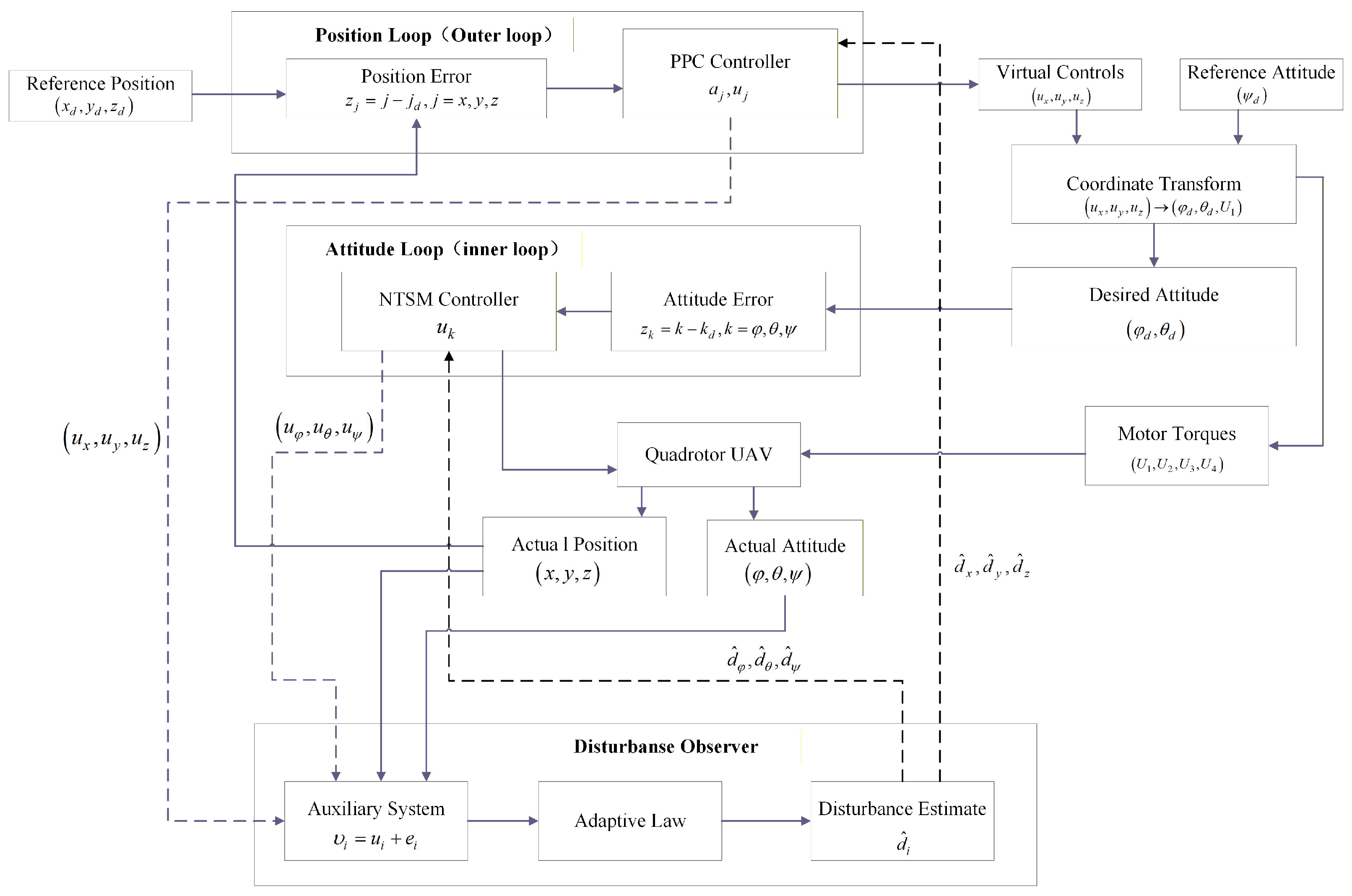
Based on the estimate of disturbance from the aforementioned disturbance observer, this section develops a QUAVs’ controller ensuring robust and accurate tracking with prescribed-time performance satisfaction. The hierarchical control structure is illustrated in Figure 1, which shows the outer position loop generating virtual controls $(u_x,u_y,u_z)$ via the PPC-based controller, the coordinate transformation converting these to desired attitude angles $({\phi }_d,{\theta }_d)$ and thrust $U_1$, the inner attitude loop using the NTSM controller to generate motor torques $(U_2,U_3,U_4)$, and the disturbance observer providing estimates ${\widehat{d}}_i$ to both controllers. (The solid line represents the real signal, and the dashed line represents the virtual signal).

4.1. Design of Prescribed-Time and Prescribed-Performance Controller for Position Loop

First, a prescribed-time control law for position control is designed for robust tracking. To accomplish the position system control objective, the position tracking error of the QUAVs is defined as follows:

$$z_x=x-x_d,z_y=y-y_d,z_z=z-z_d$$

(20)

where ${\left[z_x,z_y,z_z\right]}^T$ represents the position tracking error vector, ${\left[x_d,y_d,z_d\right]}^T$ includes the desired reference values for the three position components, and the actual output values for the three position components are ${\left[x,y,z\right]}^T$. The prescribed performance function can be designed as follows [28]:

$$p\left(t\right)=\left\{\begin{array}{c}\left(p_0-{\displaystyle \frac{t}{T_2}}\right)exp\left(1-{\displaystyle \frac{t}{T_2-t}}\right)+p_{\infty },0\le t<T_2\hfill \\ p_{\infty },t\ge T_2\hfill \end{array}\right.$$

(21)

where $p_0>1$ and $p_{\infty }$ are design parameters, and $T_2$ is a prescribed time parameter.

To render the prescribed performance control independent of initial conditions, the following function is introduced [29]:

$$\xi =\left\{\begin{array}{c}{\xi }_0+(1-{\xi }_0){\displaystyle \frac{1-cos\left(\frac{\pi t}{T_2}\right)}{2}},t<T_2\hfill \\ 1,t\ge T_2\hfill \end{array}\right.$$

(22)

Remark 3.

The smooth cosine transition function $\xi \left(t\right)$ with $\xi \left(0\right)={\xi }_0\approx 0$ (e.g., ${\xi }_0=0.001$) ensures: (1) Initial-condition decoupling: The transformed error $s_{j1}\left(0\right)={\xi }_0{z}_j\left(0\right)$ becomes arbitrarily small regardless of the magnitude of $z_j\left(0\right)$, guaranteeing $|s_{j1}\left(0\right)|<p\left(0\right)$ for any initial tracking error. (2) Continuity of control: The function satisfies $\xi \left(t\right)\in C^{\infty }$ for all $t\ge 0$, with $\dot{\xi }\left(t\right)={\displaystyle \frac{\pi (1-{\xi }_0)}{2T_2}}sin\left({\displaystyle \frac{\pi t}{T_2}}\right)$ continuous at $t=T_2$ (where $\dot{\xi }\left(T_2^{-}\right)=0=\dot{\xi }\left(T_2^{+}\right)$), eliminating discontinuities in control terms containing $\dot{\xi }$. For $t<T_2$, while $s_{j1}=\xi z_j$ grows with $\xi \left(t\right)$, the simultaneous decay of the performance bound $p\left(t\right)$ ensures that the constraint $|s_{j1}|<p\left(t\right)$ is maintained, which in turn bounds the physical error as $|z_j|<p\left(t\right)/\xi \left(t\right)$.

Then if we define

$$\left\{\begin{array}{c}{s}_{x1}=\xi z_x,s_{x2}=\dot{x}-{\alpha }_x\hfill \\ s_{y1}=\xi z_y,s_{y2}=\dot{y}-{\alpha }_y\hfill \\ s_{z1}=\xi z_z,s_{z2}=\dot{z}-{\alpha }_z\hfill \end{array}\right.,$$

(23)

it follows that their derivatives satisfy the following:

$$\left\{\begin{array}{c}{\dot{s}}_{x1}=\dot{\xi }{z}_x+\xi \left(\dot{x}-{\dot{x}}_d\right),{\dot{s}}_{x2}=u_x+d_x-{\dot{\alpha }}_x\hfill \\ {\dot{s}}_{y1}=\dot{\xi }{z}_y+\xi \left(\dot{y}-{\dot{y}}_d\right),{\dot{s}}_{y2}=u_y+d_y-{\dot{\alpha }}_y\hfill \\ {\dot{s}}_{z1}=\dot{\xi }{z}_z+\xi \left(\dot{z}-{\dot{z}}_d\right),{\dot{s}}_{z2}=u_z+d_z-{\dot{\alpha }}_z\hfill \end{array}\right..$$

(24)

Note that if the control law is designed such that

$$-p\left(t\right)<s_{j1}<p\left(t\right),j=x,y,z$$

(25)

it follows from $\xi \left(0\right)={\xi }_0\approx 0$ that $s_{j1}\left(0\right)={\xi }_0{z}_j\left(0\right)\approx 0$, which implies that $-p\left(0\right)<s_{j1}\left(0\right)<p\left(0\right)$ can be satisfied regardless of the value of $z_j\left(0\right)$, and after $T_2,s_j=\xi z_j$ always holds true.

To achieve the desired performance constraints, consider candidate Lyapunov functions with barriers designed as follows [29]:

$$V_{j1}={\displaystyle \frac{1}{2}}ln{\displaystyle \frac{p^2}{p^2-s_{j1}^2}},\left(j=x,y,z\right).$$

Lemma 3

(Boundedness of barrier Lyapunov function components). For the barrier Lyapunov function $V_{j1}={\displaystyle \frac{1}{2}}ln{\displaystyle \frac{p^2}{p^2-s_{j1}^2}}$ with $|s_{j1}|<p$, the following properties hold:

(i) The normalized error satisfies the following:

$${\displaystyle \frac{s_{j1}^2}{p^2-s_{j1}^2}}\ge 2V_{j1}$$

(ii) When $|s_{j1}|<p$, there exist positive constants ${\underline{\mathsf{\ell }}}_j$ and ${\overline{\mathsf{\ell }}}_j$ such that

$${\underline{\mathsf{\ell }}}_j\le \left|{\displaystyle \frac{s_{j1}}{p^2-s_{j1}^2}}\right|\le {\overline{\mathsf{\ell }}}_j.$$

(iii) For the performance function $p\left(t\right)$ defined in (21), there exists a constant ${\overline{M}}_p>0$ such that

$$\left|{\displaystyle \frac{\dot{p}\left(t\right)}{p\left(t\right)}}\right|\le {\overline{M}}_p,\forall t\ge 0.$$

Proof. 

(i) From the definition, $e^{2V_{j1}}={\displaystyle \frac{p^2}{p^2-s_{j1}^2}}$, which yields the following:

$$p^2-s_{j1}^2=p^2{e}^{-2V_{j1}}$$

Therefore,

$${\displaystyle \frac{s_{j1}^2}{p^2-s_{j1}^2}}={\displaystyle \frac{p^2-(p^2-s_{j1}^2)}{p^2-s_{j1}^2}}=e^{2V_{j1}}-1\ge 2V_{j1}$$

where the last inequality follows from $e^x\ge 1+x$ for all $x\in \mathbb{R}$.

(ii) Since $|s_{j1}|<p$ is maintained by the barrier, and $p\left(t\right)\ge p_{\infty }>0$, the function ${\mathsf{\ell }}_j\left(t\right)={\displaystyle \frac{s_{j1}}{p^2-s_{j1}^2}}$ is bounded.

(iii) Computing $\dot{p}\left(t\right)$ from (20) for $t<T_2$:

$$\dot{p}\left(t\right)=-{\displaystyle \frac{1}{T_2}}exp\left(1-{\displaystyle \frac{t}{T_2-t}}\right)+(p_0-{\displaystyle \frac{t}{T_2}})exp\left(1-{\displaystyle \frac{t}{T_2-t}}\right)·{\displaystyle \frac{T_2}{{(T_2-t)}^2}}.$$

Since $p\left(t\right)\ge p_{\infty }$, the ratio $|\dot{p}/p|$ remains bounded for all $t\ge 0$. □

It follows that

$$\begin{array}{cc}{\dot{V}}_{j1}\hfill & ={\displaystyle \frac{s_{j1}}{p^2-s_{j1}^2}}\left({\dot{s}}_{j1}-\dot{p}{s}_{j1}/p\right)\hfill \\ \hfill & ={\mathsf{\ell }}_j\left(\dot{\xi }{z}_j+\xi \left(s_{j2}+{\alpha }_j-{\dot{j}}_d\right)-\dot{p}{s}_{j1}/p\right)\hfill \\ \hfill & ={\mathsf{\ell }}_j\xi \left(s_{j2}+{\alpha }_j-{\dot{j}}_d\right)+{\mathsf{\ell }}_j\left(\dot{\xi }{z}_j-\dot{p}{s}_{j1}/p\right),\hfill \end{array}$$

(26)

where ${\mathsf{\ell }}_j={\displaystyle \frac{s_{j1}}{p^2-s_{j1}^2}}$.

According to Young’s inequality, for any ${\lambda }_j>0$, we have the following:

$$-{\mathsf{\ell }}_j\dot{p}{s}_{j1}/p\le {\displaystyle \frac{{\mathsf{\ell }}_j^2{s}_{j1}^2}{2{\lambda }_j}}{\displaystyle \frac{{\dot{p}}^2}{p^2}}+{\displaystyle \frac{{\lambda }_j}{2}}$$

By Lemma 3(ii) and (iii), there exists ${\rho }_{j1}>0$ such that

$${\displaystyle \frac{{\mathsf{\ell }}_j^2{s}_{j1}^2}{2{\lambda }_j}}{\displaystyle \frac{{\dot{p}}^2}{p^2}}\le {\rho }_{j1}$$

for all $t\ge 0$ and all $|s_{j1}|<p$.

By plugging it into (26), we can obtain the following:

$${\dot{V}}_{j1}\le {\mathsf{\ell }}_j\xi \left(s_{j2}+{\alpha }_j-{\dot{j}}_d+{\displaystyle \frac{{\mathsf{\ell }}_j\xi z_j^2}{2{\lambda }_j}}{\displaystyle \frac{{\dot{p}}^2}{p^2}}\right)+{\rho }_{j1}+{\displaystyle \frac{{\lambda }_j}{2}}+{\mathsf{\ell }}_j\dot{\xi }{z}_j$$

(27)

By designing the position loop virtual control rate as

$${\alpha }_j=-{\mu }_{j1}{s}_{j1}+{\dot{j}}_d-{\displaystyle \frac{{\mathsf{\ell }}_j\xi z_j^2}{2{\lambda }_j}}{\displaystyle \frac{{\dot{p}}^2}{p^2}},$$

(28)

where ${\mu }_{j1}$ is the regularization parameter, it follows from (27) that

$${\dot{V}}_{j1}\le -{\mu }_{j1}\xi {\displaystyle \frac{s_{j1}^2}{p^2-s_{j1}^2}}+{\rho }_{j1}+{\displaystyle \frac{{\lambda }_j}{2}}+{\mathsf{\ell }}_j\xi s_{j2}+{\mathsf{\ell }}_j\dot{\xi }{z}_j.$$

To further design the stabilizing control law, let us consider candidate Lyapunov functions given as $V_{j2}=V_{j1}+{\displaystyle \frac{1}{2}}{s}_{j2}^2$, whose derivatives satisfy the following:

$${\dot{V}}_{j2}={\dot{V}}_{j1}+s_{j2}{\dot{s}}_{j2}={\dot{V}}_{j1}+s_{j2}\left(u_j+d_j-{\dot{\alpha }}_j\right)$$

(29)

To eliminate the problematic singular term, we employ the following continuous approximation. Note that

$${\mathsf{\ell }}_j\dot{\xi }{z}_j{s}_{j2}={\mathsf{\ell }}_j\dot{\xi }{z}_j{s}_{j2}·{\displaystyle \frac{s_{j2}^2+{\delta }_j^2}{s_{j2}^2+{\delta }_j^2}},$$

where ${\delta }_j>0$ is a small design parameter. This allows us to write the following:

$${\mathsf{\ell }}_j\dot{\xi }{z}_j={\mathsf{\ell }}_j\dot{\xi }{z}_j·{\displaystyle \frac{s_{j2}}{s_{j2}^2+{\delta }_j^2}}·s_{j2}$$

The control law is thus designed as follows:

$$u_j=-{\mu }_{j2}{s}_{j2}-{\widehat{d}}_j+{\dot{\alpha }}_j-{\mathsf{\ell }}_j\xi -{\mathsf{\ell }}_j\dot{\xi }{z}_j{\displaystyle \frac{s_{j2}}{s_{j2}^2+{\delta }_j^2}},$$

(30)

where ${\mu }_{j2}\left(j=x,y,z\right)$ is the regularization parameter and ${\delta }_j>0$ is a small positive constant that prevents singularity when $s_{j2}\to 0$.

Remark 4.

The continuous approximation ${\displaystyle \frac{s_{j2}}{s_{j2}^2+{\delta }_j^2}}$ ensures the following: (1) The control law remains bounded for all $s_{j2}$, including $s_{j2}=0$; (2) When $|s_{j2}|\gg {\delta }_j$, the approximation ${\displaystyle \frac{s_{j2}}{s_{j2}^2+{\delta }_j^2}}\approx s_{j2}^{-1}$ closely matches the original design intent; (3) The approximation error ${\mathsf{\ell }}_j\dot{\xi }{z}_j{\displaystyle \frac{{\delta }_j^2}{s_{j2}^2+{\delta }_j^2}}$ is uniformly bounded and can be made arbitrarily small by choosing ${\delta }_j$ sufficiently small, while maintaining control continuity.

Theorem 2.

Consider the quadrotor UAV position subsystem described by (6) with the prescribed-time disturbance observer (8)–(12) and the position control law (19)–(30). Suppose the following conditions hold:

1. The desired trajectory is bounded and twice differentiable;

2. The observer parameters satisfy $\alpha >0,\beta >0,0<\gamma <1$;

3. The controller parameter $p_0>1$;

4. The prescribed time parameters satisfy $T_1>0,T_2>0$; and the approximation parameter ${\delta }_j>0$.

Then, the position tracking error converges to a small neighborhood of the prescribed performance bounds within the prescribed time, specifically: (i) the performance constraint $|s_{j1}\left(t\right)|<p\left(t\right)$ is satisfied for all $t\ge 0$, ensuring $|z_j\left(t\right)|<p\left(t\right)/\xi \left(t\right)$; and (ii) for $t\ge T_2$, the system exhibits exponential ultimate boundedness with $|z_j\left(t\right)|\le p_{\infty }+\mathcal{O}\left(\sqrt{{\mathsf{\Theta }}_j/{\mu }_j}\right)$, where the bound ${\mathsf{\Theta }}_j$ depends on disturbance observation error, control approximation error, and performance function derivative.

Remark 5.

The term “arbitrary initial conditions” in this paper refers to a theoretical framework where the control method can handle a wide range of initial states. In practical UAV applications, the initial conditions are naturally constrained by physical limitations. Therefore, “arbitrary initial conditions” should be interpreted as “high-redundancy initial conditions”.

Proof. 

Substituting the control law (30) into (29):

$$\begin{array}{cc}{\dot{V}}_{j2}\hfill & \le -{\mu }_{j1}\xi {\displaystyle \frac{s_{j1}^2}{p^2-s_{j1}^2}}-{\mu }_{j2}{s}_{j2}^2+{\rho }_{j1}+{\displaystyle \frac{{\lambda }_j}{2}}+{\mathsf{\ell }}_j\dot{\xi }{z}_j{\displaystyle \frac{{\delta }_j^2}{s_{j2}^2+{\delta }_j^2}}+s_{j2}{\tilde{d}}_j\hfill \end{array}$$

(31)

Using Young’s inequality on $s_{j2}{\tilde{d}}_j$:

$$s_{j2}{\tilde{d}}_j\le {\displaystyle \frac{s_{j2}^2}{2{ϵ}_j}}+{\displaystyle \frac{{ϵ}_j{\tilde{d}}_j^2}{2}}$$

and noting that ${\displaystyle \frac{{\delta }_j^2}{s_{j2}^2+{\delta }_j^2}}\le 1$ and by Lemma 3(ii) $|{\mathsf{\ell }}_j|\le {\overline{\mathsf{\ell }}}_j$, we have the following:

$${\mathsf{\ell }}_j\dot{\xi }{z}_j{\displaystyle \frac{{\delta }_j^2}{s_{j2}^2+{\delta }_j^2}}\le {\overline{\mathsf{\ell }}}_j|\dot{\xi }\left|\right|z_j|\le {\rho }_{j2}$$

for some constant ${\rho }_{j2}>0$ (since $\dot{\xi }$ and $z_j$ remain bounded in the closed-loop system).

Therefore,

$${\dot{V}}_{j2}\le -{\mu }_{j1}\xi {\displaystyle \frac{s_{j1}^2}{p^2-s_{j1}^2}}-\left({\mu }_{j2}-{\displaystyle \frac{1}{2{ϵ}_j}}\right)s_{j2}^2+{\mathsf{\Theta }}_j,$$

(32)

where ${\mathsf{\Theta }}_j={\rho }_{j1}+{\rho }_{j2}+{\displaystyle \frac{{\lambda }_j}{2}}+{\displaystyle \frac{{ϵ}_j{D}_{max}^2}{2}}$ (using the bound from Theorem 1 on $|{\tilde{d}}_j|\le \epsilon$ for sufficiently large t).

By Lemma 3(i):

$$\begin{array}{cc}{\dot{V}}_{j2}\hfill & \le -2{\mu }_{j1}\xi V_{j1}-\left({\mu }_{j2}-{\displaystyle \frac{1}{2{ϵ}_j}}\right)s_{j2}^2+{\mathsf{\Theta }}_j\hfill \\ \hfill & \le -{\mu }_j{V}_{j2}+{\mathsf{\Theta }}_j\hfill \end{array}$$

(33)

where ${\mu }_j=min\left\{2{\mu }_{j1}{\xi }_{min},2\left({\mu }_{j2}-{\displaystyle \frac{1}{2{ϵ}_j}}\right)\right\}>0$ (provided ${\mu }_{j2}>{\displaystyle \frac{1}{2{ϵ}_j}}$, which can be satisfied by design), and ${\xi }_{min}={\xi }_0>0$ is the minimum value of $\xi \left(t\right)$. By integrating both sides of (33), we have the following:

$$V_{j2}\le \left(V_{j2}\left(0\right)-{\displaystyle \frac{{\mathsf{\Theta }}_j}{{\mu }_j}}\right)exp\left(-{\mu }_{j}t\right)+{\displaystyle \frac{{\mathsf{\Theta }}_j}{{\mu }_j}}$$

(34)

By substituting the aforementioned expression into Equation (33), it can be inferred that ${\dot{V}}_{j2}\le 0$. Since

$$\begin{array}{c}{V}_{j2}=V_{j1}+\left(1/2\right){s_{j2}}^2=\left(1/2\right)ln\left[p^2/\left(p^2-{s_{j1}}^2\right)\right]+1/2{s_{j2}}^2\hfill \\ \le A{e}^{\left(-{\mu }_{j}t\right)}+B,\hfill \end{array}$$

where $A=V_{j2}\left(0\right)-{\displaystyle \frac{{\mathsf{\Theta }}_j}{{\mu }_j}},B={\displaystyle \frac{{\mathsf{\Theta }}_j}{{\mu }_j}}$, then

$$\begin{array}{c}ln\left[p^2/\left(p^2-s_{j1}^2\right)\right]\le 2A{e}^{\left(-{\mu }_{j}t\right)}+2B\hfill \\ p^2/\left(p^2-s_{j1}^2\right)\le e^{2A{e}^{\left(-{\mu }_{j}t\right)}+2B}\hfill \\ C\left(t\right){s_{j1}}^2\le \left(C\left(t\right)-1\right)p^2\hfill \end{array}$$

in which $C\left(t\right)=e^{2A{e}^{\left(-{\mu }_{j}t\right)}+2B}$. Therefore, ${s_{j1}}^2\le p^2$. In this case, prescribed performance $-p\left(t\right)<s_{j1}<p\left(t\right)$ holds, and the system states converge to a small neighborhood of the origin. □

Remark 6.

(Clarification on Performance Satisfaction)

The proposed method achieves two distinct aspects:

(i) Prescribed-time performance constraint satisfaction: The barrier Lyapunov function guarantees $|s_{j1}\left(t\right)|<p\left(t\right)$ for all $t\ge 0$, where $p\left(t\right)$ decreases from $p_0$ to $p_{\infty }$ within time $T_2$. This ensures the physical tracking error satisfies $|z_j\left(t\right)|<p\left(t\right)/\xi \left(t\right)$, achieving bounded tracking within the prescribed time $T_2$ regardless of initial conditions.

(ii) Exponential ultimate boundedness: The inequality ${\dot{V}}_{j2}\le -{\mu }_j{V}_{j2}+{\mathsf{\Theta }}_j$ (Equation (33)) yields exponential convergence to an ultimate bound ${lim}_{t\to \infty }{V}_{j2}\left(t\right)\le {\mathsf{\Theta }}_j/{\mu }_j$, rather than exact convergence to zero. The bound ${\mathsf{\Theta }}_j$ arises from three sources: (a) disturbance observation error $|{\tilde{d}}_j|\le \epsilon$ (Theorem 1), (b) continuous approximation error ${\rho }_{j2}$ from the term ${\delta }_j^2/(s_{j2}^2+{\delta }_j^2)$ (Equation (30)), and (c) performance function derivative bound ${\rho }_{j1}$ (Lemma 3).

(iii) Engineering rationale for $p_{\infty }>0$: Setting $p_{\infty }=0$ would theoretically require infinite control gains at $t=T_2$, which is impractical given actuator saturation. The design choice $p_{\infty }>0$ provides the following: (a) bounded control effort, (b) robustness to persistent disturbances and modeling uncertainties, and (c) adjustable steady-state accuracy through parameter tuning ($a_3$, ${\delta }_j$, ${ϵ}_j$, ${\mu }_j$). The ultimate bound can be made arbitrarily small by appropriate parameter selection.

4.2. Design of Sliding Mode Controller for Prescribed-Time Attitude Loop

Considering the characteristics of the QUAV’s attitude dynamics, applying a prescribed-time terminal sliding mode controller that is different from the controller used for the position loop can be more effective for rapid and robust stabilization of the attitude loop.

To design and analyze the controller, the errors in attitude tracking of a quadrotor UAV are defined as follows:

$$z_{\phi }=\phi -{\phi }_d,z_{\theta }=\theta -{\theta }_d,z_{\Psi }=\Psi -{\Psi }_d,$$

(35)

where ${\left[{\phi }_d,{\theta }_d,{\Psi }_d\right]}^T$ is the reference attitude input vector, and ${\left[\phi ,\theta ,\Psi \right]}^T$ is the actual output attitude angle information. The derivatives of errors in (35) can be obtained by the following:

$${\dot{z}}_{\phi }=\dot{\phi }-{\dot{\phi }}_d,{\dot{z}}_{\theta }=\dot{\theta }-{\dot{\theta }}_d,{\dot{z}}_{\Psi }=\dot{\Psi }-{\dot{\Psi }}_d$$

(36)

where ${\left[{\dot{z}}_{\phi },{\dot{z}}_{\theta },{\dot{z}}_{\Psi }\right]}^T,{\left[{\dot{\phi }}_d,{\dot{\theta }}_d,{\dot{\Psi }}_d\right]}^T$, and ${\left[\dot{\phi },\dot{\theta },\dot{\Psi }\right]}^T$ represent the derivatives of ${\left[z_{\phi },z_{\theta },z_{\Psi }\right]}^T,$${\left[{\phi }_d,{\theta }_d,{\Psi }_d\right]}^T$, and ${\left[\phi ,\theta ,\Psi \right]}^T$, respectively.

The prescribed-time non-singular terminal sliding mode surface for the attitude control system is designed as [26]:

$$s_k={\dot{z}}_k+b_{1}sign\left(z_k\right){\left|z_k\right|}^{1-{\gamma }_2}+b_{2}sign\left(z_k\right){\left|z_k\right|}^{1+{\gamma }_2}\left(k=\phi ,\theta ,\Psi \right)$$

(37)

where the parameters satisfy the following:

$$\begin{array}{c}{b}_1={\displaystyle \frac{\pi {\eta }_2^{1/2}}{{\gamma }_2{T}_3{\beta }_2^{1/2}}}{\left({\displaystyle \frac{1}{2}}\right)}^{1-{\displaystyle \frac{{\gamma }_2}{2}}},b_2={\displaystyle \frac{\pi {\beta }_2^{1/2}}{{\gamma }_2{T}_3{\eta }_2^{1/2}}}{\left({\displaystyle \frac{1}{2}}\right)}^{1+{\displaystyle \frac{{\gamma }_2}{2}}},\hfill \\ {\gamma }_2\in \left(0,1\right),{\eta }_2>0,{\beta }_2>0.\hfill \end{array}$$

Remark 7.

The prescribed-time property is directly embedded in the sliding surface design (Equation (37)) through the power-law coefficients $b_1$ and $b_2$, which are explicitly functions of the prescribed time $T_3$. Specifically, when the system reaches the sliding surface $s_k=0$, the dynamics become the following:

$${\dot{z}}_k+b_1\mathit{sign}\left(z_k\right)|z_k{|}^{1-{\gamma }_2}+b_2\mathit{sign}\left(z_k\right){\left|z_k\right|}^{1+{\gamma }_2}=0$$

The above formulation for the sliding mode surface structure, combined with the specific parameter selection of $b_1$ and $b_2$, guarantees convergence from any point on the sliding surface to a neighborhood of the origin within time $T_3$, as proven in Theorem 3.

It can be derived that

$${\dot{s}}_k=u_k+d_k-{\ddot{k}}_d+{\varsigma }_k{\dot{z}}_k,$$

(38)

where ${\varsigma }_k=\left(1-{\gamma }_2\right)b_1{\left|z_k\right|}^{-{\gamma }_2}+\left(1+{\gamma }_2\right)b_2{\left|z_k\right|}^{{\gamma }_2}$.

To design the control law and guarantee stability, consider candidate Lyapunov functions defined as $V_k={\displaystyle \frac{1}{2}}{s}_k^2,k=\phi ,\theta ,\Psi$. The derivatives of these functions satisfy the following:

$${\dot{V}}_k=s_k\left(u_k+d_k-{\ddot{k}}_d+{\varsigma }_k{\dot{z}}_k\right)$$

(39)

Now, we are motivated to design the observer-based sliding mode controller as follows:

$$u_k=I_j\left(\begin{array}{c}-c_{1}sign\left(s_k\right){\left|s_k\right|}^{1-{\gamma }_3}-\hfill \\ c_{2}sign\left(s_k\right){\left|s_k\right|}^{1+{\gamma }_3}\hfill \\ -c_3{s}_k-{\widehat{d}}_k+{\ddot{k}}_d-{\varsigma }_k{\dot{z}}_k\hfill \end{array}\right)$$

(40)

where the parameters satisfy the following:

$$\begin{array}{c}{c}_1={\displaystyle \frac{\pi {\eta }_3^{1/2}}{{\gamma }_3{T}_3{\beta }_3^{1/2}}}{\left({\displaystyle \frac{1}{2}}\right)}^{1-{\displaystyle \frac{{\gamma }_3}{2}}},c_2={\displaystyle \frac{\pi {\beta }_3^{1/2}}{{\gamma }_3{T}_3{\eta }_3^{1/2}}}{\left({\displaystyle \frac{1}{2}}\right)}^{1+{\displaystyle \frac{{\gamma }_3}{2}}},\hfill \\ c_3>0,{\gamma }_3\in \left(0,1\right),{\eta }_3>0,{\beta }_3>0.\hfill \end{array}$$

The stability property of the proposed attitude control law is demonstrated in the following theorem.

Theorem 3.

Consider the quadrotor UAV attitude subsystem (35) and (36), with the prescribed-time non-singular terminal sliding-mode surface (37) and the attitude control law (40). Suppose the following conditions hold:

1. The desired attitude trajectories are bounded and differentiable;

2. The observer parameters satisfy $\alpha >0,\beta >0,0<\gamma <1$;

3. The sliding mode surface parameters satisfy ${\gamma }_2\in \left(0,1\right),{\eta }_2>0,{\beta }_2>0$, and the controller parameters satisfy $c_3>0,{\gamma }_3\in \left(0,1\right),{\eta }_3>0,{\beta }_3>0.$

4. The prescribed time parameters satisfy $T_1>0,T_3>0$.

Then the attitude tracking error vector converges to a small neighborhood of the origin within the prescribed time, specifically: the sliding variable $s_k\left(t\right)$ reaches a neighborhood of zero within time $T_3$, and consequently $z_k\left(t\right)$ is ultimately bounded with $\mathcal{O}\left(\sqrt{{ϵ}_k{\epsilon }^2/c_3}\right)$ for $t\ge T_3$, where ε is the disturbance observation bound from Theorem 1.

Proof. 

Substituting (40) into (39) and using ${\tilde{d}}_k=d_k-{\widehat{d}}_k$:

$${\dot{V}}_k=s_k(-c_{1}sign\left(s_k\right)|s_k{|}^{1-{\gamma }_3}-c_{2}sign\left(s_k\right)|s_k{|}^{1+{\gamma }_3}-c_3{s}_k+{\tilde{d}}_k)$$

(41)

Using Young’s inequality on $s_k{\tilde{d}}_k$:

$$s_k{\tilde{d}}_k\le {\displaystyle \frac{s_k^2}{2{ϵ}_k}}+{\displaystyle \frac{{ϵ}_k{\tilde{d}}_k^2}{2}}$$

Therefore,

$$\begin{array}{cc}{\dot{V}}_k\hfill & \le -c_1|s_k{|}^{2-{\gamma }_3}-c_2{\left|s_k\right|}^{2+{\gamma }_3}-\left(c_3-{\displaystyle \frac{1}{2{ϵ}_k}}\right)s_k^2+{\displaystyle \frac{{ϵ}_k{\epsilon }^2}{2}}\hfill \\ \hfill & \le -c_1{\left(2V_k\right)}^{{\displaystyle \frac{2-{\gamma }_3}{2}}}-c_2{\left(2V_k\right)}^{{\displaystyle \frac{2+{\gamma }_3}{2}}}-\left(c_3-{\displaystyle \frac{1}{2{ϵ}_k}}\right)2V_k+{\displaystyle \frac{{ϵ}_k{\epsilon }^2}{2}},\hfill \end{array}$$

(42)

where we used the observer bound $|{\tilde{d}}_k|\le \epsilon$ from Theorem 1 for sufficiently large t.

For the appropriate choice of ${ϵ}_k$ such that $c_3>{\displaystyle \frac{1}{2{ϵ}_k}}$, the dominant terms yield the following:

$${\dot{V}}_k\le -{\displaystyle \frac{\pi }{{\gamma }_3{T}_3\sqrt{{\eta }_3{\beta }_3}}}\left({\eta }_3{V}_k^{1-{\displaystyle \frac{{\gamma }_3}{2}}}+{\beta }_3{V}_k^{1+{\displaystyle \frac{{\gamma }_3}{2}}}\right)+{\displaystyle \frac{{ϵ}_k{\epsilon }^2}{2}}.$$

(43)

According to Lemma 1, the system state vector reaches a small neighborhood of the sliding mode surface within a prescribed time $T_3$. Hence, the control system can converge to a small neighborhood of the origin within prescribed time $T=max\left\{T_1,T_2,T_3\right\}$. □

Remark 8.

The ultimate bounds in both position and attitude loops can be made arbitrarily small by: (1) Increasing the observer gain $a_3$ to reduce ε; (2) Reducing the approximation parameter ${\delta }_j$ in the position controller; (3) Adjusting ${ϵ}_j$ and ${ϵ}_k$ to balance convergence rate and steady-state accuracy. In practice, these parameters are tuned to achieve desired tracking performance while maintaining control smoothness.

5. Numerical Experiments

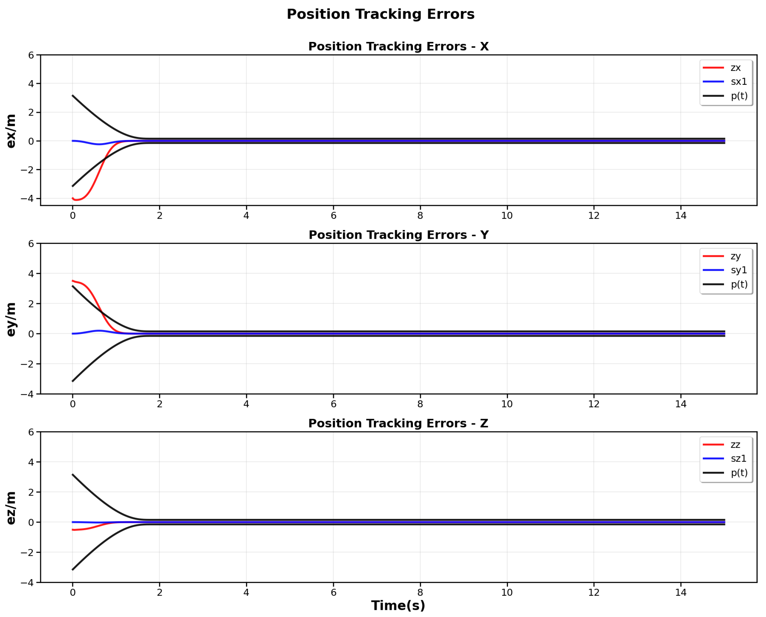
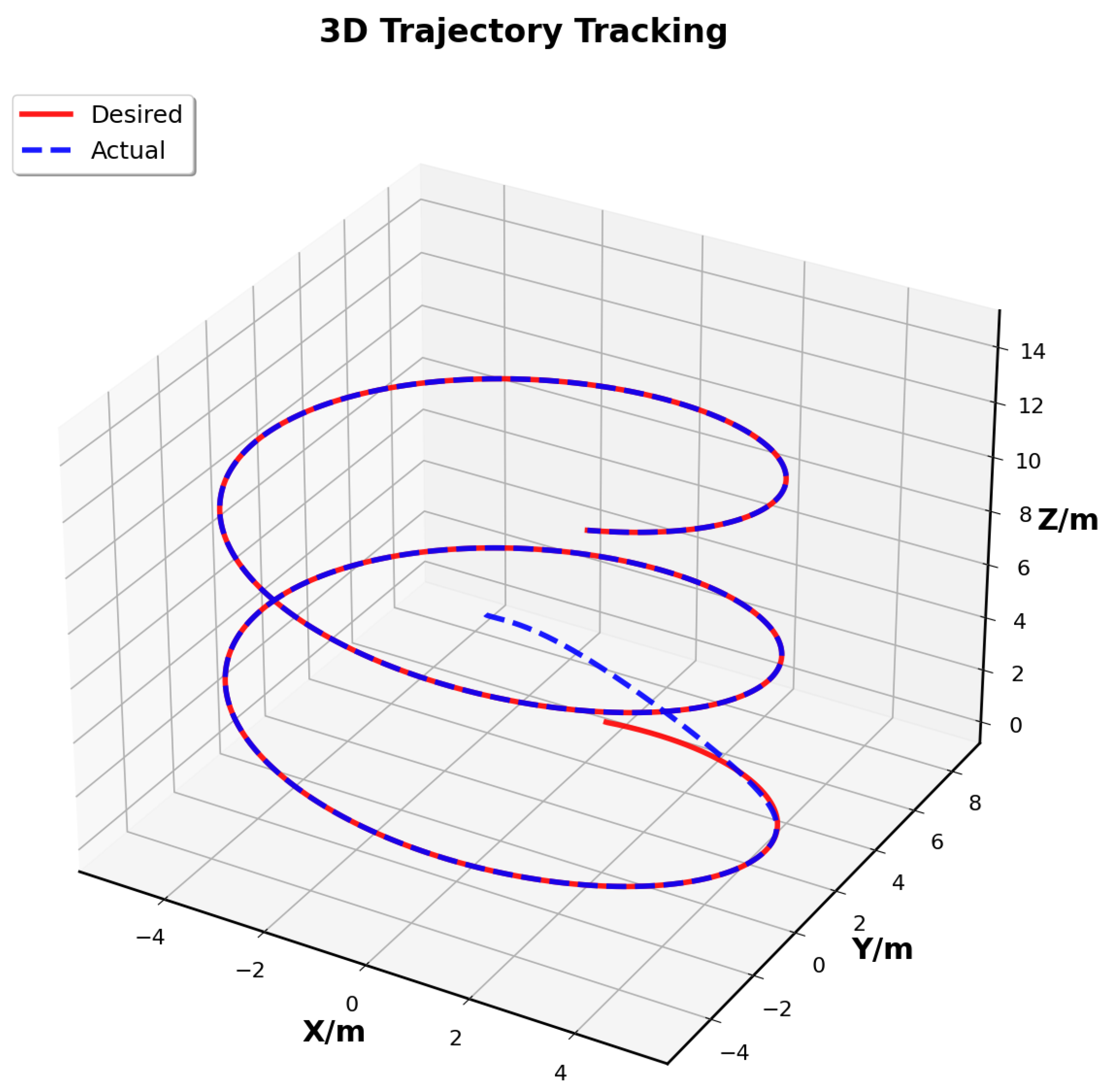
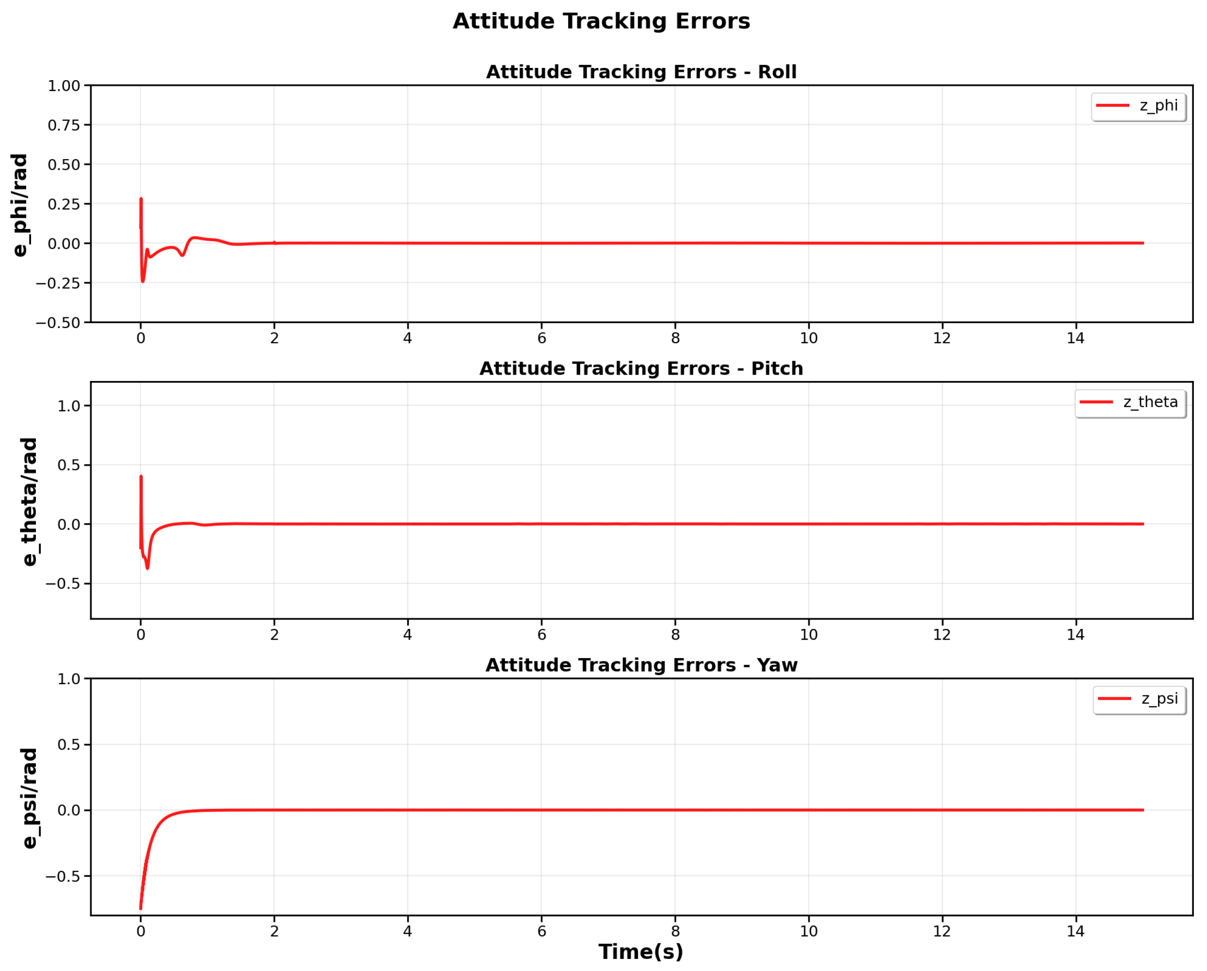
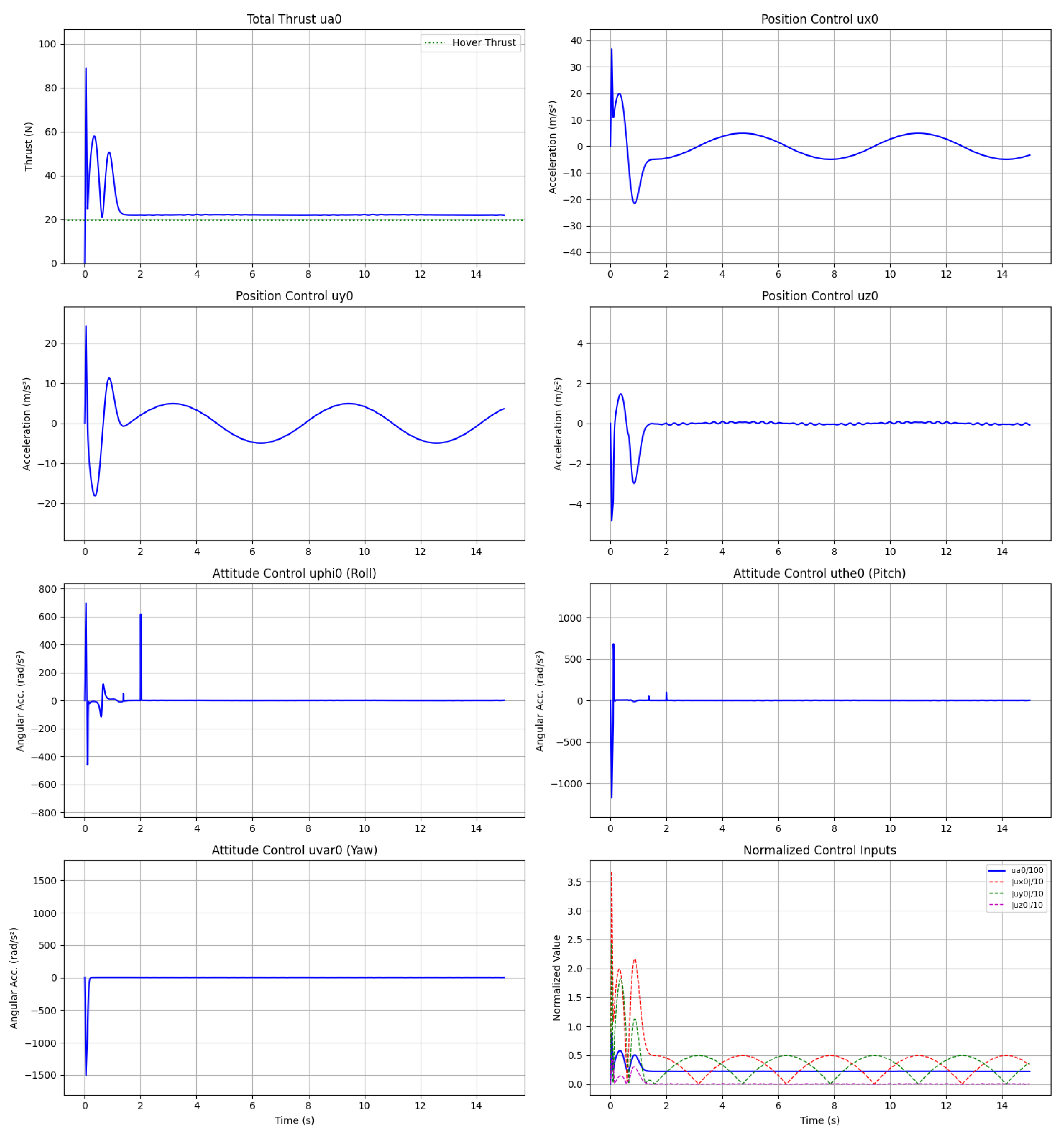
To verify the effectiveness of the proposed control method, simulations are carried out with designed parameters given in

Table 1. Simulation parameters.

Parameters	Value
Simulation	$m=2,I_x=I_y=1.24,I_z=2.5$,
Parameters	$K_x=K_y=K_z=K_{\phi }=K_{\theta }=K_{\psi }=0.01$
Disturbance	$f_i=0.1sin\left(0.01t\right)sin\left(0.1t\right)+0.1sin\left(i\right)$ Type: Matched, time-varying, bounded Magnitude: $|f_i\left(t\right)|\le 0.2$ for all i
Reference signal	$x_d=5sin\left(t\right),y_d=5cos\left(t\right),z_d=t,{\phi }_d=\pi /3$
Initial state	$x=-4,y=8.5,z=-0.5$, $\phi =0.1,\theta =-0.2,\psi =0.3$
Prescribed time	$T_1=1,T_2=3,T_3=1$
PPC function parameters	$p_0=1.1,p_{\infty }=0.15,{\xi }_0=0.001$
Observer parameters	${\gamma }_1=0.5,{\eta }_1=0.1,{\beta }_1=0.5,a3=5$
Controller parameters	${\mu }_{j1}=30,{\mu }_{j2}=35,{\lambda }_j=50,{\delta }_j=0.01$, ${\gamma }_2=0.3,{\eta }_2=0.1,{\beta }_2=2$, ${\gamma }_3=0.3,{\eta }_3=6,{\beta }_3=5,b_3=20$

. Results show that the method in this paper can solve the trajectory tracking problem under composite disturbances within a prescribed time. As shown in Figure 2, the QUAV used in the simulation is able to track the desired trajectory by utilizing the control method proposed in this paper. Figure 3 shows that the position error converges to a small neighborhood of the origin within the user’s prescribed time, and Figure 4 shows that the attitude error converges to a small neighborhood of the origin within the prescribed time as well. It can be seen that the proposed method exhibits superior convergence accuracy when handling large initial deviations and strong composite disturbances, and that the convergence time constraints and robust stability are strictly satisfied. Figure 5 depicts the control inputs signals of position and altitude. The applied disturbances are matched (directly added to control channels via Equation (1)), time-varying (containing periodic sinusoidal components), and bounded with magnitude $|f_i\left(t\right)|\le 0.2$ for all channels. The disturbance model $f_i=0.1sin\left(0.01t\right)sin\left(0.1t\right)+0.1sin\left(i\right)$ captures both slow-varying environmental effects (wind gusts with 0.01 Hz modulation) and high-frequency oscillations (sensor noise at 0.1 Hz), representing realistic operational conditions for small quadrotors.

5.1. Results Analysis

The actual position trajectories $(x,y,z)$ closely follow their references $(x_d,y_d,z_d)$ after the transient period, with steady-state errors remaining below the prescribed bounds. Similarly, the attitude angles $(\phi ,\theta ,\psi )$ track their desired values with errors converging to small neighborhoods. These tracking accuracies are adequate for typical autonomous flight missions such as waypoint navigation and trajectory following.

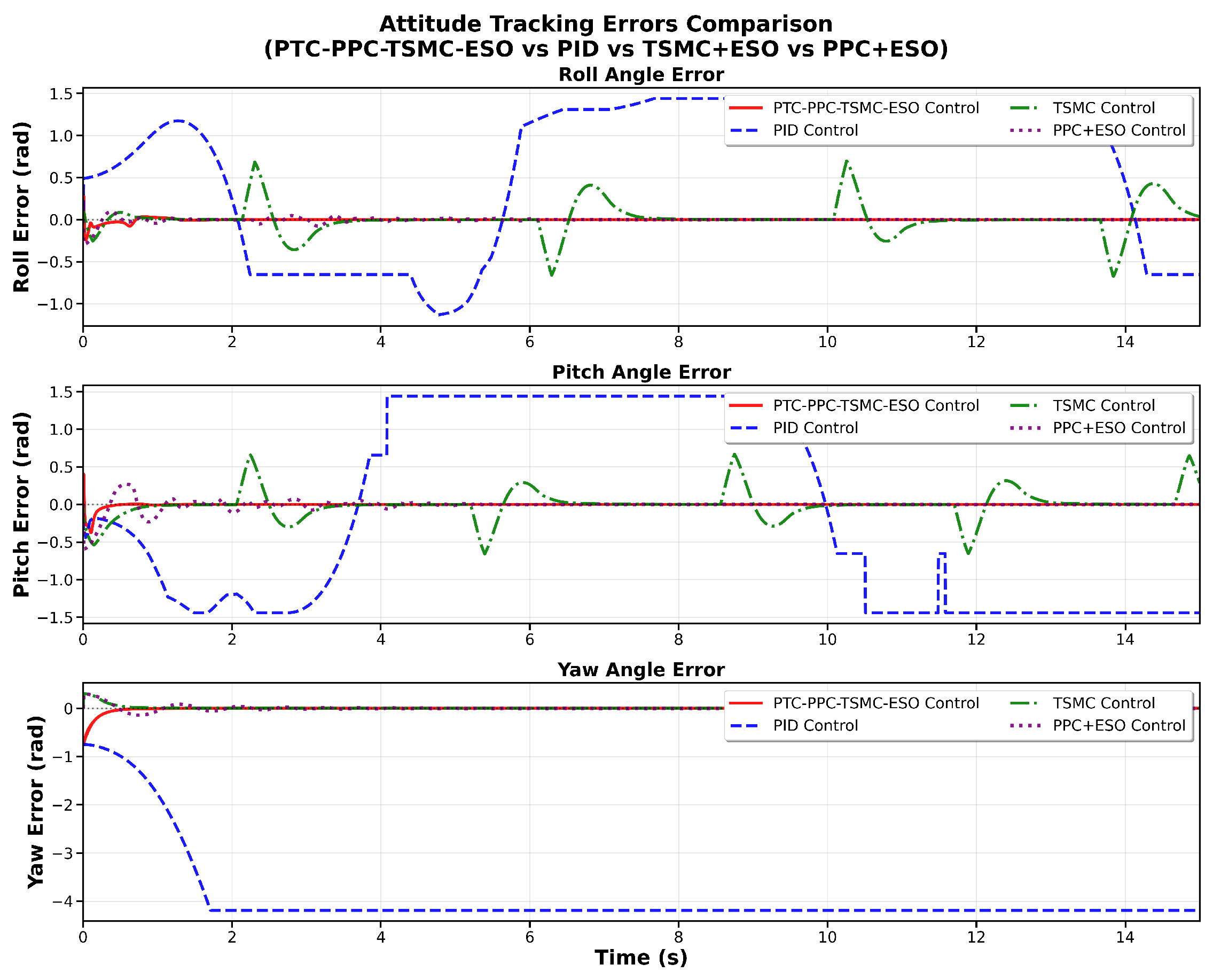
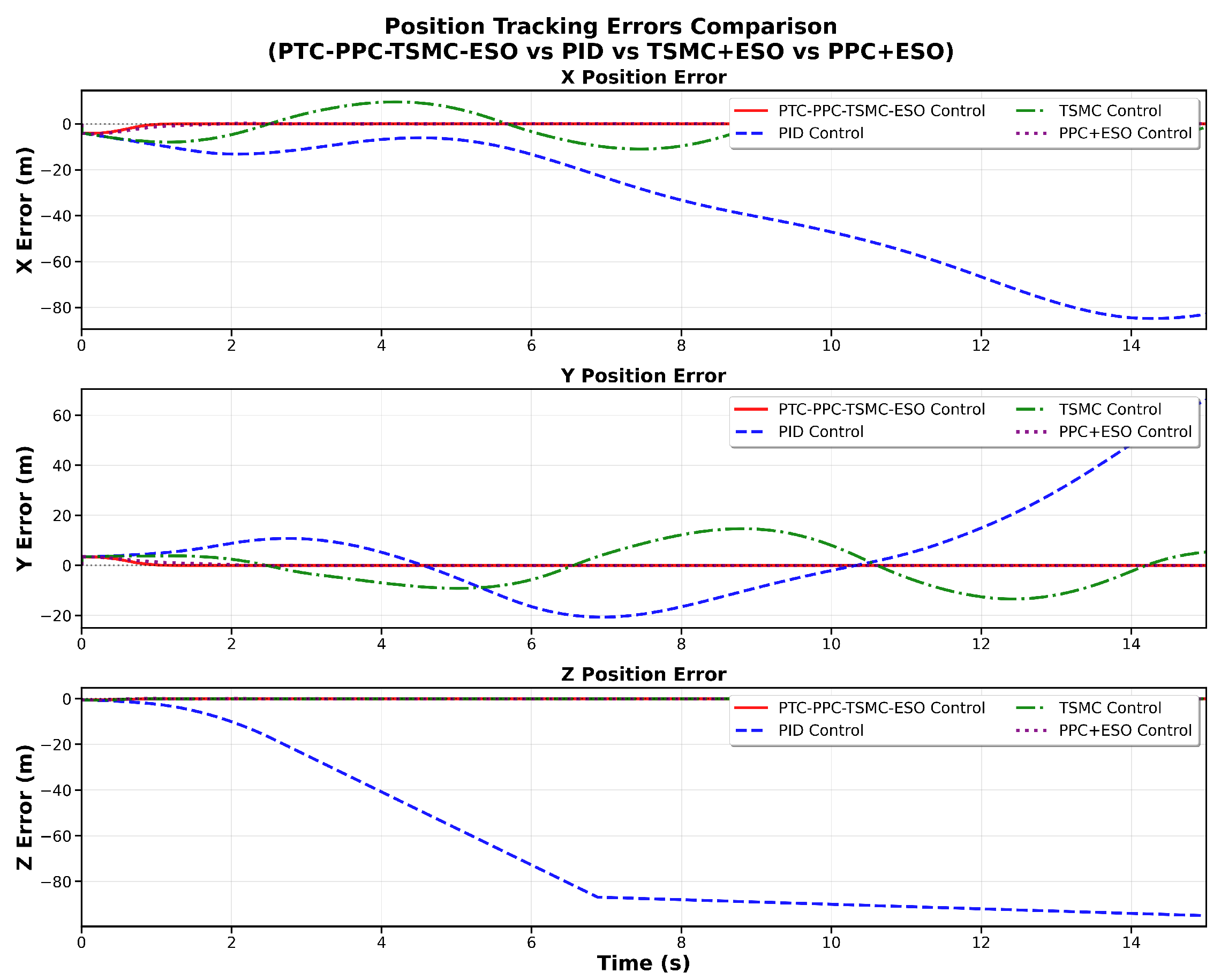
This paper conducts a comparative analysis of four different methods (results are shown in Figure 6 and Figure 7): PID control, terminal sliding mode control with extended state observer (TSMC-ESO), combination of prescribed performance control with extended state observer (PPC-ESO), and the method proposed in this paper (PTC-PPC-TSMC-ESO). It can be observed that the PID controller is insufficient to control the system in the presence of time-varying disturbances. The TSMC-ESO method exhibits suboptimal performance in the position loop control, but it can converge quickly in the attitude loop; however, the use of a sign function in the switching rate causes oscillations about the origin. The PPC-ESO method performs well in position loop control, but in the attitude loop, the convergence rate is unsatisfactory, and the states exhibit large fluctuations. Based on the comparison, the proposed method, which combines PPC, PTC, TSMC, and ESO, can significantly mitigate the shortcomings of the aforementioned methods, leading to substantial improvements in QUAV control under disturbances.

5.2. Limitations and Future Directions

Despite the theoretical contributions and promising simulation results, several limitations of the proposed method should be acknowledged:

1. Need for systematic parameter tuning guidelines: The method involves the adjustment of over a dozen parameters across the observer and controllers. Although effective parameter sets have been demonstrated in simulation, systematic and efficient tuning strategies for different quadrotor platforms and mission profiles require further study and clear guidelines to facilitate practical deployment.

2. Higher real-time computational demand: The real-time computation of the disturbance observer and the derivatives of the barrier Lyapunov function imposes greater processing requirements compared to conventional PID controllers. Deployment on embedded hardware with sufficient computing power is necessary to maintain control rates above 100 Hz.

3. Dependence on model parameters: The control design relies on accurate model parameters such as moments of inertia $I_x,I_y,I_z$ and drag coefficients $K_i$. While the disturbance observer enhances robustness to parametric uncertainties to some extent, control performance may still degrade when model errors are significant (e.g., exceeding $\pm 20\%$).

Future research directions:

• Experimental validation: Hardware-in-the-loop (HIL) testing and flight experiments on physical quadrotor platforms to validate control performance under real-world conditions, including sensor noise, actuator delays, and aerodynamic effects.
• Adaptive parameter tuning: Development of online learning algorithms (e.g., reinforcement learning or adaptive control) to automatically adjust controller gains based on flight conditions and disturbance characteristics.
• Extension to multi-UAV systems: Application of the proposed framework to cooperative control of heterogeneous multi-UAV formations with communication constraints, as motivated by recent work on resilient distributed control [9].
• Integration with perception systems: Combination of the proposed control with vision-based state estimation and obstacle avoidance for fully autonomous navigation in GPS-denied environments.

These directions aim to bridge the gap between theoretical advances and practical deployment, ultimately enabling prescribed-performance control in real-world UAV applications.

6. Conclusions

This article addresses the tracking control problem for QUAVs subject to unknown disturbances and large initial-state deviations by proposing a control method that integrates prescribed-performance control, prescribed-time control, a disturbance observer, and prescribed-time nonsingular sliding-mode control. The proposed method achieves prescribed-time satisfaction of performance constraints while ensuring exponential ultimate boundedness in the presence of persistent disturbances. Specifically, the position controller guarantees that tracking errors remain within prescribed bounds for all time, and the attitude controller ensures rapid convergence to a small neighborhood of the origin within prescribed time. A comparative analysis using simulations has been presented to demonstrate that the proposed method can not only rigorously achieve the prescribed-time convergence of position and attitude errors to small neighborhoods with the desired accuracy but also exhibit desirable performance under unknown disturbances and large initial deviations, significantly improving the trajectory-tracking accuracy and mission reliability of QUAVs.

References

1. Arafat, M.Y.; Alam, M.M.; Moh, S. Vision-Based Navigation Techniques for Unmanned Aerial Vehicles: Review and Challenges. Drones 2023, 7, 89. [Google Scholar] [CrossRef] [Scilit]
2. Mahony, R.; Kumar, V.; Corke, P. Multirotor aerial vehicles: Modeling, estimation, and control of quadrotor. IEEE Robot. Autom. Mag. 2012, 19, 20–32. [Google Scholar] [CrossRef] [Scilit]
3. Lee, T.; Leok, M.; McClamroch, N.H. Geometric tracking control of a quadrotor UAV on SE (3). In Proceedings of the 49th IEEE Conference on Decision and Control (CDC), Atlanta, GA, USA, 15–17 December 2010; IEEE: Atlanta, GA, USA, 2010; pp. 5420–5425. [Google Scholar]
4. He, M.; Chen, H.; Han, W.; Deng, C.; Duan, H. Development status and key technologies of cooperative control of bird-inspired UAV swarms. Acta Aeronaut. Astronaut. Sin. 2024, 45, 29946. [Google Scholar]
5. Raffo, G.V.; Ortega, M.G.; Rubio, F.R. An integral predictive/nonlinear H control structure for a quadrotor helicopter. Automatica 2010, 46, 29–39. [Google Scholar] [CrossRef] [Scilit]
6. Eltayeb, A.; Rahmat, M.F.; Basri, M.A.M.; Eltoum, M.M.; Mahmoud, M.S. Integral adaptive sliding mode control for quadcopter UAV under variable payload and disturbance. IEEE Access 2022, 10, 94754–94764. [Google Scholar] [CrossRef] [Scilit]
7. Cui, Y.; Chen, J.; Lin, H.; Yang, X.; Meng, M.Q.H. Cooperative Multi-AAV Path Planning for Discovering and Tracking Multiple Radio-Tagged Targets. IEEE Trans. Syst. Man Cybern. Syst. 2025, 55, 2463–2475. [Google Scholar] [CrossRef] [Scilit]
8. Xu, G.; Xia, Y.; Zhai, D.H.; Lyu, W. Adaptive Finite-Time Attitude Tracking Control of Quadrotor Under Actuator Faults and External Disturbances with Guaranteed Performance. Int. J. Adapt. Control Signal Process. 2022, 36, 2662–2676. [Google Scholar] [CrossRef] [Scilit]
9. Liu, Y.; Dong, X.; Ren, Z.; Liu, J. Secure Formation Control for Resilient Multi-Agent Cyber-Physical Systems Under DoS Attacks and Faults. Int. J. Robust Nonlinear Control 2023, 33, 3607–3626. [Google Scholar] [CrossRef] [Scilit]
10. Polyakov, A. Nonlinear feedback design for fixed-time stabilization of linear control systems. IEEE Trans. Autom. Control 2011, 57, 2106–2110. [Google Scholar] [CrossRef] [Scilit]
11. Wang, T.; Ning, W.; Sun, Z.; Xia, Y. Prescribed-Time Trajectory Tracking Control for Quadrotor Without Velocity Measurement. IEEE/ASME Trans. Mechatron. 2025, 30, 5940–5951. [Google Scholar] [CrossRef] [Scilit]
12. Liu, H.; Huang, S.; Tu, H. Quadrotor sliding mode control based on predefined time. J. Beijing Univ. Aeronaut. Astronaut. 2022, 50, 1665–1674. [Google Scholar]
13. Yang, W. Development trend of navigation guidance and control technology for new generation aircraft. Acta Aeronaut. Astronaut. Sin. 2024, 45, 529720. [Google Scholar]
14. Wu, Y.; Hu, L.; Liu, L.; Zhang, Y.; Zhang, Y. Finite time prescribed performance control for stochastic systems with asymmetric error constraint and actuator faults. Commun. Nonlinear Sci. Numer. Simul. 2024, 139, 108290. [Google Scholar] [CrossRef] [Scilit]
15. Zhang, L.; Deng, C.; Che, W.W. Adaptive Backstepping Control for Nonlinear Interconnected Systems with Prespecified-Performance-Driven Output Triggering. Automatica 2023, 154, 111063. [Google Scholar] [CrossRef] [Scilit]
16. Zhao, Z.; Xiao, L.; Jiang, B.; Cao, D. Fast nonsingular terminal sliding mode trajectory tracking control of a quadrotor UAV based on extended state observers. Control Decis. 2022, 37, 2201–2210. [Google Scholar]
17. Wu, Y.; Zheng, B.; Li, H. Attitude controller for quadrotor via active disturbance rejection control and sliding mode control. Electron. Opt. Control 2022, 29, 93–98. [Google Scholar]
18. Labbadi, M.; Cherkaoui, M. Adaptive fractional-order nonsingular fast terminal sliding mode based robust tracking control of quadrotor UAV with Gaussian random disturbances and uncertainties. IEEE Trans. Aerosp. Electron. Syst. 2021, 57, 2265–2277. [Google Scholar] [CrossRef] [Scilit]
19. Ding, X.; Jin, X. Research progress of rotorcraft UAV interactive manipulation dynamic modeling. Acta Aeronaut. Astronaut. Sin. 2024, 43, 527388. [Google Scholar]
20. Liao, J.; Gao, X.; Yan, S.; Zhou, S.; Wang, D.; Kang, Y. Formation reconfiguration control of UAV swarm based on MPC-PIO. J. Beijing Univ. Aeronaut. Astronaut. 2022, 50, 1541–1550. [Google Scholar]
21. Cao, P.; Gan, Y.; Dai, X. Finite-time disturbance observer for robotic manipulators. Sensors 2019, 19, 1943. [Google Scholar] [CrossRef] [Scilit]
22. Wang, J.; Zhao, L.; Yu, L. Adaptive terminal sliding mode control for magnetic levitation systems with enhanced disturbance compensation. IEEE Trans. Ind. Electron. 2020, 68, 756–766. [Google Scholar] [CrossRef] [Scilit]
23. Liu, W.; Chen, M.; Shi, P. Fixed-Time Disturbance Observer-Based Control for Quadcopter Suspension Transportation System. IEEE Trans. Circuits Syst. I Regul. Pap. 2022, 69, 4632–4642. [Google Scholar] [CrossRef] [Scilit]
24. Jia, T.; Yan, H.; Zhang, H.; Li, H.; Zhang, Y. Adaptive anti-disturbance performance guaranteed formation tracking control for quadrotor UAVs via aperiodic signal updating. IEEE Trans. Syst. Man Cybern. Syst. 2024, 54, 5212–5223. [Google Scholar] [CrossRef] [Scilit]
25. Bouabdallah, S.; Siegwart, R. Backstepping and sliding-mode techniques applied to an indoor micro quadrotor. In Proceedings of the 2005 IEEE International Conference on Robotics and Automation, Barcelona, Spain, 18–22 April 2005; IEEE: Barcelona, Spain, 2005; pp. 2247–2252. [Google Scholar]
26. Yao, Q.; Li, Q.; Huang, M.; Jahanshahi, H. Predefined-time trajectory tracking control of free-flying space manipulator subject to uncertainties and disturbances. Robot. Auton. Syst. 2024, 177, 104699. [Google Scholar] [CrossRef] [Scilit]
27. Liu, K.; Wang, R.; Zheng, S.; Dong, S.; Sun, G. Fixed-time disturbance observer-based robust fault-tolerant tracking control for uncertain quadrotor UAV subject to input delay. Nonlinear Dyn. 2022, 107, 2363–2390. [Google Scholar] [CrossRef] [Scilit]
28. Liu, C. Research on Adaptive Tracking Control of a Climbing Robot for Wooden Columns. Ph.D. Thesis, Shandong Jianzhu University, Jinan, China, 2020. [Google Scholar]
29. Yin, C.; Wu, Q.; Yang, S.; Zhou, C. Guaranteed performance predefined time Control for manipulator with arbitrary initial state. Modul. Mach. Tool Autom. Manuf. Tech. 2025, 2025, 103–108, 113. [Google Scholar]
Figure 1. Overall Architecture of the Proposed Control Scheme.
Electronics 15 00408 g001
Figure 2. Trajectory tracking performance.
Electronics 15 00408 g002
Figure 3. Prescribed-time convergence curve of the position error.
Electronics 15 00408 g003
Figure 4. Prescribed-time convergence curve of the attitude error.
Electronics 15 00408 g004
Figure 5. Control inputs performance.
Electronics 15 00408 g005
Figure 6. Position tracking error curves of the four methods.
Electronics 15 00408 g006
Figure 7. Attitude tracking error curves of the four methods.
Electronics 15 00408 g007