Article

Simultaneously Captures Node-Level and Sequence-Level Features in Parallel for Cascade Prediction

1
School of Communication Engineering, Xidian University, Xi’an 710071, China
2
National Graduate College for Engineers, Tsinghua University, Beijing 100084, China
*
Author to whom correspondence should be addressed.
Electronics 2026, 15(1), 159; https://doi.org/10.3390/electronics15010159 (registering DOI)
Submission received: 20 November 2025 / Revised: 24 December 2025 / Accepted: 26 December 2025 / Published: 29 December 2025
(This article belongs to the Special Issue Advances in Information Processing and Network Security)

Abstract

Predicting information diffusion in social networks is a fundamental problem in many applications, and one of the primary challenges is to predict the future popularity of information in social networks. However, most existing models fail to simultaneously capture the accurate micro-level user node features, meso-level linear spread features, and predict the macro-level popularity during the information propagation process, which may result in unsatisfactory prediction performance. To address this issue, we propose a new cascade prediction framework CasNS: Node-level and Sequence-level Features for Cascade Prediction. CasNS utilizes node-level features by employing a self-attention mechanism to capture the hidden features of the target node with respect to other nodes. Additionally, it leverages multiple one-dimensional convolutional layers with the dynamic routing algorithm to obtain sequence-level features across different dimensions. Through experiments on a large number of real-world datasets, our model demonstrates superior performance compared with other state-of-the-art methods, thereby validating the feasibility of our approach.

1. Introduction

The ability to accurately predict the propagation range of information is crucially important for monitoring social networks. However, accurate predictions are typically a challenging task, as they require modeling complex systems with many interdependent variables. Deep learning technologies [1,2,3,4,5] have made significant progress in improving predictive accuracy in recent years, although there is still room for improvement.
One promising way to improve predictive accuracy is cascade prediction, which involves decomposing a complex prediction task into a series of smaller, more tractable subtasks. In this approach, each subtask predicts a particular aspect of the final outcome and the outputs of the subtasks are combined to form the final prediction.
Cascade prediction has several advantages over traditional prediction methods. First, it allows for more flexibility because each subtask can be customized for specific features of that aspect of the system. Second, it can improve predictive accuracy by reducing errors in individual subtasks. Finally, cascade prediction can achieve faster and more efficient predictions by decomposing the problem into smaller, more tractable components.
Nowadays, a growing body of research has investigated cascade prediction from different perspectives. A primary approach in the literature involves modeling information diffusion using random point processes, where events are assumed to occur stochastically in continuous space or time. Representative studies [6,7,8,9,10] leverage spatial or temporal point process formulations to estimate future cascade growth by modeling event distributions. Another significant direction involves mechanism-driven models that seek to explain the formation of propagation patterns. For example, recent work by Zhu et al. [11] has applied reaction-diffusion systems to analyze spatio-temporal dynamics, ranging from epidemic modeling on higher-order networks to the propagation of behaviors through a structured three-layer network model (information-awareness-behavior) [12]. These models excel at providing mechanistic explanations. Another set of methods relies on feature engineering, in which handcrafted features are extracted from cascades, users, or network structures and subsequently fed into predictive models [13,14,15,16,17]. While these approaches can achieve reasonable performance, they often require extensive domain knowledge and auxiliary information that may be unavailable in practice due to privacy or data-access constraints. More recently, deep learning-based methods have achieved remarkable success with the rapid development of GPU computing. Models based on recurrent neural networks (RNNs) [1,2,3] and graph neural networks (GNNs) [4] have been proposed to capture temporal dependencies and structural relationships in diffusion processes, significantly outperforming traditional feature-based methods.
Despite these advances, three key limitations remain. First, many methods have strict requirements for the datasets to a greater or lesser extent, including the introduction of time parameters as sequence weight parameters, the observed cascade size within a period of time, etc. Second, most models cannot accurately capture the embedding relationships between nodes and other nodes, both in the local and global graph. Third, Most models cannot obtain the multi-dimensional embedding of the entire sequence.
To solve the above problems, this paper proposes a novel cascade prediction framework, Node-level and Sequence-level Features for Cascade Prediction (CasNS), as shown in Figure 1. Our method involves training a series of neural networks, each network responsible for predicting a particular aspect of the final result, and then combining the outputs of these networks into the final prediction. Our method has the following three advantages and innovations over traditional prediction methods:
  • Loose requirements for data: Traditional cascade prediction methods often require a lot of data sets to achieve decent prediction results, and have very strict requirements for datasets. For example, CasCN [4] requires that the training and prediction data sets must be cascade graphs with no more than 100 cascades within the observation time. DeepHawkes [3] needs to introduce time parameters in order to greatly improve the performance of the model compared with DeepCas [2] and other traditional cascade prediction models. However, the model we proposed in this paper only needs a small amount of training data and the datasets do not need time parameters for training a good performance model.
  • Accurately capturing local and global features of nodes: Traditional cascade prediction methods simply use recurrent neural networks or graph convolutional neural networks, which can only capture the embedding relationship between nodes and their adjacent nodes, and cannot directly capture the embedding relationship between nodes and all nodes in the sequence. The proposed cascade prediction framework introduces a Transformer, which can capture the embedding relationship between each node in the sequence and all other nodes in the sequence.
  • Accurately capturing the multi-dimensional features of nodes: Traditional cascade prediction frameworks, such as DeepCas [2], and Deephawkes [3], obtain the embedding of the entire sequence by summing weighted sequence nodes, and the weight parameters are difficult to learn. The proposed cascade prediction framework introduces a dynamic routing algorithm to directly capture the multi-dimensional embedding of the entire sequence, and it makes the obtained sequence embedding more usable.
The paper will be organized as follows. In Section 2, we will introduce and analyze existing research. In Section 3, we will first present the relevant definitions and then gradually elaborate on our proposed model, CasNS. Section 4 will describe the experiments we conducted, including performance comparisons and analysis, as well as experiments on model interpretability. The final section will provide a summary and outline of our future work.

2. Related Work

In this section, we will review the achievements that researchers have made in cascade prediction, transformer, and capsule neural networks.

2.1. Cascade Prediction

Existing works on predicting information cascade propagation can be divided into three categories of methods: methods based on random point process, methods based on feature engineering, and methods based on deep learning.

2.1.1. Methods Based on Random Point Process

The concept behind these methods is to consider the dissemination of information as the arrival of user forwarding and sharing events. Shen et al. [6] propose a generative probabilistic framework that utilizes reinforced Poisson processes to model the process of individual item popularity, this framework provides an intuitive modeling approach to capture the popularity dynamics of individual items. Lu et al. [7] propose a generative framework that contains a hidden user interest layer, aiming to capture the collective behavior of users in the process of information propagation. Sreenivasan et al. [8] build a model of information cascades on feed-based networks, taking into account the finite attention span of users, message generation rates, and message forwarding rates. They find that the extent of user attention affects the probability that the cascade becomes viral. Li et al. [9] combine visual reasoning research with an enhanced point process-based model to strengthen the connections between users and prediction models, aiming to achieve better prediction results. Kong et al. [10], concurrently, another significant research direction employs mechanism-driven mathematical models. Notably, the work of Zhu et al. exemplifies this approach. They employ reaction-diffusion equations to analyze pattern formation, whether modeling epidemics on higher-order networks [11] or capturing the complex dynamics of behavioral change through a sophisticated three-layer model coupled with the Microscopic Markov Chain Approach (MMCA) [12]. In contrast, our data-driven CasNS framework is designed not to explicitly model such multi-layered causal mechanisms, but to predict the final cascade size by implicitly learning complex propagation dynamics from observational data.

2.1.2. Methods Based on Feature Engineering

Feature engineering in these methods typically involves artificially designing and extracting features engineered for a particular dataset, such as the features of users [13,14], the content features of propagated information [15], the graph structural features of information propagation [16] and temporal features [17]. The core of these methods lies in whether related graph structural features can be selected. Alweshah et al. [18] adopt the monarch butterfly optimization (MBO) algorithm and implemented it with a wrapper feature selection method using the k-nearest neighbor (KNN) classifier. For example, Zhao et al. [19] proposed the GAUG framework, which learns to augment the graph by adding or removing edges via a neural predictor to improve GNN-based node classification. Xiao et al. [20] study the influence of information release time on information popularity, establishing a time-sensitive prediction model to predict post popularity values when posted at different times. Carta et al. [21] propose an original method based on gradient boosting and feature engineering to tackle the problem of predicting future post popularity on Instagram.

2.1.3. Methods Based on Deep Learning

Prediction methods based on deep learning avoid the high cost and instability of artificially designing features and are currently the primary research methods for researchers [22,23,24,25,26,27]. Typically, researchers transform the graphs of information propagation into sequences, using recurrent neural networks (RNNs) [1] to model the sequences. DeepCas [2] is the first cascade prediction model based on deep learning, effectively combining GRU and MLP to obtain high-quality cascade graph predictions and greatly improving model performance compared with traditional methods. DeepHawkes [3] improves upon DeepCas by incorporating self-exciting processes and using time parameters as weights to obtain cascade graph labels, further enhancing performance. CasCN [4] directly uses graph neural networks to obtain predicted cascade graph labels, surpassing models that only use recurrent neural networks. GTGCN [5] combines graph neural networks and recurrent neural networks to capture higher-quality graph embeddings. While these methods improve prediction accuracy, user influence and community redundancy are often not studied in depth.

2.2. Multi-Head Self-Attention Mechanism

By adopting a multi-head self-attention mechanism to process time series, we can directly capture the embedding relationships between any two nodes in the sequence, not just adjacent nodes. Vaswani et al. [28] first introduce the transformer, and it deals with the machine translation task. It proposes using multi-head attention to capture interdependencies between sequences and using positional encoding to obtain positional information. Dai et al. [29] handle sequences longer than the original Transformer’s sequence length and achieved the latest results on tasks such as language modeling and sequence prediction. Wang et al. [30] apply the transformer to time series prediction and increase the temporal sparsity mechanism to improve efficiency. Zuo et al. [31] replace the positional encoding with temporal encoding in the Transformer encoder part for predicting the timing and probability of events over time. Zhou et al. [32] introduce the sequence down-sampling mechanism in Transformer for processing long-time sequences and named it “Informer”. These achievements all indicate that Transformer has outstanding performance in handling time series tasks. Therefore, to accurately capture the influence of each node in the sequence, we introduce a Transformer into our model.

2.3. Dynamic Routing Mechanism

Hinton et al. [33] first propose capsule networks and put forward the basic idea of capsule networks and the dynamic routing mechanism. Jayasekara et al. [34] extend the original dynamic routing mechanism to the time domain and proposed Time-Series Dynamic Routing for time-series classification. Elhalwagy et al. [35] combine capsule networks and autoencoders and proposed Capsule Autoencoders for anomaly detection in time series data. Wu et al. [36] apply capsule neural networks to recommender systems, where they use capsule networks to directly capture the embedding of the entire event sequence. Capsule Neural Networks have strong abilities to capture overall embedding. Therefore, to capture the overall embedding of the sequence, we introduce Capsule Neural Networks into our model.

3. Method

In this section, we will first provide the relevant definitions and define the problems we aim to address. Subsequently, we will provide a detailed description of our model framework.

3.1. Relevant Definition

The basic definitions are as follows:
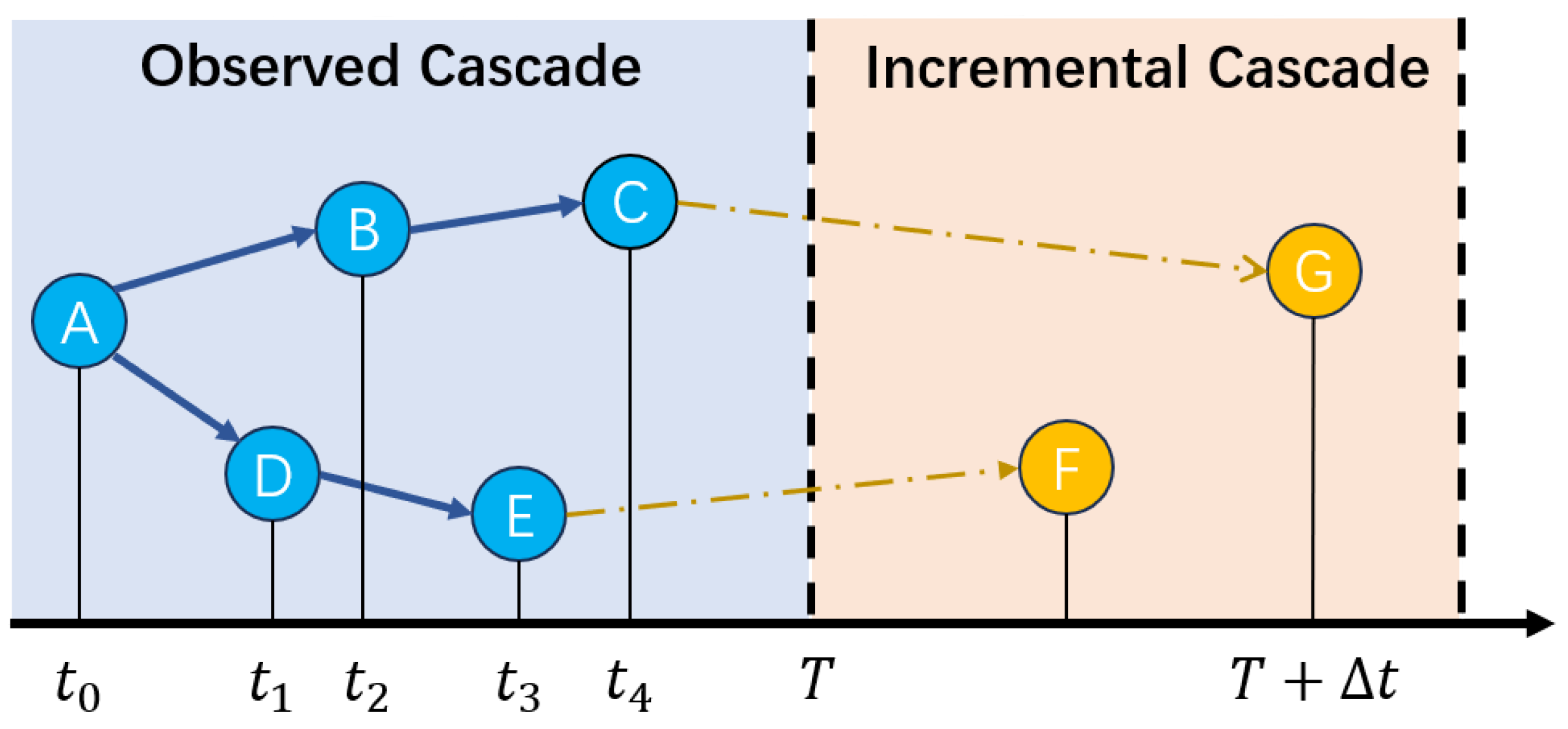
  • Cascade Graph: Suppose we have a total of M message propagation paths, denoted as M = m i ( 1 i M ) . For each message m i , we use a cascade graph g C T = ( E C T V C T ) to record the diffusion process of message m i , where V C T is a subset of nodes in V, and E C T = E V C T × V C T is the set of edges, as shown in Figure 2. A node u in V C T represents a cascade participant, such as a citation relationship in a paper citation network or a user involved in message reposting in a social network. An edge ( u , v ) V C T represents an interaction between nodes u and v.
  • Cascade Prediction: Given the information propagation processes and paths within the observation time window [0, T), our objective is to predict the incremental popularity Δ R T i between the observed popularity R T i and the final popularity R i of each cascade graph g C T . This represents the popularity of the information beyond the observation time. To avoid the inherent correlation between the final popularity and the observed popularity, we choose to predict the incremental popularity,

3.2. Proposed Model

Our cascade prediction model takes the cascade graph g C T within the observed time as input and predicts the cascade size Δ R T i outside the observed time. Our cascade prediction framework consists of the following four parts:
  • Embedding Initialization: Traverse the cascade graphs observed within the observed time, convert them into sequences, and transform the nodes in the sequences into vectors of predefined dimensions.
  • Learning micro-level features between nodes: By leveraging the inter-node self-attention mechanism, we capture the hidden features of the target node and all other nodes in the sequence at a micro-level. This allows us to update the embedding of the target node.
  • Learning meso-level features in a sequence: By utilizing multiple parallel one-dimensional convolutional layers, we obtain sequence-wide features from different dimensions at a meso-level. We then use the dynamic routing algorithm to aggregate weighted sums of sequence features from different dimensions, thereby updating the sequence features.
  • Path Encoding and Sum Pooling: Use GRU to extract the embedding relationship features between nodes in the sequence and their neighboring nodes, and sum them to obtain the features of the entire cascading graph.
  • Prediction Module: Utilize dense fully connected layers to output the predicted cascade size Δ R T i .
The above module decomposition reflects the different levels of information involved in cascade prediction. Specifically, micro-level inter-node interactions, meso-level sequence patterns, and path-level temporal dependencies exhibit distinct characteristics and are, therefore, modeled by different mechanisms. Rather than relying on a single uniform encoder, CasNS adopts specialized components(such as multi-head attention, GRU and capsule networks) at each level to capture complementary aspects of diffusion dynamics, which together form a coherent and expressive representation for cascade size prediction.

3.3. Embedding Initialization

Given a cascade graph g C T , our model first converts it into an easily processable sequential structure by traversing the entire graph using Breadth-First Search. Thus, the representation of the original g C T is a set of node sequences. For example, traversing the cascade graph g C T requires N sequences, and the longest sequence contains M nodes. We can represent the cascade graph g C T as G R N × M . Next, we use vectorized representations for each node ID. For each user’s ID, we represent it as e u ( 0 ) R D ( e i ( 0 ) R D ) , where D is the embedding dimension for each user. In this way, we can represent a sequence as Y R M × D . Thus, we can represent a cascade graph as E R N × M × D .

3.4. Learning Meso-Level Features in a Sequence

3.4.1. Positional Encoder

The key component of our proposed model is the self-attention module. Unlike RNN, the attention mechanism does not discard periodic structures. However, our model still needs to consider the positional relationships between nodes. Therefore, we incorporate position encoding on top of the initial embeddings, and the calculation is as follows:
P E ( p o s , 2 i ) = s i n ( p o s 10000 2 i d m o d e l ) ,
P E ( p o s , 2 i + 1 ) = c o s ( p o s 10000 2 i d m o d e l ) ,
where p o s refers to the position of a node in the sequence, d m o d e l represents the dimension of the node vectors, in the case of the cascade graph g C T , we have d m o d e l = D , i denotes the position of the node vector. Specifically, for each node u in the sequence, we deterministically calculate its positional encoding z ( pos ) R D . Then, U R M × D represents the positional encoding of the sequence.

3.4.2. Multi-Head Attention

After the initial encoding and position encoding, we define X = ( Y + U ) R M × D to pass through the self-attention module. Specifically, we compute the attention output S by
S = S o f t m a x Q K T M K V ,
Q = X W Q ,
K = X W K ,
V = X W V ,
here, Q, K and V are the query, key, and value matrices obtained by applying different linear transformations on the sum of the initialized embeddings and positional encodings of the sequence, denoted as X. The matrices W Q R D × M Q , W K R D × M K , W V R D × M V represent the weights for the respective linear transformations applied to X. In our experiments, the inclusion of multi-head self-attention allows for a more detailed capture of the embedding relationships between nodes. To achieve this, we use different sets of weights S 1 , S 2 , , S H to compute different self-attention outputs, denoted as W h Q , W h K , W h V h = 1 H . Finally, our output for the event sequence is given by the following:
S = S 1 , S 2 , , S H W O ,
where W O is an aggregation matrix.
The j-th column of the attention weights S o f t m a x Q K T M K represents the dependency of user u j on other nodes u i . In contrast, models based on RNN encode user node information sequentially using the hidden representation of users. This means that the state of user u j depends on the state of user u j 1 , which in turn depends on the state of user u j 2 , and so on. If any of these encodings are weak, meaning that the RNN fails to learn sufficient information related to user u k , then the hidden representation of any user u j with j k will be poorer.

3.4.3. Position-Wise Feed-Forward Networks

Afterward, the attention output S is processed through a position-wise feed-forward neural network to generate the hidden representation h ( u ) of the input user sequence:
P = R e L U S W 1 F C + b 1 W 2 F C + b 2 ,
p u j = H j , : ,
where W 1 FC R D × M H , W 2 FC R M H × D , b 1 R M H , and b 2 R D are the parameters of the neural network. Notably, W 2 FC has the same number of columns. The resulting matrix P R M × D contains the hidden representations of all user nodes in the input sequence, where each row corresponds to a user.

3.4.4. Compression Encoder

To enhance the expressive power and performance of the Multi-head Attention model and enable its training parameters to better fit nonlinear and complex functional relationships, we introduce a non-linear squashing function at the end:
S h = h 2 1 + h 2 h h .
This function normalizes the hidden representation h, which helps to stabilize the learning process in subsequent modules.

3.4.5. Gated Multi-Modal Units

In the above, we first initialize the hidden representation of the sequence nodes and then utilize self-attention mechanisms between nodes to obtain hidden embeddings of the nodes with respect to other nodes in the sequence. However, a question arises regarding how to aggregate these updated hidden representations.
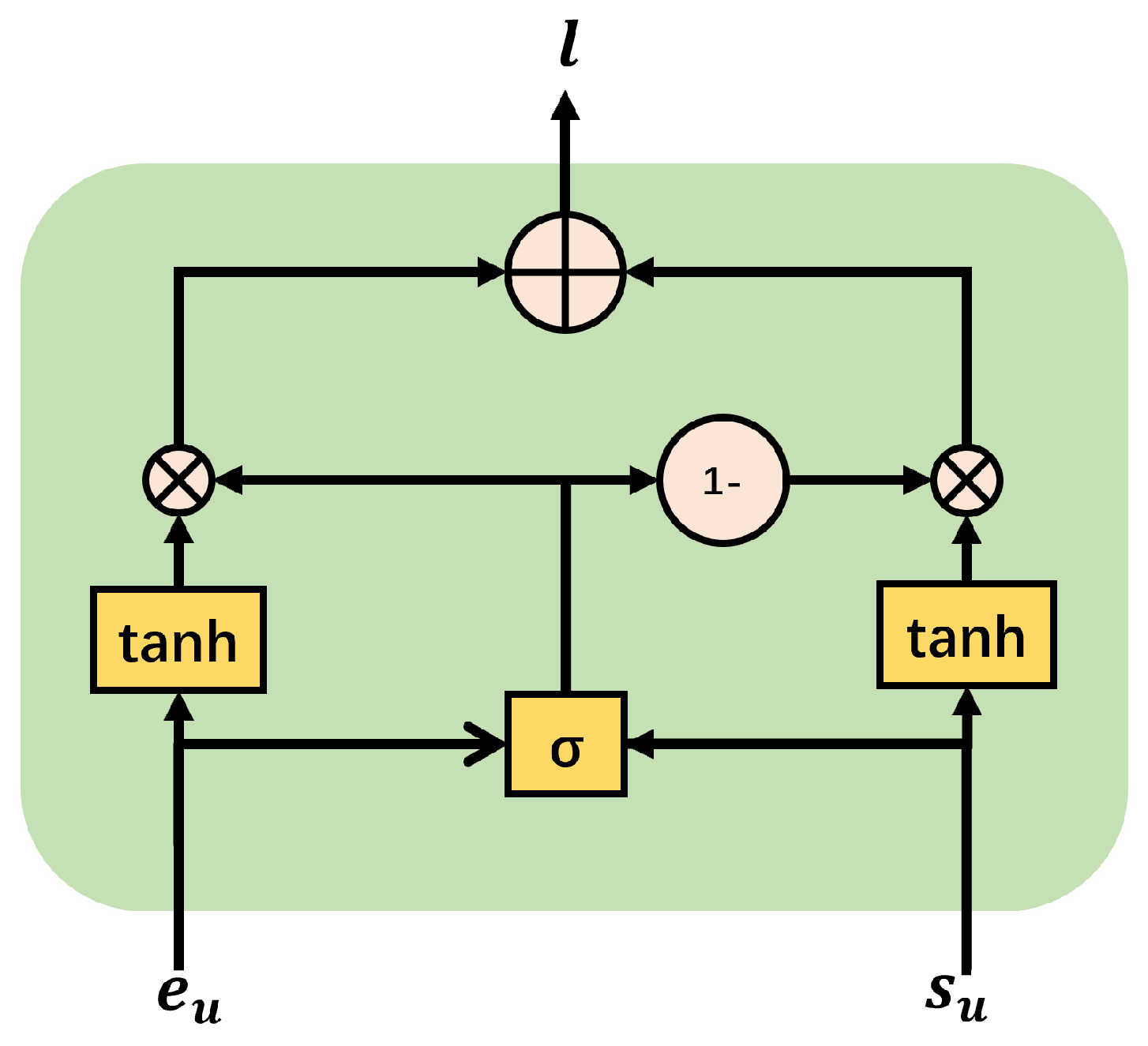
We use a gate mechanism similar to LSTM, as shown in Figure 3. It is a multimodal learning model based on gate-controlled neural networks. The Gate-Multi-modal Unit (GMU) model is designed to serve as an internal unit in neural network architectures with the purpose of finding intermediate representations based on combinations of data from different modalities. The GMU learns to use multiplication gates to determine how each modality influences the unit’s activation, and the computation is as follows:
l y = t a n h W y · Y ,
l p = t a n h W p · P ,
z = σ W Z · l y , l p ,
L = z · Y + ( 1 z ) · P ,
for any sequence l, its initialized sequence representation is denoted as Y R M × D . After updating the node features using self-attention mechanisms between nodes, the representation becomes H R M × D . The training parameters for the GMU are denoted as W y , W h , W z R . For any sequence in the cascade graph, its sequence representation through the GMU is denoted as L, and the hidden representation of node u j in the sequence is as follows:
l u j = L j , : .

3.5. Learning Micro-Level Features Between Nodes

To capture the entire sequence features, we propose a sequence-specific capsule module to overcome the limitations of previous work, which is insensitive to order (i.e., direction and position). The module consists of a horizontal convolution and a dynamic routing process. The input to the module is the initialized embedding of the sequence nodes E = [ e 1 , e 2 , , e n ] ( e i R D ) . Borrowing the idea of CNN on knowledge graphs [37], we regard the specific matrix E of sequence l as an “image” for horizontal convolution.
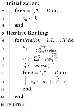
As shown in Figure 1, our module contains two 1D convolutional layers and a routing algorithm. The first 1D convolutional layer Conv1 uses ReLU as the activation function. The purpose of this layer is to transform individual node features in the sequence into local sequence features, which are then passed as input to the second 1D convolutional layer.
The second layer consists of multiple one-dimensional convolutional layers that form the primary capsules, with each convolutional layer being identical. Each convolutional layer is used to capture features of specific dimensions in the sequence. The final layer (DigitCaps) aims to fuse the obtained features from different dimensions of the sequence through a routing algorithm.
We encapsulate all elements of the same dimension into a sequence-specific capsule c l ( d ) and obtain D capsules accordingly [ c l ( d ) | d 1 , , D ]. Each capsule c l ( d ) undergoes a linear transformation via the corresponding weight matrix W c to produce a “prediction vector” c l ( d ) ^ . These vectors c l ( d ) ^ ( d 1 , , D ) are added together to generate a capsule s l . This capsule performs a nonlinear squashing function to produce vector output z l . Formally, we have the following:
z l = s q u a s h ( s l ) ,
s l = d = 1 D β d c l ( d ) ^ ,
c l ( d ) ^ = W c ( d ) c l ( d ) ,
where s q u a s h ( s l ) = s l 2 1 + s l 2 s l s l , the squashing function here is a standard component of the capsule network’s dynamic routing algorithm. While its form is identical to the one used in Section 3.4.4, its core role here is to enable the dynamic routing mechanism. β d is the coupling coefficient representing the importance of capsule c l ( d ) , which is determined by the dynamic routing process as shown in Algorithm 1.
Algorithm 1: Dynamic Routing Process
Electronics 15 00159 i001
We now obtain the hidden state z l R H of sequence l. And the embedding representation of the information propagation paths formed by N sequences is denoted as Z R N × H .

3.6. Path Encoding and Sum Pooling

After obtaining the hidden representations of the target node and other nodes in the sequence using the self-attention mechanism, we need to obtain the representation of the entire sequence at a micro-level. Here, we perform path encoding on the hidden states of nodes in the sequence and use GRU for aggregation to obtain the hidden state of the entire sequence.
To capture the evolving relationships in the information dissemination process, we employed Gated Recurrent Units (GRU), which is a specific type of Recurrent Neural Network (RNN) known for its strong performance in sequence modeling. When using GRU for modeling sequences from left to right, the representation of subsequent sequence nodes will incorporate information from previous nodes. The gate mechanism in GRU determines the proportion of new information and historical information embedded in the sequence nodes, simulating the flow of information during the diffusion process. Specifically, for the i-th node in the sequence, assuming the input node embedding l i R D and the previous hidden state h i R D as inputs, the GRU computes the updated hidden state h i = G R U ( s i , h i 1 ) , where h i R D :
u p d a t e g a t e :   u i = σ ( W u s i + U u h i 1 + b u ) ,
r e s e t g a t e :   r i = σ ( W r s i + U r h i 1 + b r ) ,
c a n d i d a t e s t a t e :   h i ˜ = t a n h ( W h s i + U h ( r i h i 1 ) + b h ) ,
h i d d e n s t a t e :   h i = u i h i ˜ + ( 1 u i ) h i 1 ,
in this context, the symbol ⊙ denotes element-wise multiplication, where W u , W r , W h , U u , U r , U h R D × D represent the matrix parameters in the GRU, and b u , b r , b h R D are the bias parameters in the GRU.
A unidirectional GRU models the sequence in a forward time order, where subsequent nodes contain progressively richer features. However, the forward nodes have little knowledge of which nodes they will influence, which does not align with the flow of information in the diffusion process. Therefore, we introduce a bidirectional GRU to address this limitation, allowing the preceding nodes to know which subsequent nodes they will propagate information to. The representation of the i-th node in the k-th sequence: h s i k R 2 D is computed using the following equations:
h s i k = h s i k h s i k ,
h s i k = G R U f ( s i , h s i + 1 k ) ,
h s i k = G R U f ( s i , h s i 1 k ) ,
where the symbol ⊕ represents the concatenation operation, h s i k and h s i k represent the forward and backward hidden vectors, respectively. The k-th sequence with length L can be denoted as [ h s 1 k , h s 2 k , , h s n k ] . Then, we take the last node’s embedding h s n k to represent the hidden state of the whole sequence. For a cascade graph with N sequences, its hidden state is as follows:
R = n = 1 N h s n k .

3.7. Prediction Module

The last part of our model consists of a multi-layer perceptron (MLP) and an adder that takes the hidden state R and P of the cascade graph as input and outputs a final prediction:
Δ R T i ^ = M L P ( R + Z ) ,
and our goal is to minimize the loss function:
l o s s = 1 K k = 1 K ( l o g ( Δ R T i ) l o g ( Δ R T i ^ ) ) 2 ,
where Δ R T i ^ is the predicted incremental popularity of cascade g C T by our model, Δ R T i is the ground-truth incremental popularity, and K is the total number of cascades. We take the logarithm of the incremental popularity because the original squared loss is prone to being influenced by outliers, while the transformed objective is similar to MAPE (Mean Absolute Percentage Error) and easier to optimize.

3.8. Framework Operational Mechanism

To concretely illustrate the execution of the CasNS framework, this section provides a detailed description of the data flow when processing a single cascade; Figure 1 also depicts the corresponding data movements during runtime.
The process begins with an original cascade graph. Using breadth-first temporal sampling, we extract N node sequences, which are subsequently padded to a uniform length M. Next, the N sequences are mapped by a shared node-embedding layer into a tensor of shape [ N , M , D ] . This initial tensor serves as the input basis for two parallel feature-extraction branches in the model.
Each of the N sequences is fed simultaneously into both branches for parallel processing. The meso-level sequence feature branch employs a capsule network: the input sequence tensor is processed by convolutions followed by the capsule network’s dynamic routing procedure to capture global, holistic characteristics of the entire sequence. The micro-level node feature branch first adds positional encodings to the input tensor and then processes the result with a multi-head self-attention-based encoder to produce context-aware node representations. A Gated Multimodal Unit (GMU) fuses the original embeddings with these context-aware embeddings to yield a refined tensor, which is finally passed into a bidirectional GRU.
After all N sequences have been processed, the model aggregates the outputs from each branch. The two aggregated vectors are concatenated and supplied to the MLP layer to produce the model’s prediction.

4. Experiment

This section conducts experiments on the two benchmark datasets introduced and compares with state-of-the-art baseline models for cascade prediction to evaluate our model. Ablation experiments are also carried out to analyze the contributions of different modules in our model.

4.1. Dataset

We apply our proposed model to two different cascade prediction scenarios to evaluate its performance. The first scenario predicts retweet cascades on Sina Weibo, and the second scenario predicts tweet propagation cascades on Twitter. Table 1 lists the statistical information of the datasets.
Sina Weibo: This dataset collected and provided by Cao et al. [3] can be openly accessed on their website. This dataset includes Weibo messages with more than 10 retweets, which were posted on 1 June 2016, along with the retweets received within 24 h of the original post. In addition to user IDs, the retweet information includes the retweet path and the time of retweeting. We consider cascades that were posted between 8:00 and 18:00 and have less than 1000 retweets as candidates for generating the global network structure, denoted as G. To validate our model’s ability to achieve high performance with a small training set, we randomly select over 1000 cascades that meet the aforementioned criteria. The specific number of cascades depends on the observation time. Next, the dataset is divided into training, validation, and testing sets based on the chronological order of message publication. Specifically, the first 70% of the data are used as the training set, the middle 15% are used as the validation set, and the remaining 15% are used as the testing set. The observation time length, denoted as T, is set to 1, 2, or 3 h, respectively.
Twitter: This dataset, collected by Weng et al. [38] includes publicly available English-written tweets posted between 24 March and 25 April 2012. We consider topic hashtags and their adopters as independent information diffusion processes. The global graph of the Twitter dataset is constructed using various relationships, including mutual followings/followers between users, retweeted tweets, and mention interactions. The cascade graph is built based on these three relationships. To validate our model’s performance on large-scale data, we select all cascades that meet the requirements. The observation time length, denoted as T, is set to 1 or 2 days, respectively.

4.2. Baseline Methods

To validate that our model has strong predictive performance on real-world datasets, we also experimented with other advanced methods on the two datasets, but these other methods were not able to simultaneously capture the Node-level and Sequence-level features of the sequences.
Feature-Linear is the most widely used information diffusion prediction model. These models typically involve manual feature extraction from the data, followed by training and evaluation using machine learning models. For instance, Szabo and Huberman [39] used observed popularity, denoted as P j ( t o ) , to predict the predicted popularity, denoted as P j ( t p ) ^ , of news articles and online videos. They utilized observed popularity and cumulative popularity as features. These features were then fed into linear regression and MLP models to predict the popularity.
DeepCas [2] is the first model that truly applies deep learning to cascade prediction. Its primary goal is to predict the future popularity of information by analyzing the paths of information propagation. Specifically, it first processes the cascade graphs into multiple sequences, then uses recurrent neural networks to obtain embeddings of the sequences, and finally obtains the embedding of the cascade graph by weighted summing of all sequences. However, its weighted summing is based only on mathematical assumptions rather than the actual structure of cascade graphs.
DeepHawkes [3]. A model is proposed based on DeepCas by adding Hawkes processes [40]. It replaces the weighted summing of sequences in DeepCas based on mathematical assumptions with weight summing based on cascade diffusion times, which is closer to reality and enhances the interpretability of the model.
CasCN [4] is a model similar in concept to DeepHawkes, as they are both built based on self-exciting processes. CasCN introduces graph convolutional neural networks (GCNs) on top of DeepHawkes to directly aggregate node features in the graph and obtain global features of the graph. However, due to the varying number of nodes in different information cascades, the constructed Laplacian matrix has different dimensions. This constraint limits CasCN to only use cascade graphs with observed node counts ranging from 10 to 1000 in their experiments. This requirement for dataset selection is quite strict, and our model aims to avoid such limitations.
GTGCN [5] is a graph-based time-aware information learning framework that builds upon an enhanced graph convolutional network (GCN). It combines GCN with a recurrent neural network (RNN) in a linear fashion and introduces time parameters to capture temporal information governing information propagation within snapshots, as well as inherent temporal dependencies between different snapshots.
CasFlow [41] is a cascade prediction framework that obtains high-quality node embeddings by learning the latent representations of cascade graph structural information and cascade diffusion time information. Additionally, CasFlow can capture the uncertainty in information propagation and realize hierarchical learning of information diffusion patterns by doing so.
CasHAN [42] builds upon DeepCas and incorporates node-level self-attention mechanisms and community detection to capture meso-scale features in information propagation, while removing redundant nodes during the cascade prediction process.
The selected baselines cover representative paradigms ranging from traditional feature-engineering methods to modern deep learning approaches. Feature-Linear represents classical feature-based methods and serves as a reference for highlighting the overall advantages of deep learning. DeepCas [2] and DeepHawkes [3] are pioneering RNN-based models that focus on sequential modelling of propagation paths, enabling a comparison with our model in terms of sequence-level feature capture. CasCN [4] operates directly on graph structures and provides a key baseline for node-level feature modeling. GTGCN [5] and CasFlow [41] adopt hybrid strategies that integrate graph topology with temporal dynamics, reflecting an important research direction. CasHAN [42] incorporates attention mechanisms and constitutes the most direct comparison to our node-level self-attention module. Overall, these baselines ensure both the relevance and diversity of the experimental comparison.

4.3. Experimental Setup

We will measure the performance of each model using both mean squared error (MSE) and mean absolute percentage error (MAPE).
MSE is a widely used regression evaluation metric in the cascade prediction domain. Let y k and y k ^ represent the true value Δ R T k and predicted value Δ R T k ^ logarithm, respectively, for the k-th cascade. Then, the calculation formula for MSE is as follows:
M S E = 1 K i = 1 K y i y i ^ 2 ,
where K represents the total number of cascades, y k = l o g ( Δ R T k ) , y k ^ = l o g ( Δ R T k ^ ) , and the lower the final MSE result, the better the model performance.
MAPE is used to measure the mean absolute percentage error between predicted values and actual values. It can reflect the percentage relationship between the prediction error and the actual value. Moreover, MAPE ignores the positive and negative nature of errors, directly examines the absolute value of errors, and can more objectively reflect predictive accuracy. The calculation formula of MAPE is as follows:
M A P E = 1 K i = 1 K y i y i ^ y i .
For model parameters, the number of units per GRU hidden layer is 64, the initial learning rate for user embeddings and other variables is 0.0003, and the Adam optimizer is used for iterations. According to the DeepCas setting, the size of user embeddings is set to 50, the number of fully connected layers is 2, and the dimensions of the hidden layers are 64 and 32, respectively. The number of Transformer encoder layers is set to 2, and the number of heads is set to 4. N is the total number of sequences traversed in a cascade graph and M is the maximum sequence length in the traversal of the cascade graph, for the Sina Weibo dataset, if the observation time is 1 h, then M = 9 , if the observation time is 2 h and 3 h, then M = 10; for the twitter dataset, the observation time is 1 day or 2 days, M = 10 .

4.4. Performance Comparison

The overall predictive performance of all competitive methods on two different datasets is shown in Table 2. Our proposed model shows better loss than other baseline methods on all datasets. For example, on the Sina Weibo dataset, when the observation time T = 1 h , the MSE predictive error of our model is 2.216, while the other seven methods increase by 0.071, 0.073, 0.205, 0.700, 1.122, 1.252, and 1.439, respectively. Among the seven methods mentioned above, Feature-linear exhibits the worst performance. This is because the predictive power of this model relies on the quality of handcrafted features, which require expertise from multiple domains. However, the design of these features often fails to effectively integrate with cascade graphs, greatly limiting their performance.
DeepCas introduced deep learning for cascade prediction, leading to significant performance improvements compared to traditional machine learning methods. The main reason for this improvement is that deep learning methods can autonomously learn feature representations of cascade graphs, eliminating the cumbersome process of manual feature extraction. However, due to its approach of aggregating sequence features into cascade features, its performance is still inferior to other deep learning-based methods. DeepHawkes integrates models based on self-exciting point processes, proposes improvements to the deficiencies of DeepCas, introduces time weight parameters, and improves predictive performance while increasing the interpretability of deep learning models. However, since the model can only obtain the embedding relation of neighboring nodes, the model’s performance cannot be qualitatively improved relative to DeepCas.
For the two advanced methods, GTGCN and CasFlow, their predictive errors on the two datasets are relatively close to each other and lower than the above four methods. Compared with DeepHawkes, GTGCN’s focus is on capturing the temporal evolution information within a snapshot and the dependencies between discrete graph sequences in the information diffusion process, which also improves predictive performance. The focus of CasFlow lies in obtaining high-quality initial embeddings for nodes. However, the predictive errors of GTGCN and CasFlow are still at least 9.2% and 3.2% higher than our model in MSE metrics. Compared with GTGCN and CasFlow, our model learns effective local cascade graph structure representations, obtaining high-quality node embeddings and embedding relationships with other nodes in the cascade graph, rather than learning complex global propagation graphs or high-quality node features, thus providing a greater contribution to cascade prediction.
For the state-of-the-art model CasHAN, our model still outperforms it on various datasets. Although CasHAN introduces community detection and inter-node self-attention mechanisms compared with other baseline models, to some extent, eliminating the influence of redundant nodes during the prediction process, it fails to capture the complete hidden relationships between the target node and all nodes in the sequence due to the use of dot product-based softmax for obtaining inter-node embeddings. However, our model improves upon this by simultaneously capturing the comprehensive hidden relationships between the target node and all nodes in the sequence using Query, Key, and Value, resulting in updated node embeddings that contain richer and more important information.
CasNS comprehensively considers the feature relationships between nodes and the features of the entire graph. The results shown in Table 2 prove the effectiveness of the proposed model. In addition, our model performs relatively well when using different observation times T. The larger the observation time T, the lower the MSE, and the easier the cascade prediction. After all, the size of a cascade graph is finite. The longer the observation time, the more cascade graph information is obtained, which is more conducive to predicting the popularity of information spread. In addition, we also found that when the observation time is small, our model can perform much better than other models, which proves that our model has very strong predictive power for incomplete cascades.
When comparing our experimental results on two real datasets, the error on the Twitter dataset is noticeably higher than the error on the Sina Weibo dataset. The specific reason is that compared with the Sina Weibo dataset, the Twitter dataset does not have originating nodes; in other words, the cascade graphs in the Twitter dataset only capture part of the path of information propagation, resulting in incompleteness of cascade graphs and increasing unpredictability, making predicting cascade increments more complex.

4.5. Ablation Study

Here are two variants of CasNS are proposed to prove the effectiveness of the two main components of CasNS:
CasNS-node: The model includes a node-level attention mechanism based on user influence but does not directly extract sequence features across different dimensions. It only utilizes the node embedding of the last GRU to represent the embedding of the entire sequence.
CasNS-sequence: The model directly captures sequence features at a meso-level across different dimensions. It removes the usage of the node-level self-attention mechanism at a micro-level to capture relationships between nodes.
Table 2 shows the predictive performance of these two CasNS variants. The loss of CasNS-node is lower than the loss of CasNS-sequence, indicating that the importance of node features in cascade prediction is relatively higher than that of sequence features. However, both models have lower losses compared with most of the baseline models, but higher than CasNS. This suggests that both node features and sequence features are essential in cascade prediction, and they complement each other. The ablation study demonstrates the interpretability of our model in capturing both the node features and sequence features of the cascade graph simultaneously.

4.6. Analysis of Sensitivity to Hyper-Parameters

4.6.1. The Number of Heads in the Multi-Head Attention Models

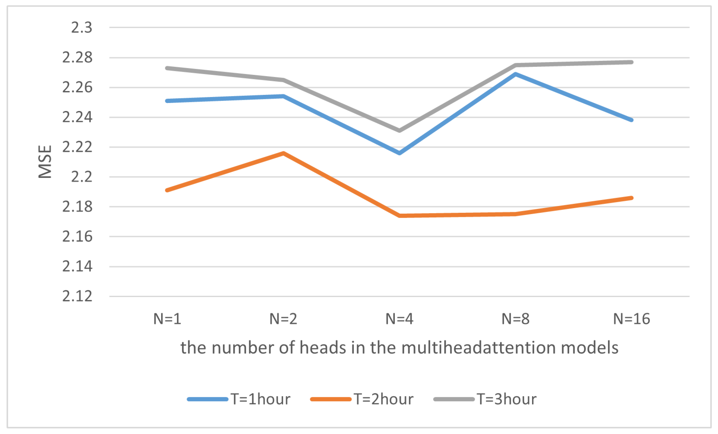
The number of heads in the learning meso-level features module to the number of attention heads used in the multi-head self-attention mechanism. To verify the impact of the number of heads in the multi-head attention models on model performance, we use the Sina Weibo dataset, set the observation time to 1, 2, and 3 h, set the number of units per GRU hidden layer to 64, the initial learning rate for user embeddings and other variables is 0.0003, and Adam optimizer is used for iterations, the size of user embeddings is set to 50, the number of fully connected layers is 2, the dimensions of the hidden layers are 64 and 32, respectively. The number of Transformer encoder layers is set to 1, and the number of heads N in the multi-head attention models must be divisible by the embedding dimension, so it is separately set to 1, 2, 4, 8, and 16.
Figure 4 shows the performance when N is 1, 2, 4, 8, and 16 on the Sina Weibo dataset. We can find that when N is not more than 4, increasing the number of heads can improve the model’s performance. For tasks that model text sequences, increasing the number of heads may achieve better results. More heads allow the model to pay better attention to different parts of the input sequence, improving the model’s representation and generalization abilities.
However, increasing the number of heads also increases the computational complexity and number of parameters of the model, thereby reducing the training and inference efficiency of the model, and increasing training time and computational cost. Therefore, when N equals 8, the performance will decrease instead. So a balance needs to be struck between computational resources and efficiency.

4.6.2. The Number of Sub-Encoder-Layers in the Encoder

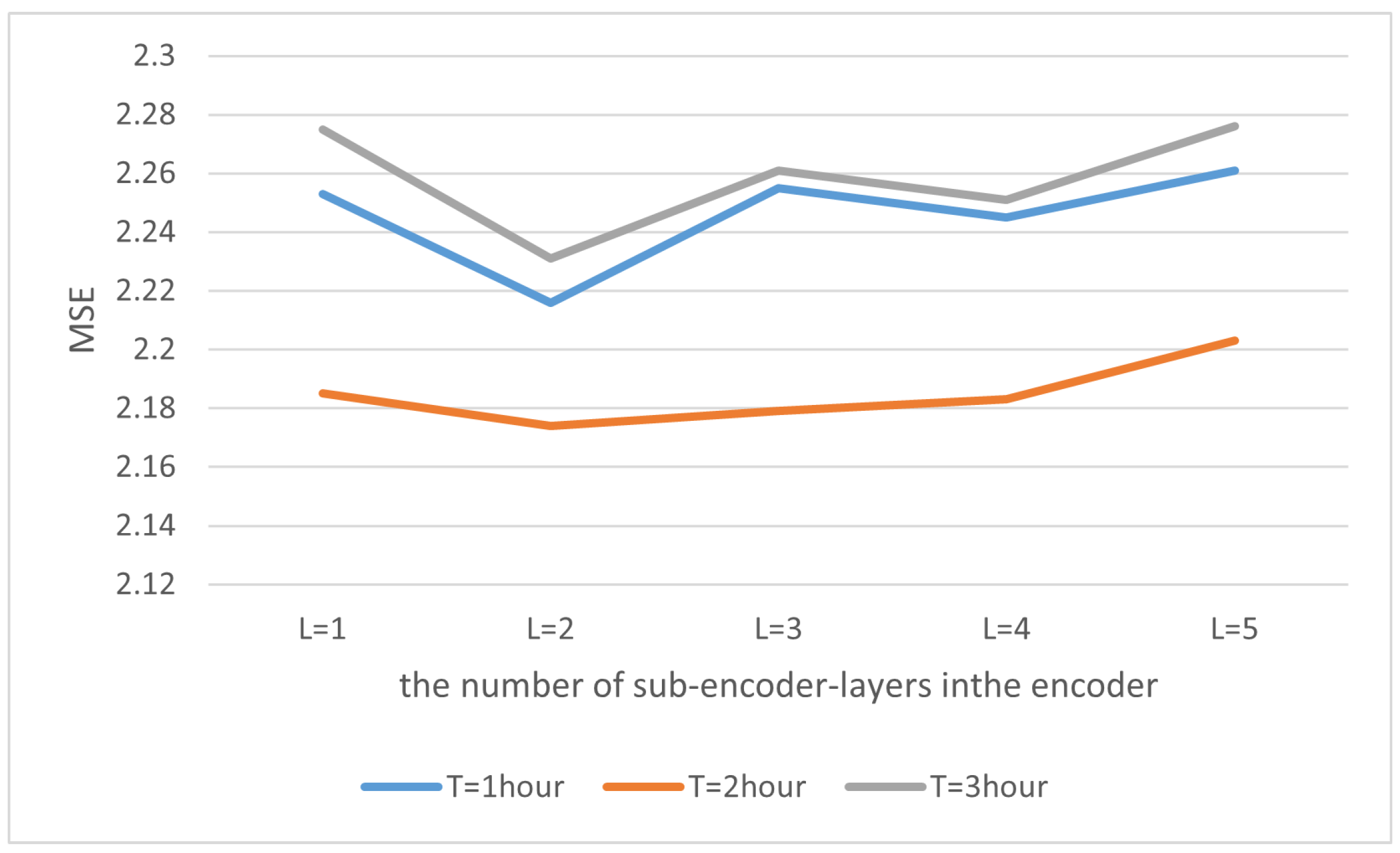
The number of layers in the Learning meso-level features module refers to the deep neural network formed by stacking multiple self-attention layers and feed-forward neural network layers together. To verify the impact of the number of sub-encoder layers in the encoder on model performance, we still use the Sina Weibo dataset, keeping the other hyper-parameters unchanged, setting the number of heads N to 4, and the number of encoder layers to 1, 2, 3, 4 and 5, respectively.
Figure 5 shows the performance when num-encoder-layers are 1, 2, 3, 4, and 5 on the Sina Weibo dataset. We can find that for the same observation time, the performance is best when the number of layers is 2.
In theory, increasing the number of encoder layers can enhance the model’s expression ability and improve model performance within a certain range by repeatedly convolving the entire sequence information, thereby continuously improving model performance. However, in practice, the improvement becomes smaller and smaller with the increase in layers. This is because, for time series data, the number of layers is sufficient to make the contained historical content rich enough. Additional layers have limited returns, and too many layers will make model training more difficult, increase computational costs, and parameter convergence issues. This is because gradients propagate through too many layers, making it easy for gradients to diffuse or vanish.

4.7. Computational Complexity and Scalability

To provide a comprehensive evaluation of our proposed architecture, we address its computational complexity and scalability. For a concrete, quantitative perspective, we analyzed the model’s performance on our experimental setup, which consists of an Intel Core i5-13600KF CPU, 32 GB of RAM, and an NVIDIA RTX 3090 GPU (24 GB GDDR6X VRAM). The estimated performance metrics are summarized and compared against a lightweight baseline such as DeepCas in Table 3.
As the Table 3 illustrates, CasNS has approximately four times the parameters and requires 3–4 times longer training time per epoch compared to DeepCas. This is an expected outcome, as the model’s overall complexity is dominated by the Transformer’s self-attention mechanism, which has a complexity of O ( L 2 · d ) . In contrast, the Capsule Network and GRU components, similar to the baseline, operate with a complexity that is linear with respect to the sequence length L.
This complexity profile represents a deliberate design trade-off, reflected in higher training and inference times. However, this is justified by a 3.5% increase in performance. We contend that this increase in computational time is an acceptable trade-off for the superior performance achieved. This higher computational cost is intentionally accepted to leverage the synergistic strengths of our hybrid model, which uniquely captures long-range dependencies, hierarchical features, and temporal dynamics. As supported by our experiments, the significant and consistent reduction in MSE validates this approach, demonstrating a meaningful improvement that justifies the additional computational investment in application contexts where accuracy is critical.
Moreover, it is noteworthy that the single-cascade inference latency remains in the millisecond range (approx. 15–20 ms), indicating its viability for near-real-time or offline prediction tasks. Nevertheless, we acknowledge that the quadratic complexity poses a scalability challenge for extremely long sequences. For practical large-scale deployment, this can be managed by applying sequence truncation to a feasible length L max , a common practice we adopted in our experiments. Furthermore, a promising direction for future work is to integrate more efficient Transformer variants, such as those with linear complexity, which would substantially enhance scalability while preserving the core architectural benefits.

5. Conclusions

This paper proposes a framework called CasNS (Node-level and Sequence-level Features for Cascade Prediction) for predicting the future popularity of messages in social networks. We consider the information propagation paths in social networks as a directed graph, and our model effectively captures the micro-level node features, meso-level sequence features, and macro-level graph features in the directed graph. Experimental results on various real-world datasets demonstrate that all these features are essential for accurate information propagation prediction, and our model achieves state-of-the-art accuracy while effectively capturing these features. Furthermore, our model is highly scalable and can analyze more complex data. In future work, we will explore methods that can simultaneously capture node features, sequence features, and graph features more comprehensively. We aim to reduce the algorithm complexity and time complexity while ensuring accurate feature capturing.

Practical Implications and Future Work

In recent years, with the rapid proliferation of digital services and online communities, social network security has emerged as a paramount global challenge. Against this backdrop, the ability to accurately predict and effectively manage the dynamics of information propagation is crucial for maintaining the safety and stability of cyberspace.
The CasNS framework proposed in this paper offers a novel approach to addressing this challenge. Its core practical value lies in its strong performance in early-stage cascade prediction. The early and reliable identification of cascade growth trends is critical for a range of time-sensitive applications. Its most vital application is in the domain of social network security, where it can serve as a powerful tool for the proactive detection and mitigation of harmful misinformation, online rumors, and malicious content, thereby providing platform administrators and regulators with a valuable window for timely intervention. Moreover, the framework demonstrates significant potential in other areas, such as optimizing budget allocation in digital marketing and guiding public communication during public health emergencies. Technically, by providing reliable early predictions, CasNS offers decision-makers a critical opportunity for proactive intervention. The framework’s architecture is also designed with scalability in mind, allowing it to be extended to accommodate more complex propagation data and heterogeneous network structures.
Looking ahead, our future work will proceed along two primary avenues. First, we plan to further enhance the modeling of multi-level heterogeneous features within the CasNS framework to capture more nuanced propagation dynamics. Second, we will explore more efficient model architectures to significantly reduce computational and time complexity. Collectively, these efforts will aim to facilitate the effective deployment and application of CasNS in large-scale, real-world systems.

Author Contributions

Conceptualization, G.L. and N.Z.; methodology, G.L., Y.G. and X.C.; validation, G.L., X.C., Y.G. and N.Z.; formal analysis, X.C.; investigation, N.Z.; writing—original draft preparation, G.L.; writing—review and editing, X.C. and Y.G.; supervision, N.Z. All authors have read and agreed to the published version of the manuscript.

Funding

This research was funded in part by the National Natural Science Foundation of China (62341112), in part by the Shaanxi Provincial Key Research and Development Program (2023-ZDLGY-51).

Data Availability Statement

Data are contained within the article.

Conflicts of Interest

The authors declare no conflicts of interest.

References

  1. Bouarara, H.A. Recurrent Neural Network (RNN) to Analyse Mental Behaviour in Social Media. Int. J. Softw. Sci. Comput. Intell. 2021, 13, 1–11. [Google Scholar] [CrossRef]
  2. Li, C.; Ma, J.; Guo, X.; Mei, Q. DeepCas: An End-to-end Predictor of Information Cascades. In Proceedings of the 26th International Conference on World Wide Web (WWW ’17), Perth, Australia, 3–7 April 2017; pp. 577–586. [Google Scholar] [CrossRef]
  3. Cao, Q.; Shen, H.; Cen, K.; Ouyang, W.; Cheng, X. DeepHawkes: Bridging the Gap between Prediction and Understanding of Information Cascades. In Proceedings of the 2017 ACM on Conference on Information and Knowledge Management (CIKM ’17), Singapore, 6–10 November 2017; pp. 1149–1158. [Google Scholar] [CrossRef]
  4. Chen, X.; Zhou, F.; Zhang, K.; Trajcevski, G.; Zhong, T.; Zhang, F. Information Diffusion Prediction via Recurrent Cascades Convolution. In Proceedings of the 2019 IEEE 35th International Conference on Data Engineering (ICDE), Macao, China, 8–11 April 2019; pp. 770–781. [Google Scholar] [CrossRef]
  5. Yang, C.; Bao, P.; Yan, R.; Li, J.; Li, X. A Graph Temporal Information Learning Framework for Popularity Prediction. In Proceedings of the Companion Proceedings of the Web Conference 2022 (WWW ’22), Lyon, France, 25–29 April 2022; pp. 239–242. [Google Scholar] [CrossRef]
  6. Shen, H.; Wang, D.; Song, C.; Barabási, A. Modeling and Predicting Popularity Dynamics via Reinforced Poisson Processes. In Proceedings of the AAAI Conference on Artificial Intelligence, Québec City, QC, Canada, 27–31 July 2014. [Google Scholar]
  7. Lu, Y.; Yu, L.; Zhang, T.; Zang, C.; Cui, P.; Song, C.; Zhu, W. Collective Human Behavior in Cascading System: Discovery, Modeling and Applications. In Proceedings of the 2018 IEEE International Conference on Data Mining (ICDM), Singapore, 17–20 November 2018; pp. 297–306. [Google Scholar] [CrossRef]
  8. Sreenivasan, S.; Chan, K.S.; Swami, A.; Korniss, G.; Szymanski, B.K. Information Cascades in Feed-Based Networks of Users with Limited Attention. IEEE Trans. Netw. Sci. Eng. 2017, 4, 120–128. [Google Scholar] [CrossRef]
  9. Li, Q.; Wu, Z.; Yi, L.; K.S., N.; Qu, H.; Ma, X. WeSeer: Visual Analysis for Better Information Cascade Prediction of WeChat Articles. IEEE Trans. Vis. Comput. Graph. 2020, 26, 1399–1412. [Google Scholar] [CrossRef] [PubMed]
  10. Kong, Q.; Rizoiu, M.A.; Xie, L. Modeling Information Cascades with Self-exciting Processes via Generalized Epidemic Models. In Proceedings of the 13th International Conference on Web Search and Data Mining (WSDM ’20), Houston, TX, USA, 3–7 February 2020; pp. 286–294. [Google Scholar] [CrossRef]
  11. Zhu, L.; Zheng, T. Pattern dynamics analysis and application of west nile virus spatiotemporal models based on higher-order network topology. Bull. Math. Biol. 2025, 87, 121. [Google Scholar] [CrossRef]
  12. Zhu, L.; Ding, Y.; Shen, S. Green behavior propagation analysis based on statistical theory and intelligent algorithm in data-driven environment. Math. Biosci. 2025, 379, 109340. [Google Scholar] [CrossRef] [PubMed]
  13. Li, Q.; Hu, B.; Xu, W.; Xiao, Y. A group behavior prediction model based on sparse representation and complex message interactions. Inf. Sci. 2022, 601, 224–241. [Google Scholar] [CrossRef]
  14. Wang, Y.; Wang, J.; Wang, H.; Zhang, R.; Li, M. Users’ mobility enhances information diffusion in online social networks. Inf. Sci. 2021, 546, 329–348. [Google Scholar] [CrossRef]
  15. Chen, X.; Zhou, X.; Chan, J.; Chen, L.; Sellis, T.; Zhang, Y. Event Popularity Prediction Using Influential Hashtags From Social Media. IEEE Trans. Knowl. Data Eng. 2022, 34, 4797–4811. [Google Scholar] [CrossRef]
  16. Tian, X.; Qiu, L.; Zhang, J. User behavior prediction via heterogeneous information in social networks. Inf. Sci. 2021, 581, 637–654. [Google Scholar] [CrossRef]
  17. Wang, K.; Wang, P.; Chen, X.; Huang, Q.; Mao, Z.; Zhang, Y. A Feature Generalization Framework for Social Media Popularity Prediction. In Proceedings of the 28th ACM International Conference on Multimedia (MM ’20), Seattle, WA, USA, 12–16 October 2020; pp. 4570–4574. [Google Scholar] [CrossRef]
  18. Alweshah, M.; Khalaileh, S.A.; Gupta, B.B.; Almomani, A.; Hammouri, A.I.; Al-betar, M.A. The monarch butterfly optimization algorithm for solving feature selection problems. Neural Comput. Appl. 2020, 34, 11267–11281. [Google Scholar] [CrossRef]
  19. Zhao, T.; Liu, Y.; Neves, L.; Woodford, O.; Jiang, M.; Shah, N. Data augmentation for graph neural networks. In Proceedings of the AAAI Conference on Artificial Intelligence, Virtually, 2–9 February 2021; Volume 35, pp. 11015–11023. [Google Scholar]
  20. Xiao, C.; Liu, C.; Ma, Y.; Li, Z.; Luo, X. Time sensitivity-based popularity prediction for online promotion on Twitter. Inf. Sci. 2020, 525, 82–92. [Google Scholar] [CrossRef]
  21. Carta, S.M.; Podda, A.S.; Recupero, D.R.; Saia, R.; Usai, G. Popularity Prediction of Instagram Posts. Information 2020, 11, 453. [Google Scholar] [CrossRef]
  22. Liao, D.; Xu, J.; Li, G.; Huang, W.; Liu, W.; Li, J. Popularity Prediction on Online Articles with Deep Fusion of Temporal Process and Content Features. In Proceedings of the AAAI Conference on Artificial Intelligence, Honolulu, HI, USA, 27 January–1 February 2019. [Google Scholar]
  23. Liu, Y.; Bao, Z.; Zhang, Z.; Tang, D.; Xiong, F. Information cascades prediction with attention neural network. Hum.-Centric Comput. Inf. Sci. 2020, 10, 13. [Google Scholar] [CrossRef]
  24. Shang, J.; Huang, S.; Zhang, D.; Peng, Z.J.; Liu, D.; Li, Y.; Xu, L. RNe2Vec: Information diffusion popularity prediction based on repost network embedding. Computing 2020, 103, 271–289. [Google Scholar] [CrossRef]
  25. Tang, S.; Li, Q.; Ma, X.; Gao, C.; Wang, D.; Jiang, Y.; Ma, Q.; Zhang, A.; Chen, H. Knowledge-based Temporal Fusion Network for Interpretable Online Video Popularity Prediction. In Proceedings of the ACM Web Conference 2022 (WWW ’22), Lyon, France, 25–29 April 2022; pp. 2879–2887. [Google Scholar] [CrossRef]
  26. Xu, K.; Lin, Z.; Zhao, J.; Shi, P.; Deng, W.; Wang, H. Multimodal Deep Learning for Social Media Popularity Prediction with Attention Mechanism. In Proceedings of the 28th ACM International Conference on Multimedia (MM ’20), Seattle, WA, USA, 12–16 October 2020; pp. 4580–4584. [Google Scholar] [CrossRef]
  27. Zhang, Y.; Liu, J.; Guo, B.; Wang, Z.; Liang, Y.; Yu, Z. App Popularity Prediction by Incorporating Time-Varying Hierarchical Interactions. IEEE Trans. Mob. Comput. 2022, 21, 1566–1579. [Google Scholar] [CrossRef]
  28. Vaswani, A.; Shazeer, N.; Parmar, N.; Uszkoreit, J.; Jones, L.; Gomez, A.N.; Kaiser, L.; Polosukhin, I. Attention is all you need. In Proceedings of the 31st International Conference on Neural Information Processing Systems (NIPS’17), Long Beach, CA, USA, 4–9 December 2017; pp. 6000–6010. [Google Scholar]
  29. Dai, Z.; Yang, Z.; Yang, Y.; Carbonell, J.; Le, Q.V.; Salakhutdinov, R. Transformer-XL: Attentive Language Models Beyond a Fixed-Length Context. arXiv 2019, arXiv:1901.02860. [Google Scholar]
  30. Wang, C.; Li, M.; Smola, A.J. Language Models with Transformers. arXiv 2019, arXiv:1904.09408. [Google Scholar] [PubMed]
  31. Zuo, S.; Jiang, H.; Li, Z.; Zhao, T.; Zha, H. Transformer Hawkes Process. In Proceedings of the 37th International Conference on Machine Learning, Virtual, 13–18 July 2020; Volume 119, pp. 11692–11702. [Google Scholar]
  32. Zhou, H.; Zhang, S.; Peng, J.; Zhang, S.; Li, J.; Xiong, H.; Zhang, W. Informer: Beyond Efficient Transformer for Long Sequence Time-Series Forecasting. arXiv 2020, arXiv:2012.07436. [Google Scholar] [CrossRef]
  33. Sabour, S.; Frosst, N.; Hinton, G.E. Dynamic routing between capsules. In Proceedings of the 31st International Conference on Neural Information Processing Systems (NIPS’17), Long Beach, CA, USA, 4–9 December 2017; pp. 3859–3869. [Google Scholar]
  34. Jayasekara, H.; Jayasundara, V.; Athif, M.; Rajasegaran, J.; Jayasekara, S.; Seneviratne, S.; Rodrigo, R. TimeCaps: Capturing Time Series Data With Capsule Networks. arXiv 2022, arXiv:1911.11800. [Google Scholar] [CrossRef]
  35. Elhalwagy, A.; Kalganova, T. Multi-Channel LSTM-Capsule Autoencoder Network for Anomaly Detection on Multivariate Data. Appl. Sci. 2022, 12, 11393. [Google Scholar] [CrossRef]
  36. Wu, B.; He, X.; Zhang, Q.; Wang, M.; Ye, Y. GCRec: Graph-Augmented Capsule Network for Next-Item Recommendation. IEEE Trans. Neural Netw. Learn. Syst. 2023, 34, 10164–10177. [Google Scholar] [CrossRef]
  37. Dettmers, T.; Minervini, P.; Stenetorp, P.; Riedel, S. Convolutional 2D Knowledge Graph Embeddings. arXiv 2018, arXiv:1707.01476. [Google Scholar] [CrossRef]
  38. Weng, L.; Menczer, F.; Ahn, Y.Y. Virality Prediction and Community Structure in Social Networks. Sci. Rep. 2013, 3, 2522. [Google Scholar] [CrossRef] [PubMed]
  39. Szabo, G.; Huberman, B.A. Predicting the popularity of online content. Commun. ACM 2010, 53, 80–88. [Google Scholar] [CrossRef]
  40. Weiss, E.A. Association for computing machinery (ACM). In Encyclopedia of Computer Science; John Wiley and Sons Ltd.: Hoboken, NJ, USA, 2003; pp. 103–104. [Google Scholar]
  41. Xu, X.; Zhou, F.; Zhang, K.; Liu, S.; Trajcevski, G. CasFlow: Exploring Hierarchical Structures and Propagation Uncertainty for Cascade Prediction. IEEE Trans. Knowl. Data Eng. 2023, 35, 3484–3499. [Google Scholar] [CrossRef]
  42. Zhong, C.; Xiong, F.; Pan, S.; Wang, L.; Xiong, X. Hierarchical attention neural network for information cascade prediction. Inf. Sci. 2023, 622, 1109–1127. [Google Scholar] [CrossRef]
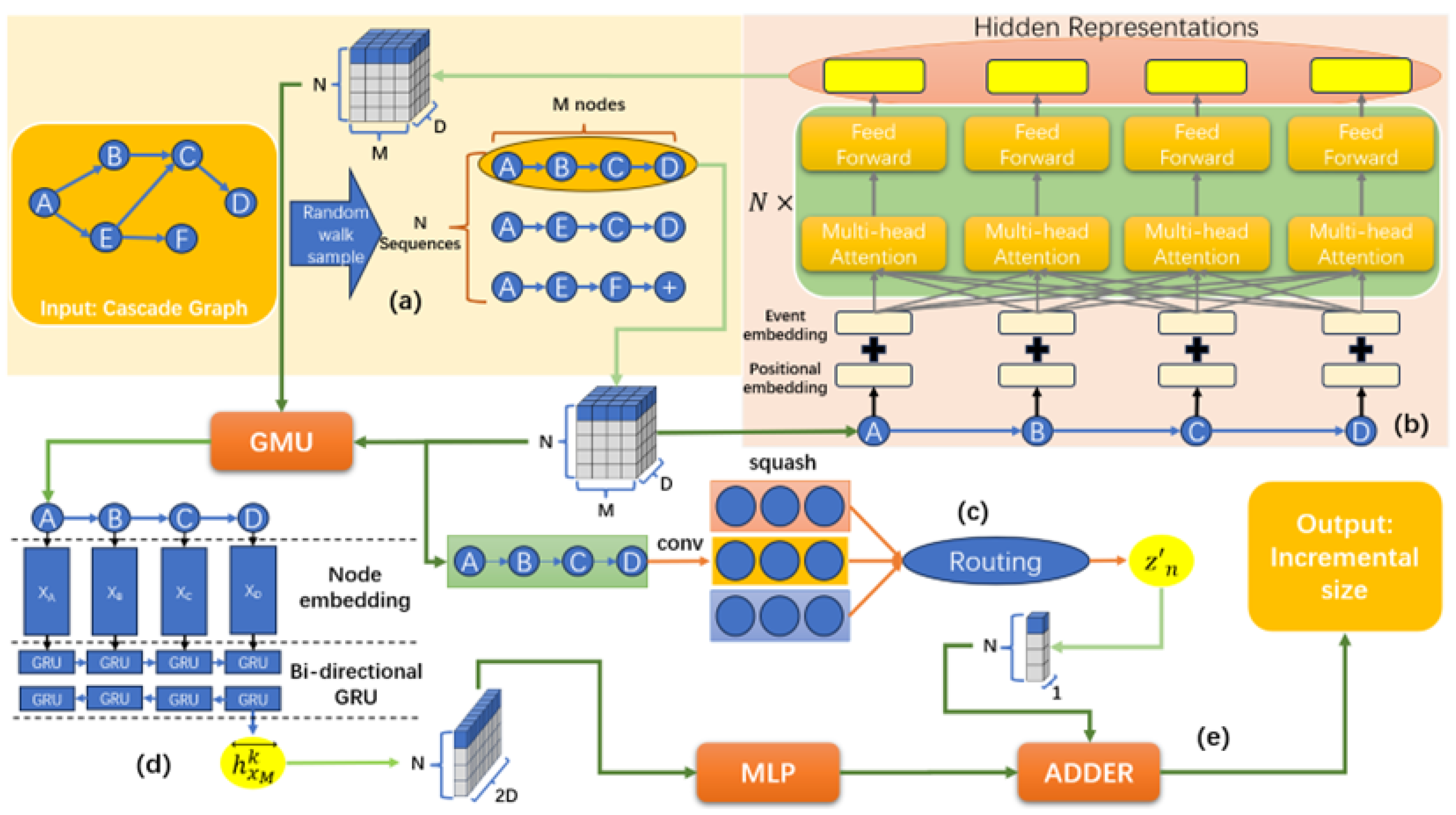
Figure 1. Overall framework of the proposed CasNS model. The model comprises four key components: (a) Embedding Initialization (b) learning micro-level features between nodes (c) learning meso-level features in a sequence (d) path encoding and sum pooling (e) prediction module. A–F are user nodes in the cascade graph.
Electronics 15 00159 g001
Figure 2. An example of a cascading incremental prediction problem. A is the originator of the information cascade. A–G are user nodes in the cascade graph.
Electronics 15 00159 g002
Figure 3. Gated multi-modal units.
Electronics 15 00159 g003
Figure 4. The impact of the number of heads in the multi-head attention models on model performance.
Electronics 15 00159 g004
Figure 5. The impact of the number of sub-encoder layers in the encoder on model performance.
Electronics 15 00159 g005
Table 1. Descriptive statistics of two datasets.
DatasetSina WeiboTwitter
Number of Cascades and Nodes in Different Observation Settings
Train (1 h/1 day)8319639
Val (1 h/1 day)1782066
Test (1 h/1 day)1782066
Nodes in G g 56,065271,792
Train (2 h/2 day)90812,739
Val (2 h/2 day)1942730
Test (2 h/2 day)1942730
Nodes in G g 66,422370,947
Train (3 h)927
Val (3 h)198
Test (3 h)198
Nodes in G g 70,516
Table 2. The overall predictive performance of all competitive methods on two different datasets.
ModelSina WeiboTwitter
Observation Time 1 h 2 h 3 h 1 day 2 day
MSE MAPE MSE MAPE MSE MAPE MSE MAPE MSE MAPE
Feature-Linear3.6550.3223.2110.2763.1230.2719.3260.5206.7580.459
DeepCas3.4680.3112.8990.2562.6980.2337.4380.4856.3570.500
DeepHawkes3.3380.3062.7210.2412.3920.2117.2160.5875.7880.536
CasCN2.9760.2662.6430.2322.376 0.201 7.1830.5475.5610.525
GTGCN2.4210.2272.378 0.218 2.3220.2156.9880.4725.1720.377
CasFLow2.2890.2122.1980.2222.2780.2346.9540.4555.1430.361
CasHAN2.2870.2112.1930.2212.2750.2726.9990.4595.1320.356
CasNS-node2.4190.2212.2100.2202.3180.2396.9770.4525.1340.362
CasNS-sequence2.4910.2262.3260.2212.3510.2426.9820.4425.1560.353
CasNS 2.216 0.194 2.174 0.223 2.263 0.249 6.943 0.433 5.112 0.332
Table 3. Model performance comparison.
ModelTraining Time/Epoch (Minutes)Inference Latency/Cascade (ms)F1-Score
DeepCas∼12 min∼7 ms0.893
Our Model∼40 min∼24 ms0.928 ( + 3.5 % )
Disclaimer/Publisher’s Note: The statements, opinions and data contained in all publications are solely those of the individual author(s) and contributor(s) and not of MDPI and/or the editor(s). MDPI and/or the editor(s) disclaim responsibility for any injury to people or property resulting from any ideas, methods, instructions or products referred to in the content.