
Research on Sensorless Control System of Permanent Magnet Synchronous Motor Based on Improved Fuzzy Super Twisted Sliding Mode Observer


Abstract
1. Introduction
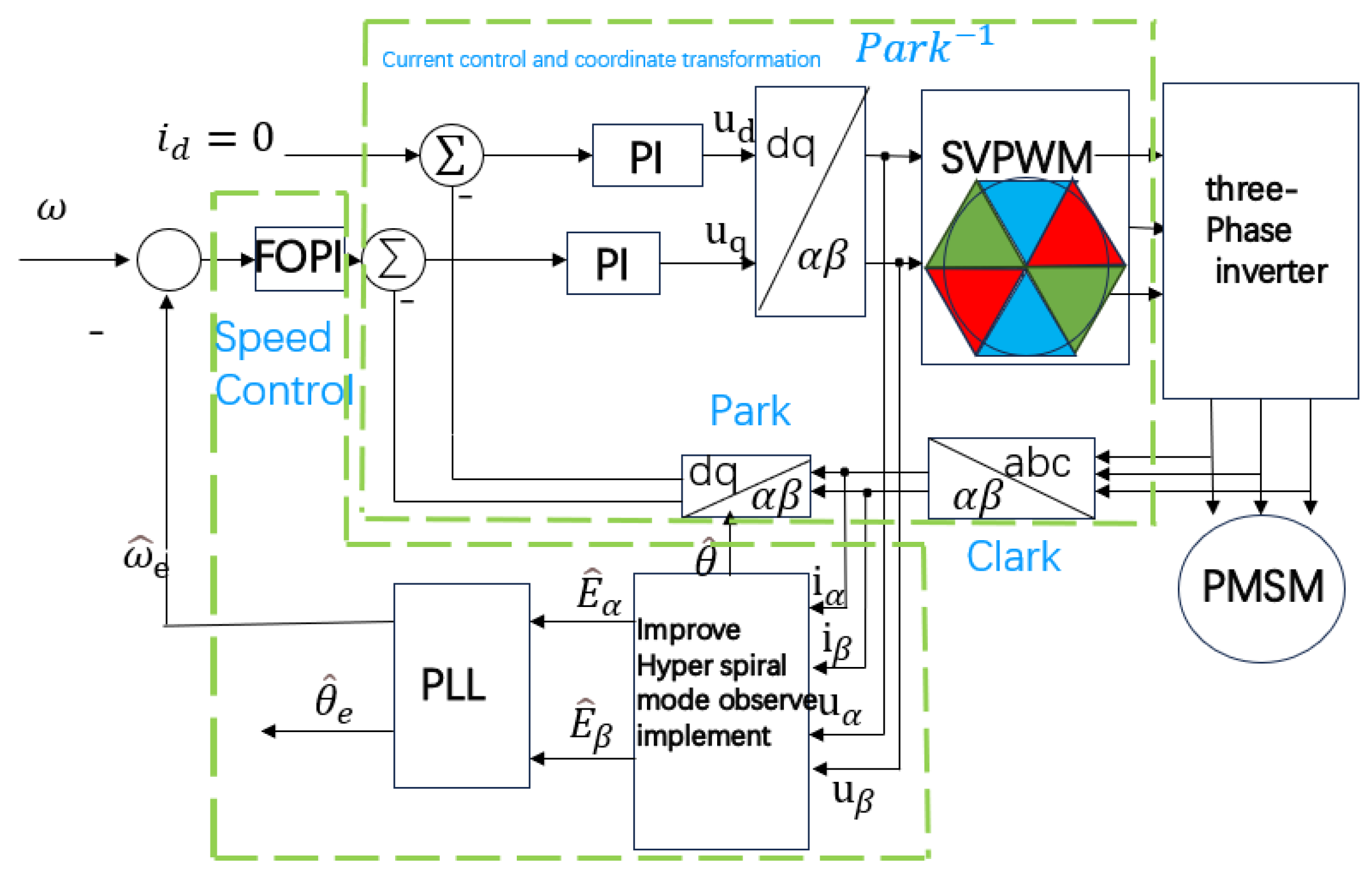
2. Mathematical Model of Permanent Magnet Synchronous Motor
3. Design of Improved Fuzzy Sliding Mode Observer
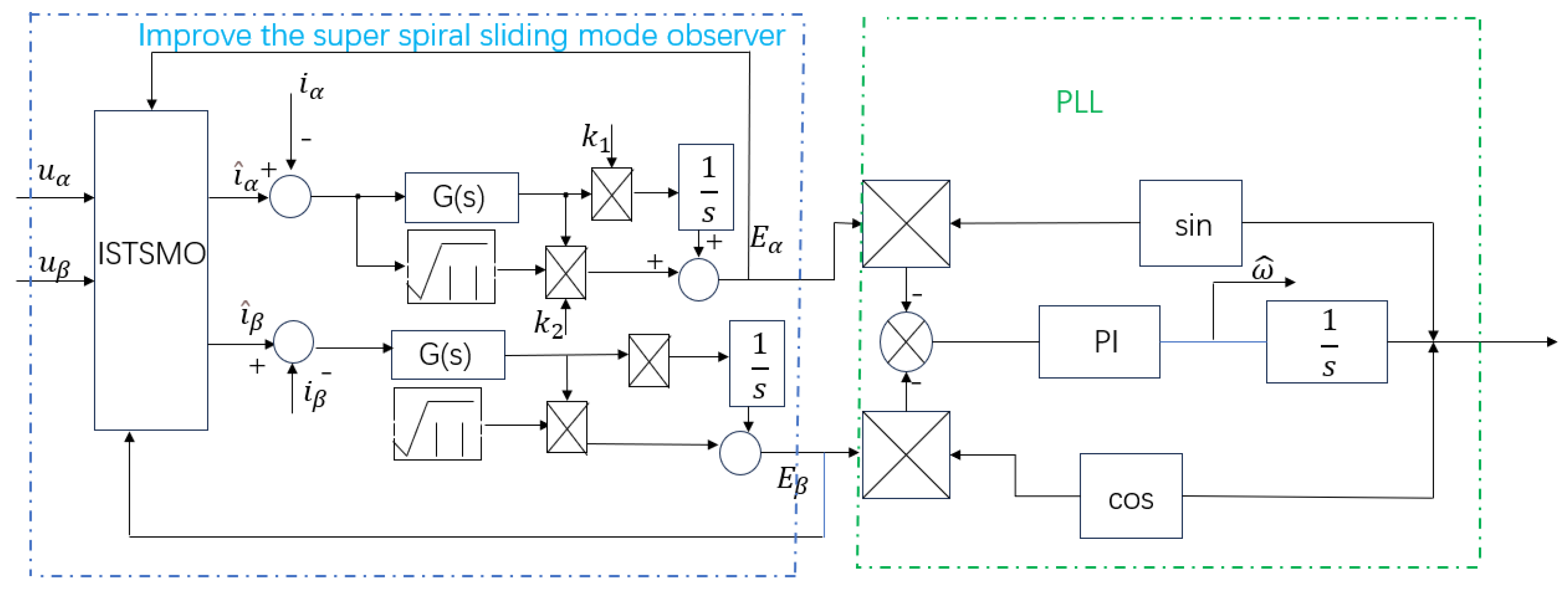
3.1. Mathematical Model of New Sliding Mode Observer
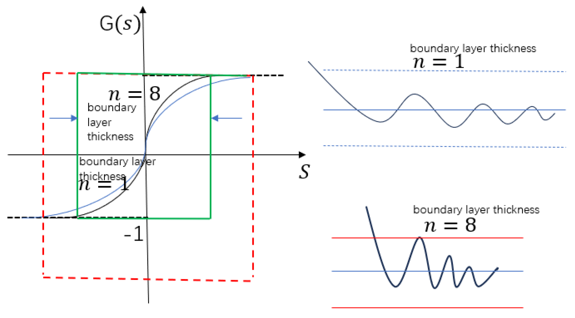
3.2. Design of Novel Sliding Mode Observer Based on Sin (Arctan(nx)) Function
3.3. Stability Analysis
- (1)
- The boundedness of functions: (that is because ).
- (2)
- The monotonicity of functions: take the derivative of :
- (3)
- Can be approximated:
3.4. Design of Fuzzy Controller
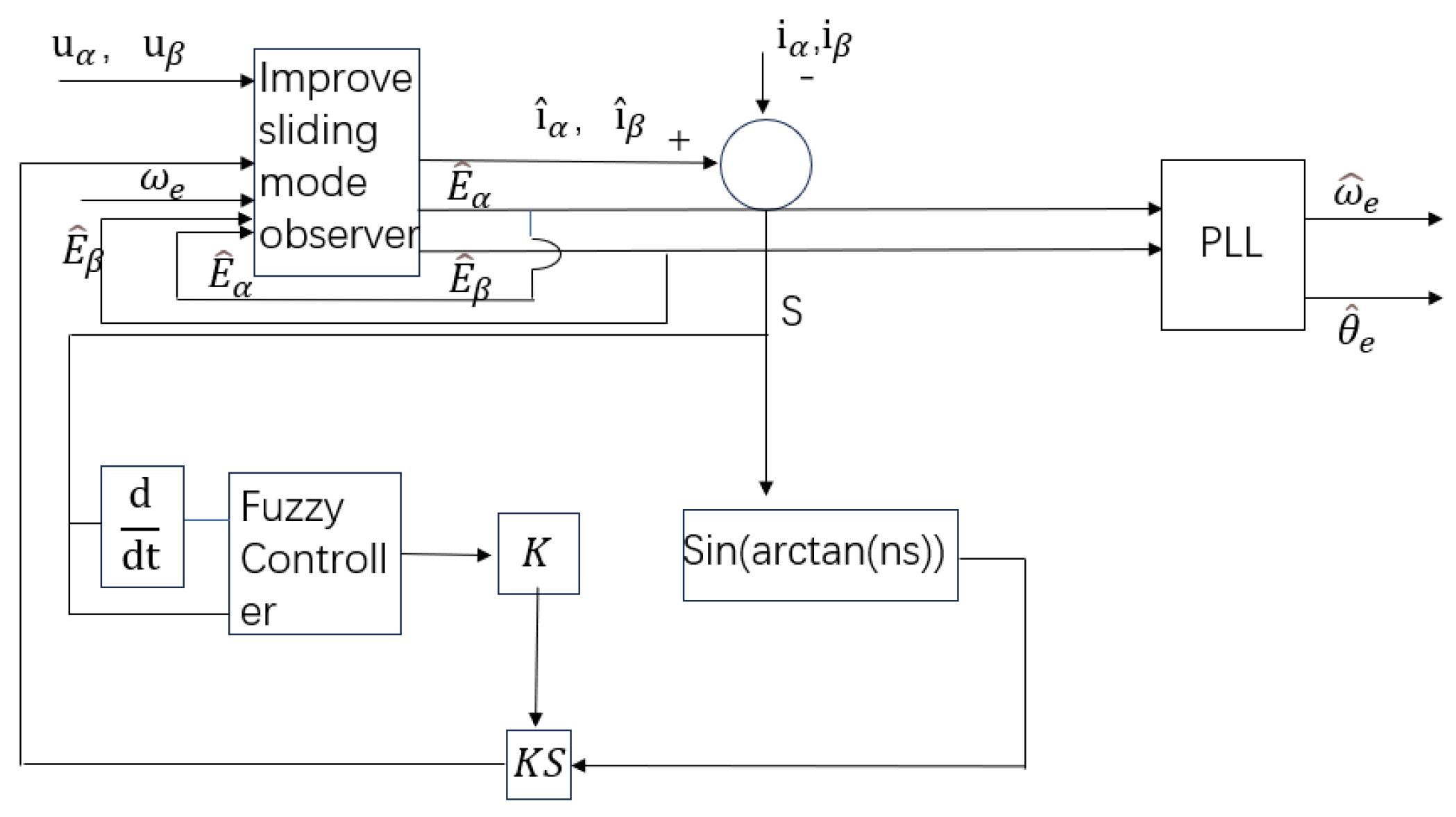
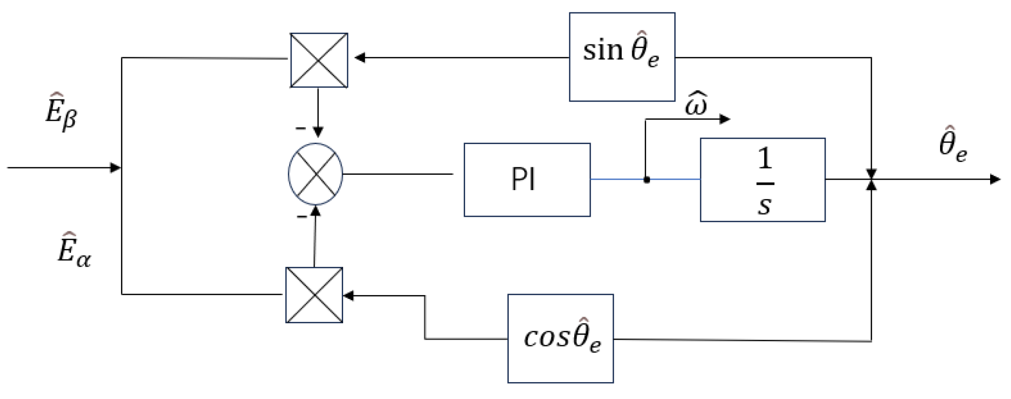
3.5. Fuzzy Improved Hyper Spiral Sliding Mode Observer
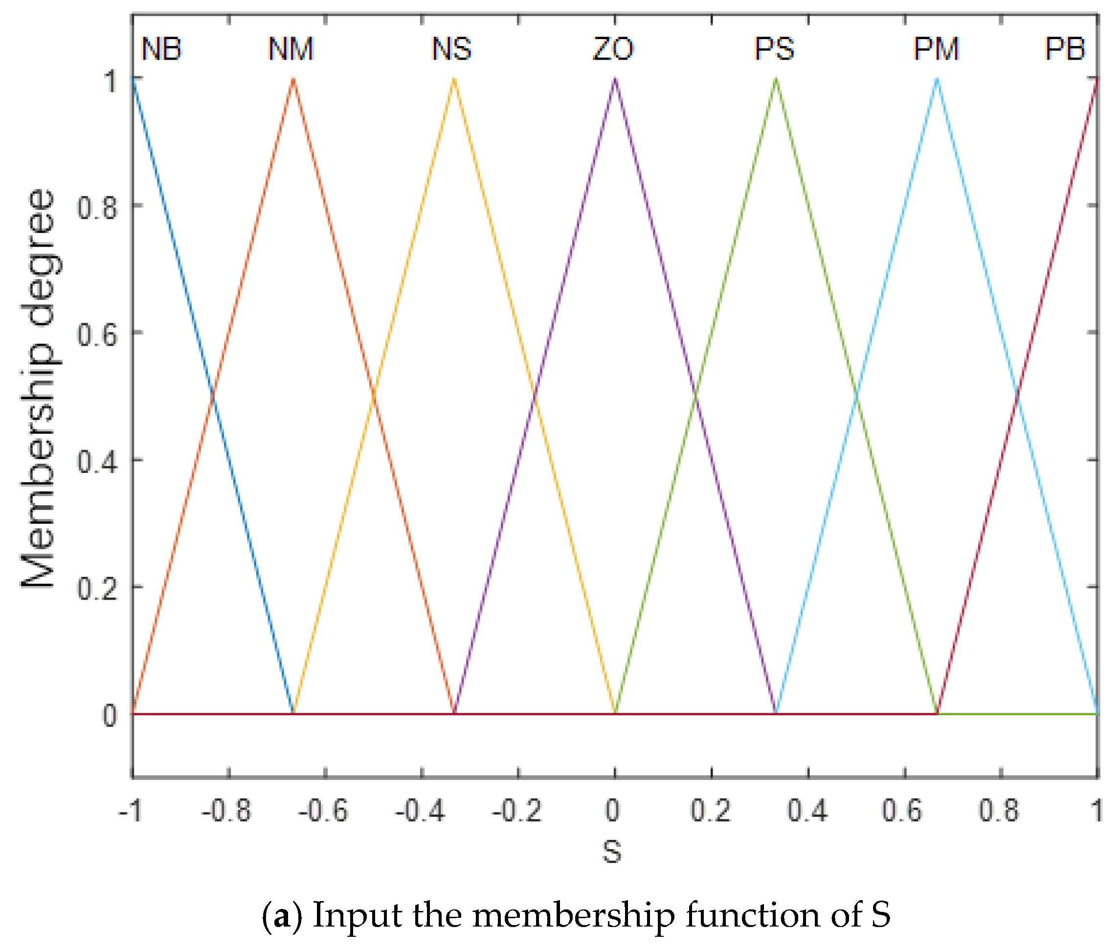
3.6. Sliding Mode Gain Fuzzy Design
4. Design of Fractional Order PID Controller
4.1. Fractional Calculus Theory
4.2. Controller Design
4.3. Parameter Tuning
- (1)
- Initialize PID parameters. First, use traditional methods to tune , , as a fundamental value.
- (2)
- Introduce fractional order , . For integral order , if the system requires a softer integration effect (such as eliminating overshoot), let . To quickly eliminate static errors, take (close to traditional integration). Differential order , if the system is sensitive to high-frequency noise, let to smooth the differential action. If damping is required to suppress oscillation, take .
- (3)
- Fine tune the gain parameters. After fixing and , readjust . Increasing accelerates the response, but may cause overshoot. Increasing reduces stability error, but may decrease stability. Increase , suppress oscillations, and amplify noise effects.
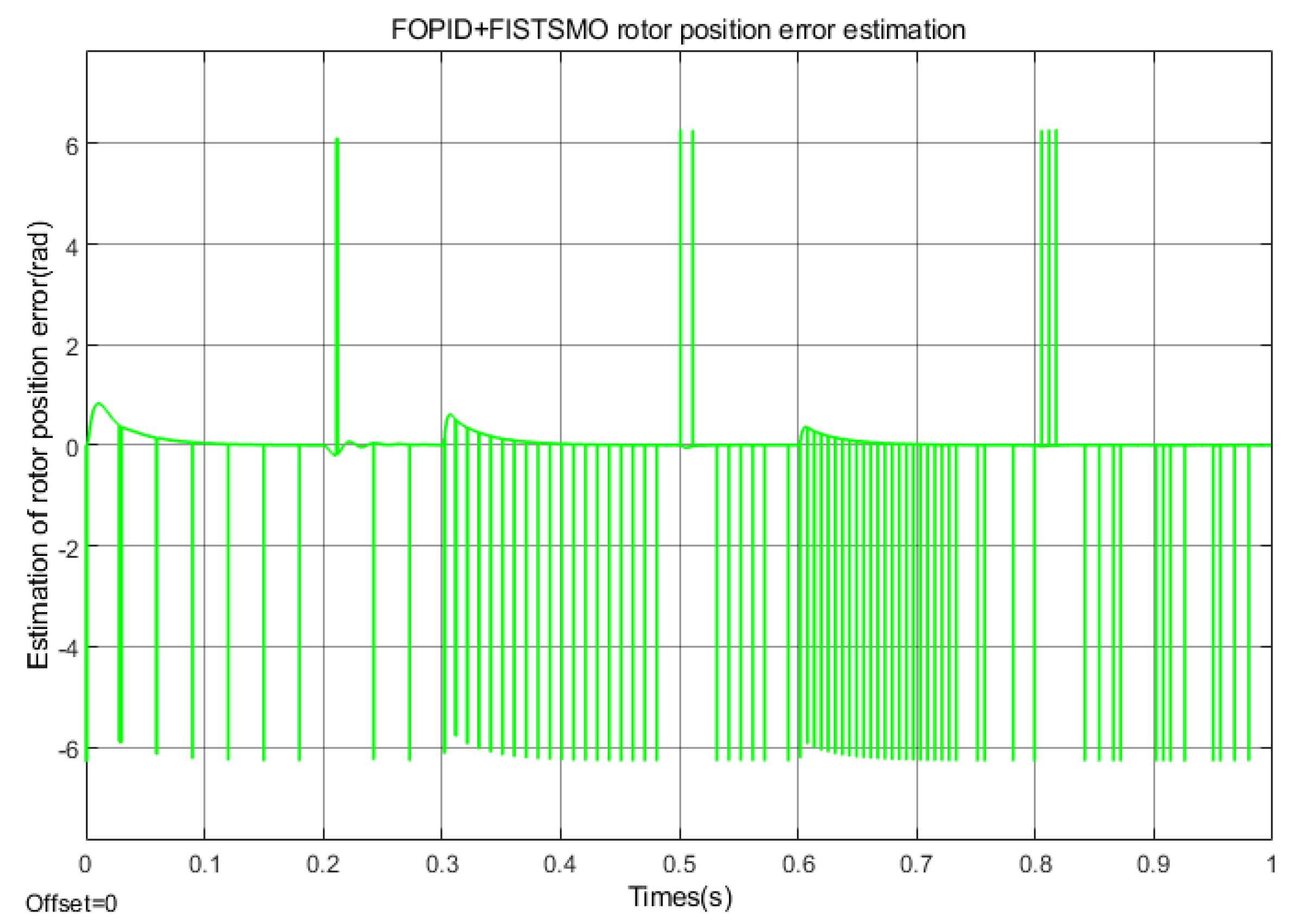
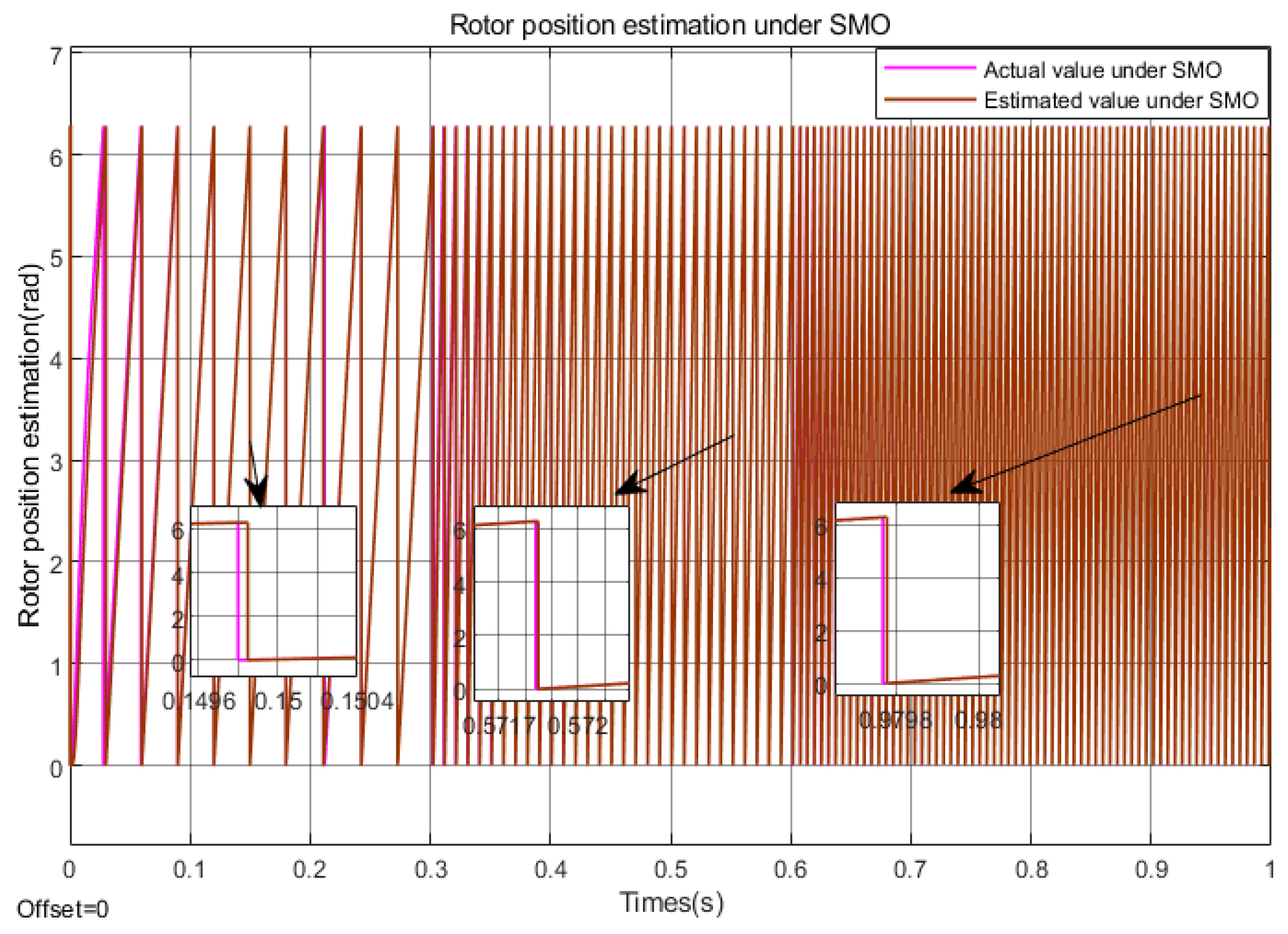
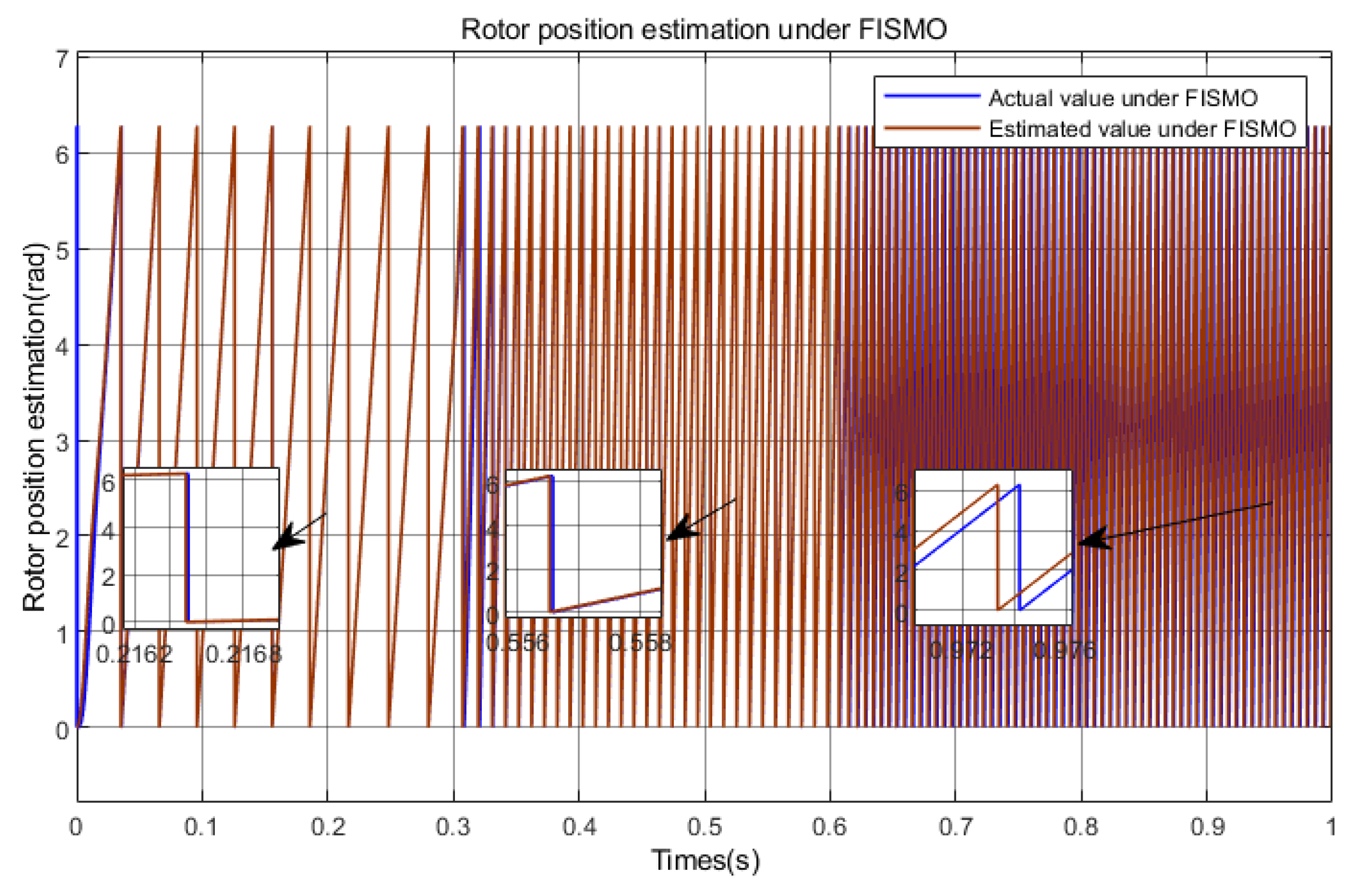
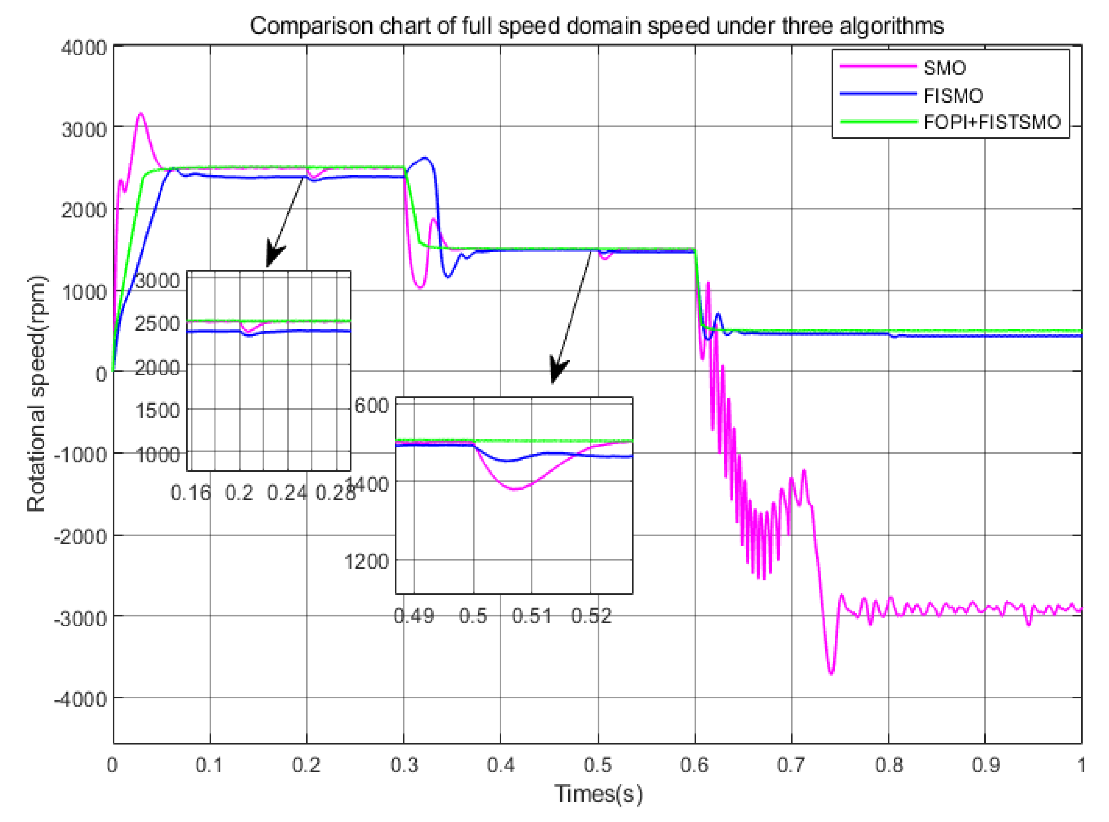
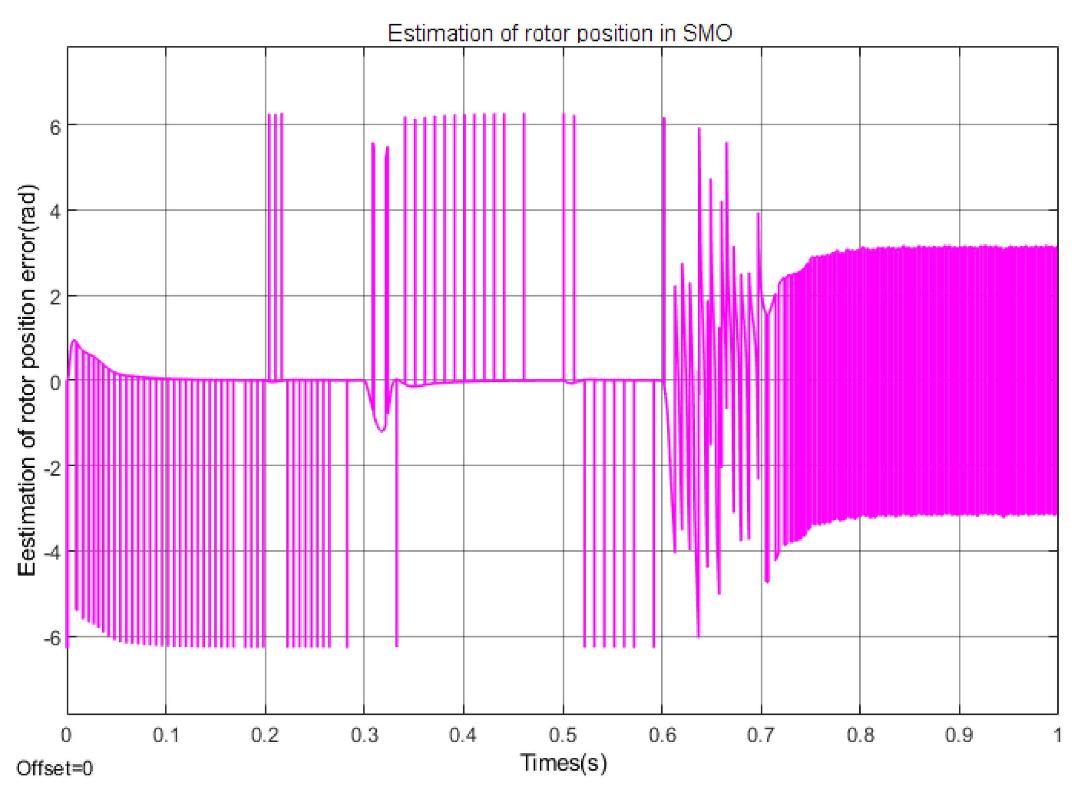
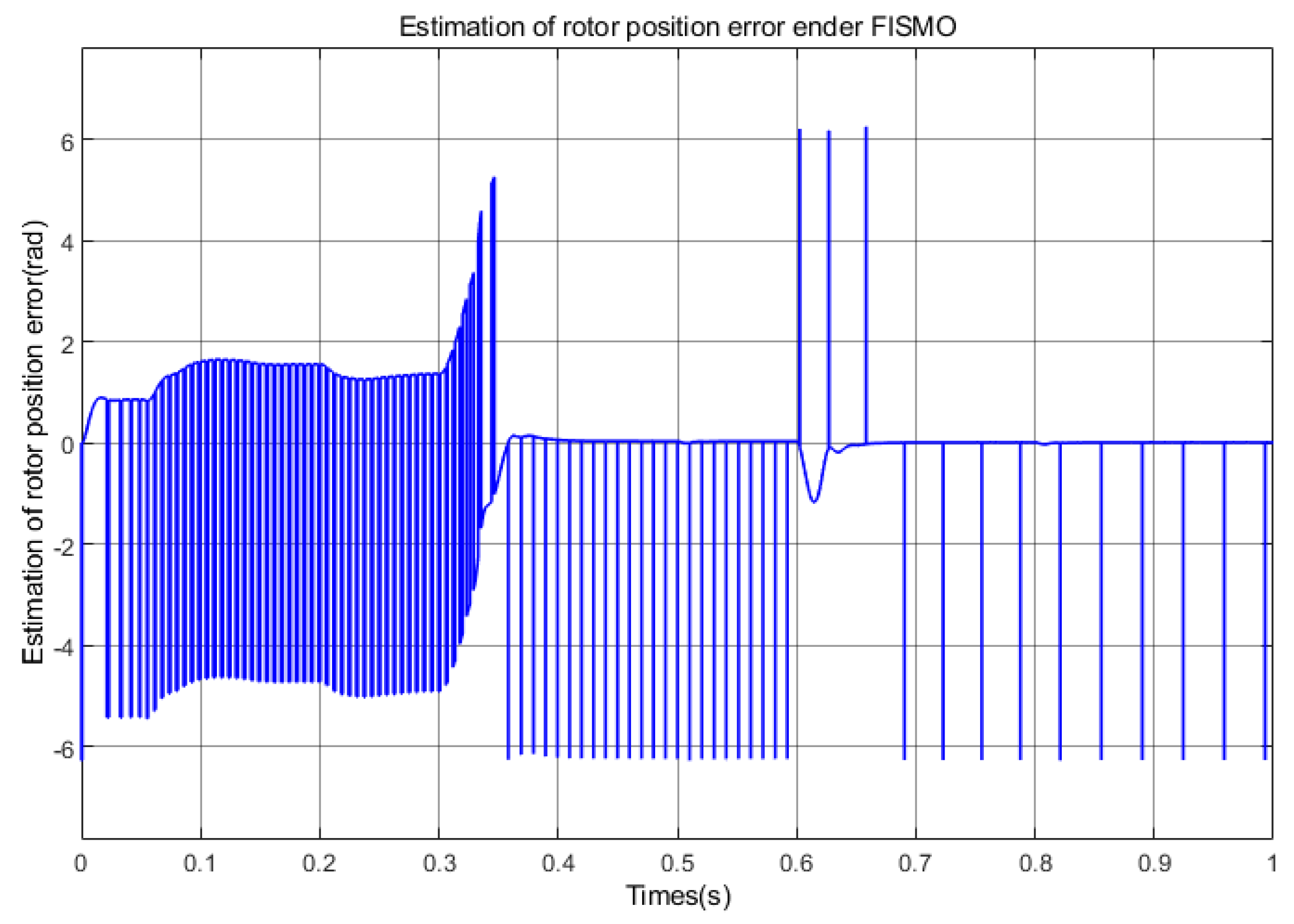
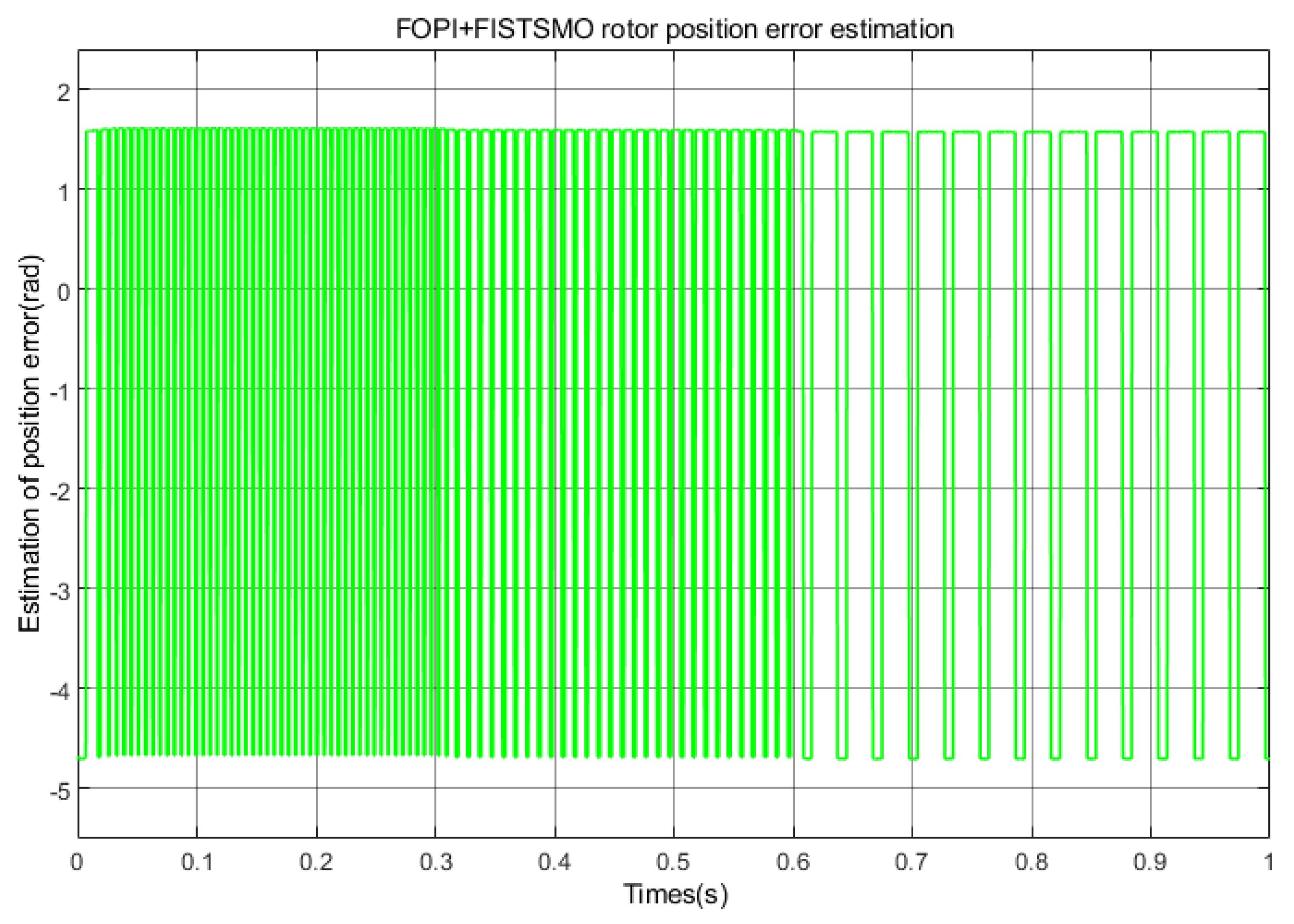
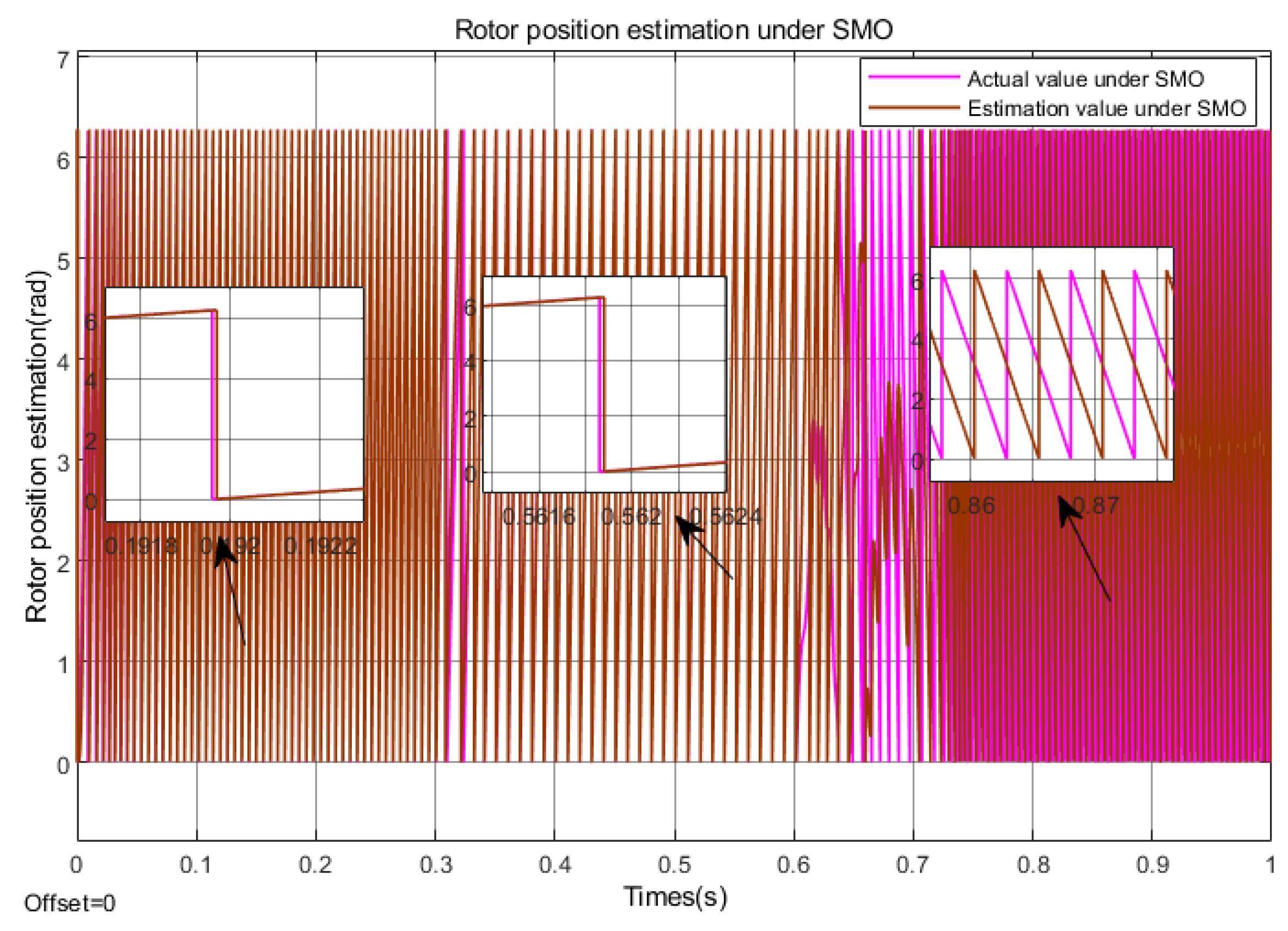
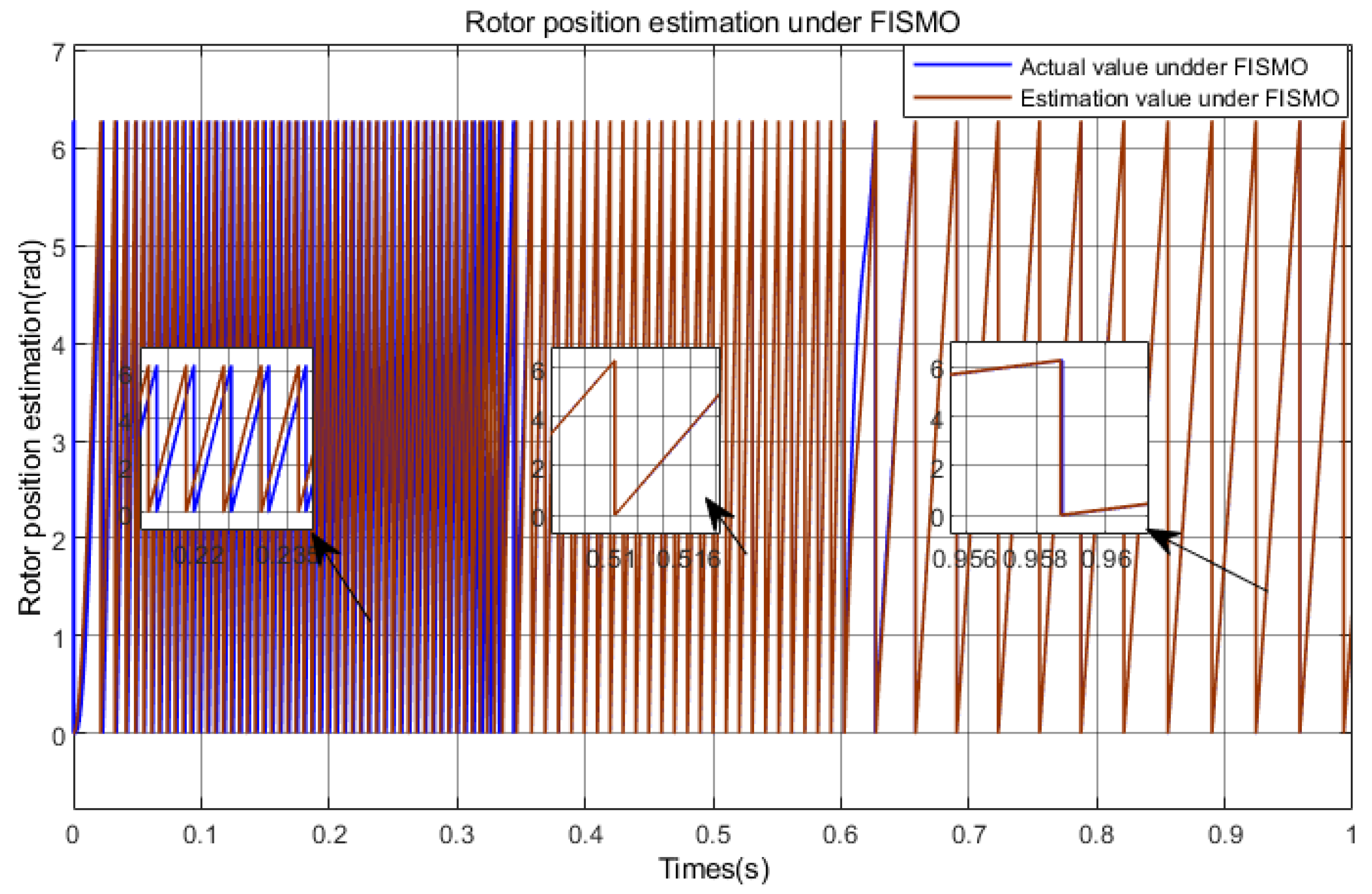
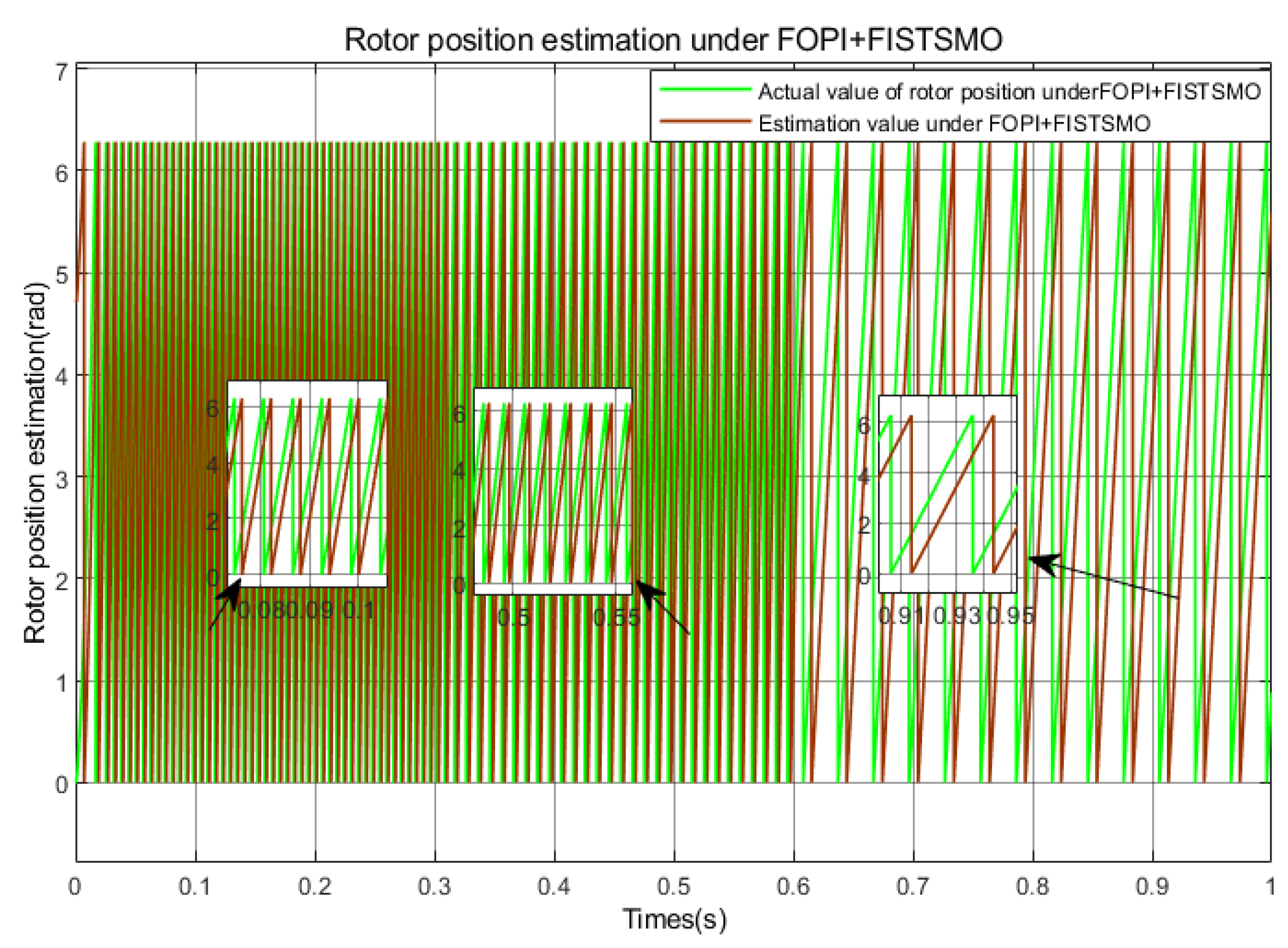
5. Simulation and Result Analysis
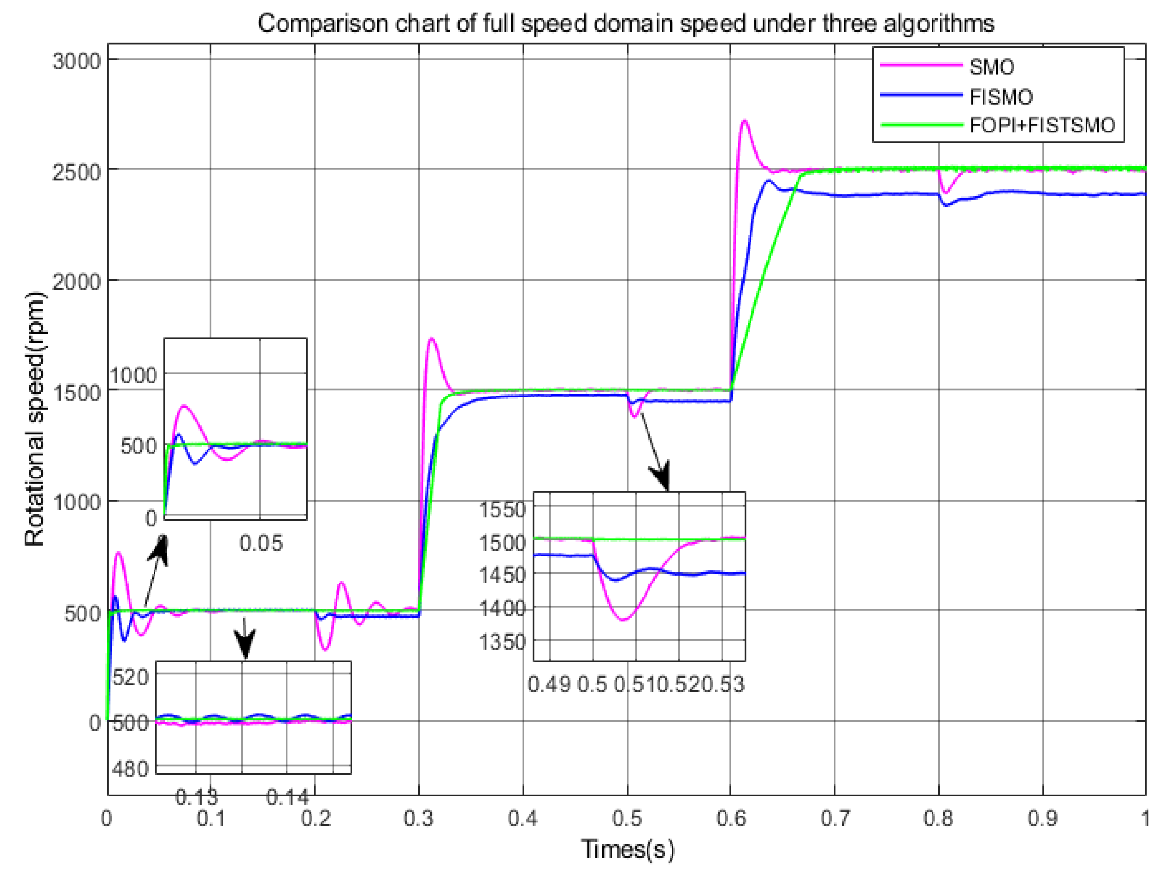
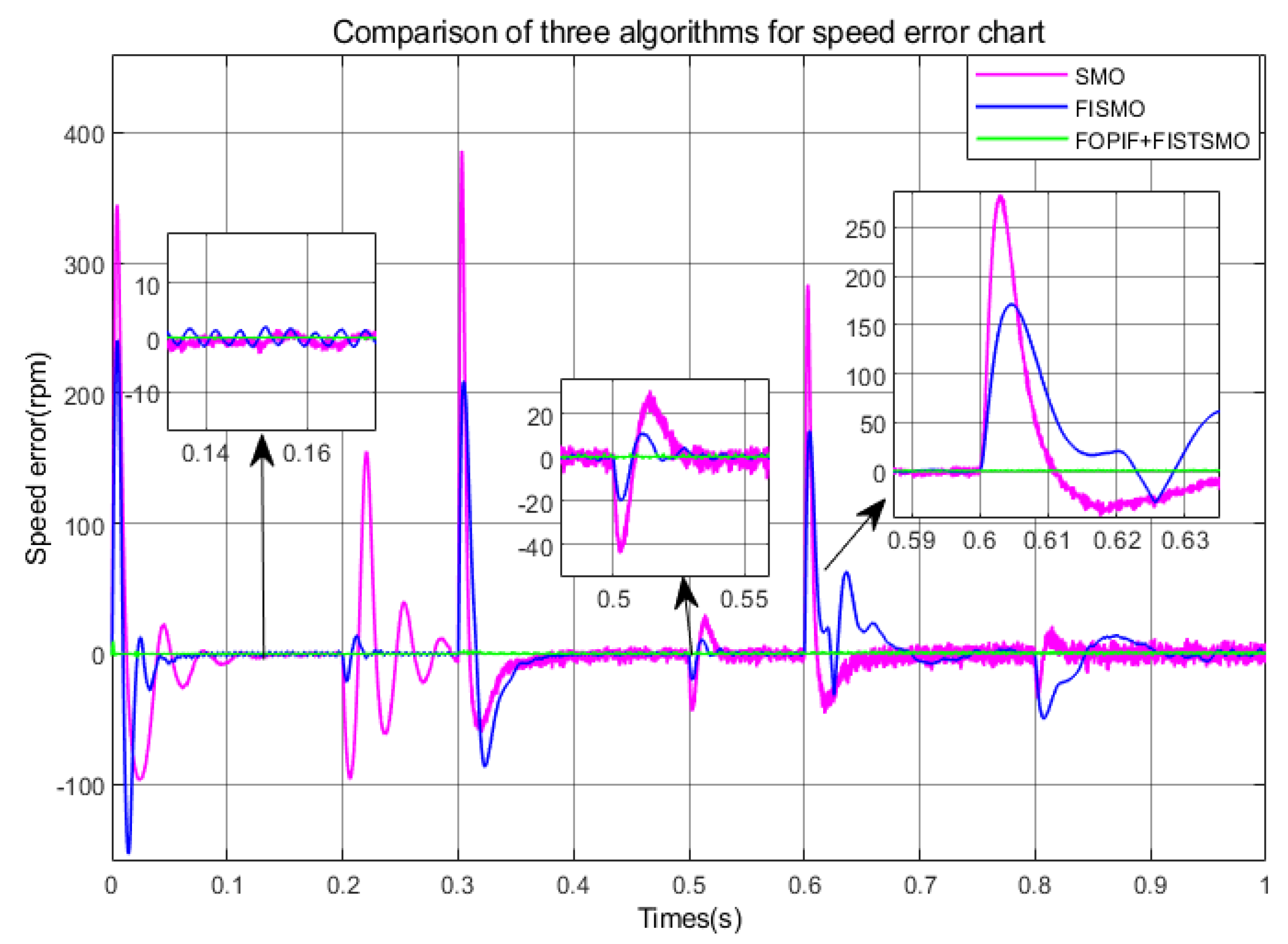
5.1. Sudden Load Changes During Acceleration
5.2. Sudden Load Change During Deceleration State
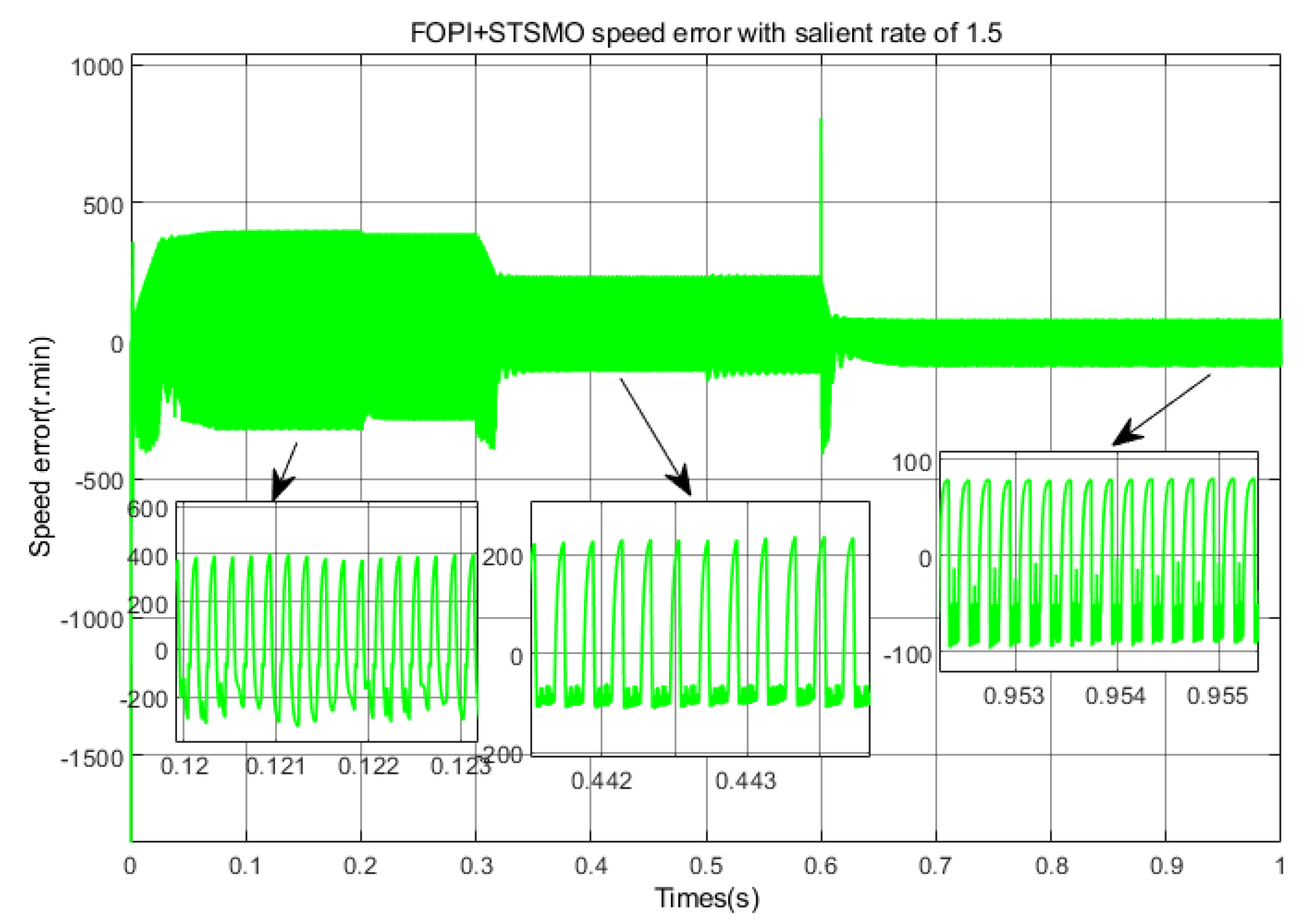
5.3. Applicability and Universality Analysis
6. Conclusions
Author Contributions
Funding
Data Availability Statement
Conflicts of Interest
References
- Boussak, M. Implementation and experimental investigation of sensorless speed control with initial rotor position estimation for interior permanent magnet synchronous motor drive. IEEE Trans. Power Electron. 2005, 20, 1413–1422. [Google Scholar] [CrossRef]
- Anh, H.P.H.; Khanh, P.Q.; Van Kien, C. Advanced PMSM Machine Parameter Identification Using Modified Jaya Algorithm. In Proceedings of the 2019 International Conference on System Science and Engineering (ICSSE), Dong Hoi, Vietnam, 20–21 July 2019; pp. 445–450. [Google Scholar]
- Termizi, M.S.; Lazi, J.M.; Ibrahim, Z.; Talib, M.H.N.; Aziz, M.J.A.; Ayob, S.M. Sensorless PMSM drives using Extended Kalman Filter (EKF). In Proceedings of the 2017 IEEE Conference on Energy Conversion (CENCON), Kuala Lumpur, Malaysia, 30–31 October 2017; pp. 145–150. [Google Scholar]
- Dai, S.; Wang, J.; Sun, Z.; Chong, E. An Improved Gradient-Based Optimization Algorithm for Synchronous Optimal Modulation of High-Speed PMSM Drives. In Proceedings of the 2021 IEEE International Electric Machines & Drives Conference (IEMDC), Hartford, CT, USA, 17–20 May 2021; pp. 1–8. [Google Scholar]
- Carter, S.R.; Praveen, P.; Varadhan, N.V.; Kowshik, S.; Gopinath, G. Field-Oriented Control (FOC) for Permanent Magnet Synchronous Motors (PMSM) in Electric Vehicle. In Proceedings of the 2023 International Conference on Next Generation Electronics (NEleX), Vellore, India, 14–16 December 2023; pp. 1–5. [Google Scholar]
- Cui, M.; Zhang, C.; Zhu, J. Realization of PMSM adjustable speed system based on sliding mode control. In Proceedings of the 2012 24th Chinese Control and Decision Conference (CCDC), Taiyuan, China, 23–25 May 2012; pp. 435–438. [Google Scholar]
- Teymoori, V.; Ghalebani, P.; Kamper, M.J.; Wang, R.-J. Sensorless Adaptive PI Control of High-Power Propulsion PMSM Based on Sliding-mode Extremum Seeking Algorithm. In Proceedings of the 2023 26th International Conference on Electrical Machines and Systems (ICEMS), Zhuhai, China, 5–8 November 2023; pp. 5158–5163. [Google Scholar]
- Liu, J. Fuchun Research and Progress on Sliding Mode Variable Structure Control Theory and Its Algorithms. Control. Theory Appl. 2007, 3, 407–418. [Google Scholar]
- Zhao, Y.; Liu, X. Speed Control for PMSM Based on Sliding Mode Control with a Nonlinear Disturbance Observer. In Proceedings of the 2019 Chinese Automation Congress (CAC), Hangzhou, China, 22–24 November 2019; pp. 634–639. [Google Scholar]
- Nicola, M.; Nicola, C.-I. Sensorless Control of PMSM using SMC and Sensor Fault Detection Observer. In Proceedings of the 2021 18th International Multi-Conference on Systems, Signals & Devices (SSD), Monastir, Tunisia, 22–25 March 2021; pp. 518–525. [Google Scholar]
- Bo, Y.; Lu, Q.; Xue, Y.; Zhou, X.; Zhang, G. Research on Adaptive PMSM Control Based on Novel Exponential Reaching Law. In Proceedings of the 2023 10th International Forum on Electrical Engineering and Automation (IFEEA), Nanjing, China, 3–5 November 2023; pp. 932–936. [Google Scholar]
- Xing, X.; Sheng, H. PMSM Sliding Mode Control Based on A New Exponential Reaching Law. In Proceedings of the 2021 3rd International Academic Exchange Conference on Science and Technology Innovation (IAECST), Guangzhou, China, 10–12 December 2021; pp. 199–203. [Google Scholar]
- Li, J.; Gao, Y.; Wang, L.; Yuan, H. A Sensorless Control System of PMSM Based on LADRC and SMO. In Proceedings of the 2020 International Conference on Artificial Intelligence and Electromechanical Automation (AIEA), Tianjin, China, 26–28 June 2020; pp. 66–71. [Google Scholar]
- Saadaoui, O.; Khlaief, A.; Abassi, M.; Chaari, A.; Boussak, M. Position sensorless vector control of PMSM drives based on SMO. In Proceedings of the 2015 16th International Conference on Sciences and Techniques of Automatic Control and Computer Engineering (STA), Monastir, Tunisia, 21–23 December 2015; pp. 545–550. [Google Scholar]
- Shi, J.; Liu, J.; Xu, J. Hybrid Position Sensorless Control Based on Estimation Position Error Switching for PMSM in Full Speed Range. In Proceedings of the IECON 2023—49th Annual Conference of the IEEE Industrial Electronics Society, Singapore, 16–19 October 2023; pp. 1–6. [Google Scholar]
- Chu, D. Research on Sensorless Vector Control of Permanent Magnet Synchronous Motor Based on Sliding Mode Observer; Harbin Institute of Technology: Harbin, China, 2015. [Google Scholar]
- Xinyu, S.; Xin, J. Research on position sensorless control of PMSM based on new SMO. In Proceedings of the 2024 39th Youth Academic Annual Conference of Chinese Association of Automation (YAC), Dalian, China, 7–9 June 2024; pp. 1508–1513. [Google Scholar]
- Amina Hasna, T.A.; Vijayasree, G. Sensorless Speed Control of PMSM Based on SMO with Traditional PLL and Tangent Function PLL. In Proceedings of the 2024 IEEE International Conference on Smart Power Control and Renewable Energy (ICSPCRE), Rourkela, India, 19–21 July 2024; pp. 1–5. [Google Scholar]
- Wu, B.; Yuan, Y. Research on PMSM Vector Control Based on Nonsingular Terminal Sliding Mode Observer. In Proceedings of the 2019 IEEE 3rd Advanced Information Management, Communicates, Electronic and Automation Control Conference (IMCEC), Chongqing, China, 11–13 October 2019; pp. 1773–1777. [Google Scholar]
- Yan, L.; Mao, Y. Position sensorless control of synchronous reluctance motor based on super spiral sliding mode observer. Softw. Guide 2024, 23, 105–113. [Google Scholar]
- Saadaoui, O.; Khlaief, A.; Abassi, M.; Chaari, A.; Boussak, M. Sensorless FOC of PMSM drives based on full order SMO. In Proceedings of the 2016 17th International Conference on Sciences and Techniques of Automatic Control and Computer Engineering (STA), Sousse, Tunisia, 19–21 December 2016; pp. 663–668. [Google Scholar]
- Zhang, X.; Jiang, Q. Research on Sensorless Control of PMSM Based on Fuzzy Sliding Mode Observer. In Proceedings of the 2021 IEEE 16th Conference on Industrial Electronics and Applications (ICIEA), Chengdu, China, 1–4 August 2021; pp. 213–218. [Google Scholar]
- Moreno, J.A.; Osorio, M. A Lyapunov approach to second-order sliding mode controllers and observers. In Proceedings of the 2008 47th IEEE Conference on Decision and Control, Cancun, Mexico, 9–11 December 2008. [Google Scholar]


| Function | Continuity | Differentiability | Boundary Value | Slope Adjustment Parameter |
|---|---|---|---|---|
| Discontinuous | Not Differentiable | Not have | ||
| Continuous | Differentiable | |||
| Continuous | Differentiable | (0, 1) | ||
| Continuous | Differentiable |
| NB | NM | NS | ZO | PS | PM | PB | |
| NB | PB | PB | PB | PB | PM | PM | PM |
| NM | PB | PB | PB | PM | PM | PM | PS |
| NS | PB | PM | PM | PS | ZO | ZO | PS |
| ZO | PM | PS | PS | ZO | PS | PS | PM |
| PS | PS | ZO | ZO | PS | PM | PM | PB |
| PM | PS | PM | PM | PM | PB | PB | PB |
| PB | PM | PM | PM | PB | PB | PB | PB |
| Parameter | Physical Meaning | Recommended Scope | Commissioning Method |
|---|---|---|---|
| Critical speed of gain segmentation | 10–30% rated speed | Experimental calibration | |
| Initial sliding mode gain | 20–100 | Adaptive adjustment through fuzzy rules | |
| Number of rules | The complexity of fuzzy controllers | items | Verify the necessity of each item one by one |
| Parameter | Numerical Value |
|---|---|
| Rated voltage/V | 311 |
| Rated speed/rpm | 3000 |
| Number of motor poles | 4 |
| Direct axis inductance/mH | 0.00097 |
| Cross axis inductance/mH | 0.00097 |
| ) | 0.0016 |
| 0.11 |
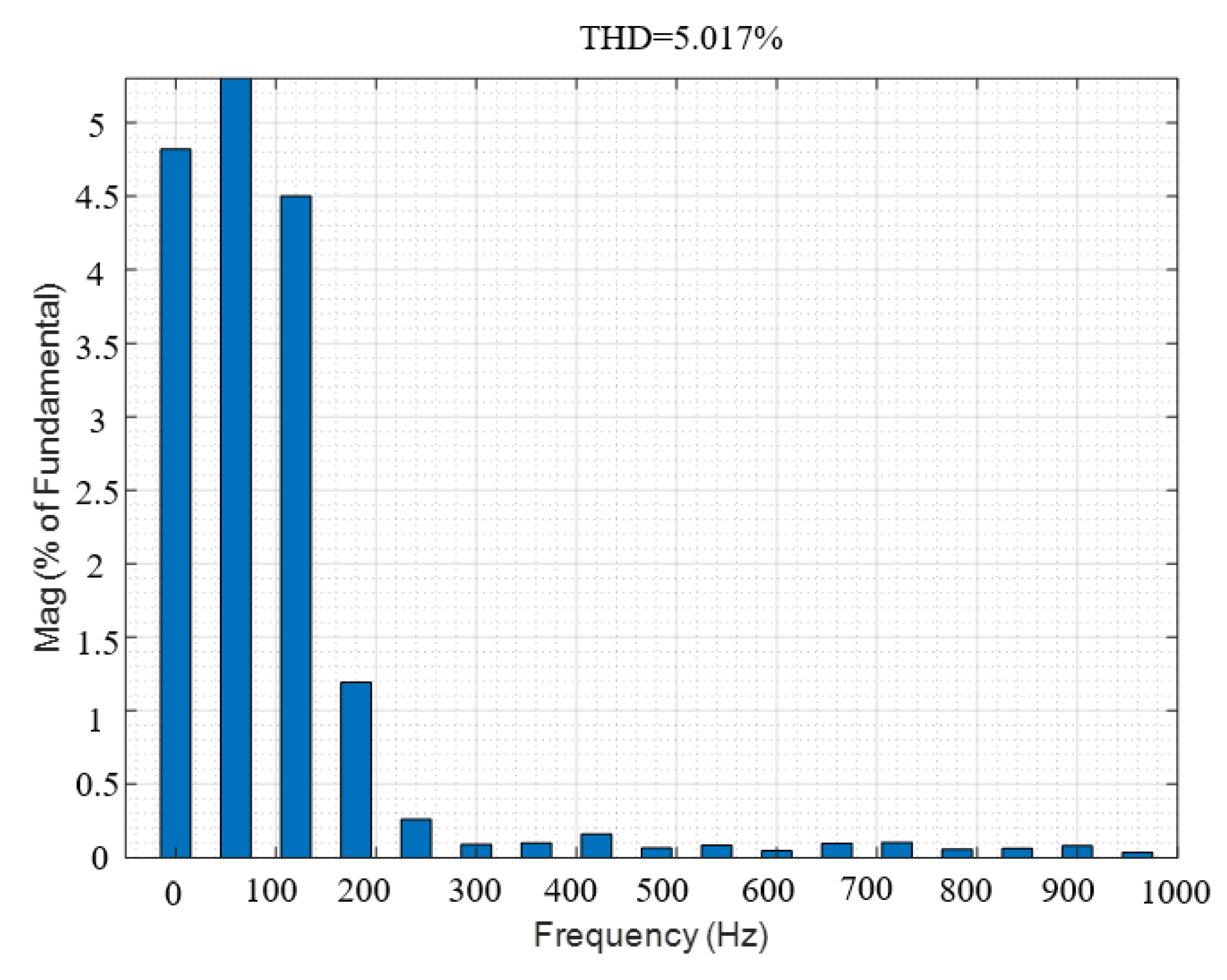
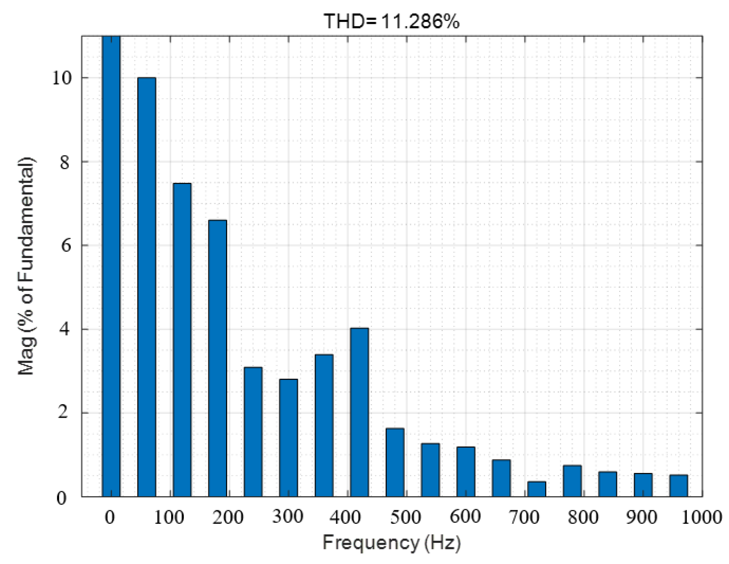
| Current THD (%) | Average Speed Error (%) | Average Overshoot (%) | |
|---|---|---|---|
| 1 | 5.017 | 1 | 1 |
| 1.2 | 7.04% | 5.2 | 5.24 |
| 1.5 | 11.2886 | 12.25 | 12.46 |
| Control Algorithm | Suppressing Vibration Effect | Control Accuracy | Dynamic Response Speed | Overshoot Ratio | Applicable Speed Range | Performance of Rotor Position Estimation |
|---|---|---|---|---|---|---|
| SMO | Poor | Medium | ) | ) | Medium speed | General (dependent on fixed gain) |
| FISMO | Better | Higher | ) | ) | Medium low speed | Good (Fuzzy Logic Optimization) |
| FOPI + FISTSMO | Best | Highest | ) | ) | All speed Range | Excellent (Fractional Order PI Adaptive) |
Disclaimer/Publisher’s Note: The statements, opinions and data contained in all publications are solely those of the individual author(s) and contributor(s) and not of MDPI and/or the editor(s). MDPI and/or the editor(s) disclaim responsibility for any injury to people or property resulting from any ideas, methods, instructions or products referred to in the content. |
© 2025 by the authors. Licensee MDPI, Basel, Switzerland. This article is an open access article distributed under the terms and conditions of the Creative Commons Attribution (CC BY) license (https://creativecommons.org/licenses/by/4.0/).
Share and Cite
Jiang, H.; Lv, X.; Fan, X.; Zhang, G. Research on Sensorless Control System of Permanent Magnet Synchronous Motor Based on Improved Fuzzy Super Twisted Sliding Mode Observer. Electronics 2025, 14, 1900. https://doi.org/10.3390/electronics14091900
Jiang H, Lv X, Fan X, Zhang G. Research on Sensorless Control System of Permanent Magnet Synchronous Motor Based on Improved Fuzzy Super Twisted Sliding Mode Observer. Electronics. 2025; 14(9):1900. https://doi.org/10.3390/electronics14091900
Chicago/Turabian StyleJiang, Haoran, Xiaodong Lv, Xiaoqi Fan, and Guangming Zhang. 2025. "Research on Sensorless Control System of Permanent Magnet Synchronous Motor Based on Improved Fuzzy Super Twisted Sliding Mode Observer" Electronics 14, no. 9: 1900. https://doi.org/10.3390/electronics14091900
APA StyleJiang, H., Lv, X., Fan, X., & Zhang, G. (2025). Research on Sensorless Control System of Permanent Magnet Synchronous Motor Based on Improved Fuzzy Super Twisted Sliding Mode Observer. Electronics, 14(9), 1900. https://doi.org/10.3390/electronics14091900