Energy-Efficient Federated Learning-Driven Intelligent Traffic Monitoring: Bayesian Prediction and Incentive Mechanism Design

Abstract

With the growing integration of the Internet of Things (IoT), low-altitude intelligent networks, and vehicular networks, smart city traffic systems are gradually evolving into an air–ground integrated intelligent monitoring framework. However, traditional centralized model training faces challenges such as high network load due to massive data transmission, energy management difficulties for mobile devices like UAVs, and privacy risks associated with non-anonymized road operation data. Therefore, this paper proposes an air–ground collaborative federated learning framework that integrates Bayesian prediction and an incentive mechanism to achieve privacy protection and communication optimization through localized model training and differentiated incentive strategies. Simulation experiments demonstrate that, compared to the Equal Contribution Algorithm (ECA) and the Importance Contribution Algorithm (ICA), the proposed method improves model convergence speed while reducing incentive costs, providing theoretical support for the reliable operation of large-scale intelligent traffic monitoring systems.

1. Introduction

The Internet of Things (IoT) enables the real-time interconnection of device data [1,2,3]; a low-altitude intelligent network (LAIN) provides network support for aerial vehicles such as unmanned aerial vehicles (UAVs) [4,5]; and the Vehicle-to-Everything (V2X) constructs a vehicle–road collaborative communication system [6,7,8,9]. With the deep integration of these three technologies, urban traffic systems are rapidly transitioning toward an air–ground integrated intelligent monitoring paradigm [10,11]. The cooperative sensing network composed of UAVs and unmanned ground vehicles (UGVs), leveraging its three-dimensional spatial coverage and multimodal data acquisition capabilities, has become the core infrastructure for smart city traffic flow monitoring [12,13,14].

In urban traffic management scenarios, each road is deployed with UGVs and UAVs equipped with pre-trained deep learning models [15,16]. UGVs utilize onboard sensors to monitor microscopic parameters such as ground vehicle queue lengths and driving speeds in real time, while UAVs dynamically capture macroscopic traffic conditions such as road congestion and traffic accidents from an aerial perspective. Through air–ground collaboration, the two form a comprehensive and multi-layered monitoring network [17,18,19].

The core objective of intelligent traffic monitoring is to enhance urban traffic efficiency, reduce accident rates, and provide timely, reliable data support for traffic scheduling and emergency response [20]. Achieving this requires the system to integrate multidimensional data sensing with real-time situational analysis. In practice, this involves utilizing UAVs for wide-area aerial coverage to quickly capture global traffic flow patterns; deploying UGVs for close-range, high-resolution monitoring at key traffic nodes; and applying edge computing together with federated learning for collaborative data processing. These components collectively enable intelligent decision-making in areas such as traffic signal optimization, rapid accident response, and route recommendation [21].

However, in the monitoring process, if clients transmit massive amounts of collected data directly to a central server for model training, it will not only overload network spectrum resources but also pose privacy risks [22,23]. Road operation data may expose key information such as regional traffic characteristics and accident distribution patterns. Additionally, the continuous large-scale data transmission significantly increases the power consumption of mobile devices such as UAVs [24]. Under high-load tasks, the battery life of clients may be greatly affected; in severe cases, it may even lead to the interruption of monitoring tasks, threatening the long-term stability and continuous operation of the system.

To address these challenges, federated learning (FL), as an innovative distributed model training mechanism, can effectively protect privacy and improve communication efficiency [25,26]. In the FL framework, model training is conducted on local devices, and clients only need to upload model update parameters instead of raw data, thereby preventing the leakage of sensitive information [27,28]. This approach not only enhances user privacy protection but also significantly reduces data transmission bandwidth requirements, improving overall system communication efficiency, particularly in scenarios involving massive data and frequent updates. However, in real-world FL applications, UAV and UGV clients differ significantly in terms of data acquisition dimensions, energy consumption characteristics, and communication resources. If all devices are allowed to participate in training indiscriminately, it may lead to unstable model performance, energy inefficiency, and reduced learning effectiveness. In other words, the strategy for client selection directly affects the training quality, system energy consumption, and the overall efficiency of traffic monitoring tasks. Moreover, in practical applications, devices face energy consumption and storage costs and will not participate in FL unconditionally [29,30,31]. Typically, model owners must provide incentives to attract devices to participate in training. Since model owners cannot directly obtain each client’s cost consumption and data quality, designing a reasonable incentive mechanism becomes a major challenge [32].

To solve this problem, this paper proposes an air–ground cooperative FL framework that integrates Bayesian prediction and incentive mechanism design. Specifically, in client selection, we construct a Bayesian optimization-based client contribution prediction model. By modeling the variation of the client’s loss function using a Gaussian process, the framework prioritizes devices with highly complementary parameter updates for federated aggregation. In incentive mechanism design, we develop a differentiated incentive function that provides additional rewards for high-data-quality clients, forming a positive feedback loop between “contribution level and incentive value”. These two components are well-suited for urban traffic monitoring scenarios, where UAVs typically provide high-altitude, wide-area observations, while UGVs offer detailed ground-level insights. By selecting and incentivizing clients based on their marginal contribution to the model, the proposed approach effectively mitigates the impact of non-independent and identically distributed (non-iid) datasets on model training and enhances the participation of high-contributing clients. This not only ensures the efficient use of incentive resources but also maintains high model performance.

In simulation experiments based on PyTorch (version 1.7.0), we compare our proposed method with the Equal Contribution Algorithm (ECA) and the Importance Contribution Algorithm (ICA) to verify its advantages in improving model training efficiency. The experimental results demonstrate that, compared to the traditional algorithms, our approach not only accelerates model convergence but also effectively reduces incentive costs.

The main contributions of this paper are as follows:

1. Proposed an air–ground integrated federated learning framework for smart city traffic flow monitoring: This framework combines the collaborative sensing capabilities of UAVs and UGVs, leveraging FL to achieve efficient privacy protection and communication optimization, adapting to the complex traffic monitoring demands of smart cities.

2. Developed a Bayesian optimization-based client contribution prediction model for client selection: By modeling the variation of the client’s loss function using a Gaussian process, the framework prioritizes high-contribution devices for federated aggregation, improving training efficiency and system performance.

3. Designed a differentiated incentive mechanism: The mechanism provides additional rewards for high-data-quality clients, encouraging active participation in FL and ensuring the sustainability and optimized performance of the system.

2. Related Works

In federated learning, client selection plays a critical role in improving training performance. For example, Asad et al. [33] proposed a joint communication and computation resource management algorithm aimed at minimizing global training costs. This approach effectively optimizes resource utilization and reduces overall overhead, thereby enhancing the efficiency of federated learning systems. Qu et al. [34] introduced an online client selection strategy based on Contextual Combinatorial Multi-Armed Bandit (CC-MAB), which optimizes client selection under budget constraints. By leveraging contextual information, the strategy enables more accurate decision-making in dynamic environments, significantly improving training performance and reducing regret, thus demonstrating strong practical effectiveness. However, most existing client selection algorithms achieve good performance at the cost of increased computational complexity. Such additional overhead can substantially burden the system and increase response latency. In intelligent traffic monitoring scenarios, central servers are required to process high-frequency data streams while ensuring real-time responsiveness, making it unsuitable to deploy client selection algorithms that are computation-intensive and resource-demanding. Therefore, there is an urgent need for a more lightweight, efficient algorithm that still maintains strong selection performance.

Traditional federated learning approaches often overlook the integration of incentive mechanisms in client selection. As self-interested and rational agents, UAVs and UGVs are typically unwilling to participate in federated learning without sufficient incentives [35]. Chen et al. [36] derived a contract-based incentive mechanism using the Lagrange multiplier method. Meanwhile, Xie et al. [37] proposed a blockchain-based UAV-assisted mobile crowdsourcing reputation incentive framework (BCFR). The combination of contract theory and reputation mechanisms has also been widely adopted to design incentive mechanisms for UAV participation in federated learning [35,38]. However, in the existing studies, incentive mechanisms are often designed independently of client selection strategies, and newly introduced incentive schemes may also incur additional computational overhead.

To address these issues, we propose a loss-based client selection mechanism. This method leverages the loss values naturally computed during training as the criterion for client selection, thereby eliminating any additional computational or communication overhead. As a result, it achieves highly efficient client selection while significantly reducing system costs, making it especially well-suited for resource-constrained intelligent traffic monitoring systems. Furthermore, we integrate incentive allocation directly into the client selection process to balance effectiveness and complexity. This integration constitutes the core motivation of our work, helping to bridge gaps in the existing research and advance the field in a complementary manner.

3. System Model

A complete urban traffic monitoring scenario should include several steps, such as real-time data collection, data analysis, and anomaly reporting [39].

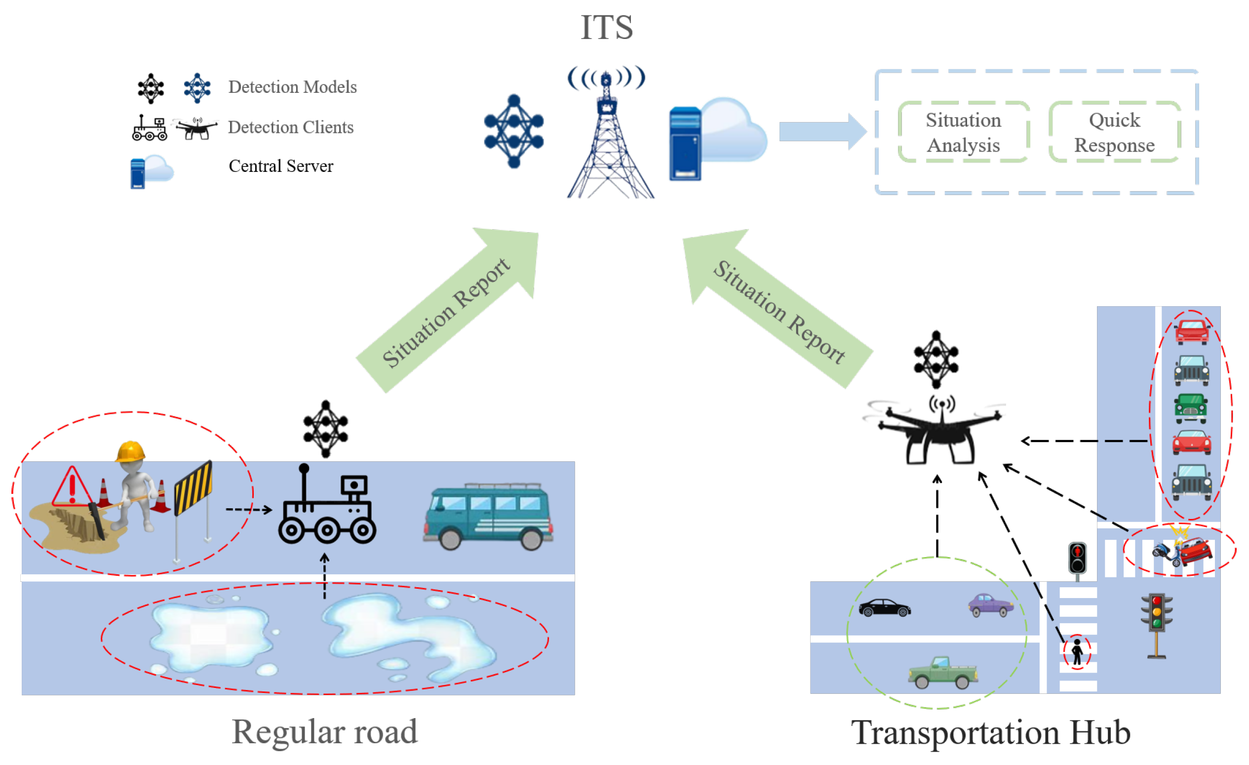
3.1. Scenario Description

In the urban traffic monitoring scenario, each city road is assigned a unique number and incorporated into the intelligent traffic management system. Each road is equipped with intelligent inspection devices, such as UAVs and UGVs, which are mounted with pre-trained deep learning models capable of real-time monitoring and analysis of traffic flow and accident situations [40].

UGVs mainly patrol on the ground, following pre-set routes and using onboard cameras and other sensors to capture real-time image data from the road. They detect key information such as vehicle queue lengths, average travel speeds, and congestion levels, as well as identify abnormal events, such as vehicle breakdowns, traffic accidents, or road closures. UAVs, on the other hand, conduct periodic patrols, providing a wider aerial view that covers key areas like main roads, highways, and intersections, enhancing the comprehensiveness of the monitoring.

Whenever a UGV or UAV detects an abnormal traffic situation, the system immediately triggers an anomaly reporting mechanism to transmit critical information to the traffic management center for quick response. The reported information includes road numbers, event types (e.g., traffic congestion, accidents, road closures), timestamps, and specific location details. In the traffic management center, the intelligent transportation system (ITS) analyzes the reported anomalies by combining historical traffic data and real-time monitoring information, generating the best response plan. For example, when the system identifies severe congestion on a certain road section, it can automatically adjust the green light duration of surrounding traffic lights to guide traffic flow. If a traffic accident is detected, the system will activate the emergency response mechanism, notifying traffic police, rescue vehicles, and the related departments, as we update the detour plan in real time within the navigation system to minimize the impact of the accident on overall traffic flow. A diagram of the scenario is shown in Figure 1.

Meanwhile, during the monitoring process, the clients continuously accumulate new image data. Since the traffic conditions of each road are different, the collected data are non-IID. As a result, the model struggles to maintain optimal performance across all roads [41]. To improve detection accuracy and adaptability, when the local data accumulated by the client reach a certain scale, the system will trigger local model training to incrementally update the original pre-trained model, enabling it to better adapt to the current road’s traffic patterns and unexpected situations [42].

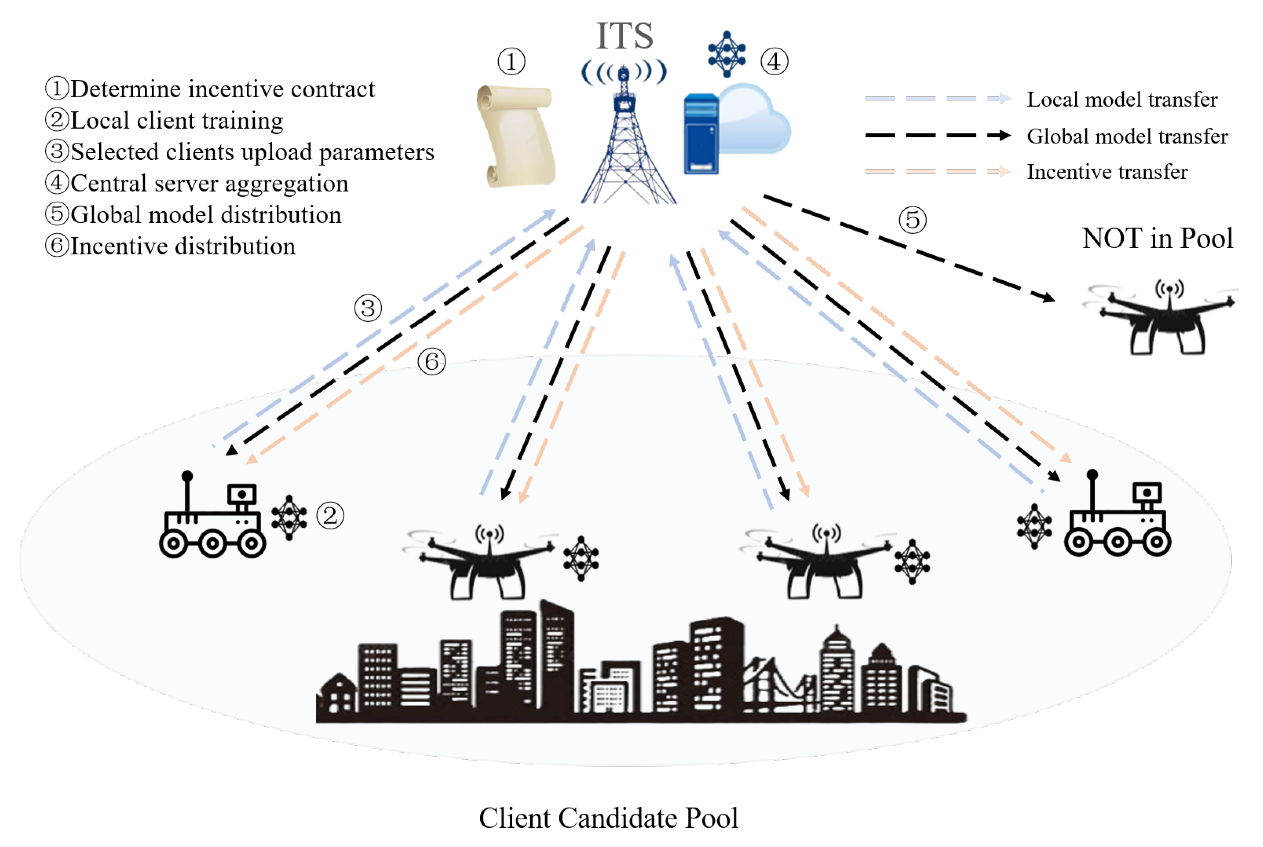
3.1.1. Federated Learning Model

Due to the differences in traffic conditions, traffic flow patterns, and types of emergencies across different roads, directly sharing raw monitoring data may lead to data privacy concerns and communication overhead issues. Therefore, the system adopts a federated learning architecture, where the UAVs and UGVs on each road perform model training locally and only upload the updated model parameters to the central server. This framework is vertically divided into the following two layers:

1. Traffic Monitoring Client Layer: UAVs and UGVs collect traffic flow, accident conditions, and other image data in their respective road areas and perform real-time analysis and anomaly detection using the current model. During the monitoring process, the devices continuously accumulate new local data and, when appropriate (such as when the data volume reaches a set threshold or when system resources permit), trigger local model training to optimize detection capabilities.

2. Central Server Layer: In each round of federated learning iterations, the central server collects local model updates from different road areas, performs federated aggregation to generate a more generalized global model, and provides incentives to the clients that have uploaded model updates. The aggregated model parameters are then distributed back to the clients to enhance the overall system’s traffic flow monitoring and anomaly detection capabilities.

To efficiently perform model parameter transmission, the system uses Orthogonal Frequency Division Multiple Access (OFDMA) technology for wireless communication [43], ensuring that clients from multiple roads can upload local model updates in parallel, reducing communication delays and bandwidth conflicts.

We assume the system consists of a central server and N local clients. In each model iteration, the system selects K clients from the N local clients to transmit their updates to the central server for parameter aggregation. The specific steps are as follows:

(1) In the global t-th round, the central server broadcasts the global model parameters ${\theta }_{\mathrm{t},\mathrm{global}}$, then selects K local clients.

(2) For each selected client $C_i$, where $i=1,2\dots \dots K$, $C_i$ receives the global model parameters ${\theta }_{\mathrm{t},\mathrm{global}}$ and performs local training using its local dataset $D_i$ and the Stochastic Gradient Descent (SGD) optimizer. The system sets the local training for $C_i$ to iterate for L rounds. During one round of local training, the output of the model is $\widehat{y_i}$, and the cross-entropy loss function is given by the following:

$$F_i\left({\theta }_t\right)=-{\displaystyle \frac{1}{D_i}}\sum _{i=1}^{D_i}[y_{i}log\left({\widehat{y}}_i\right)+(1-y_i)log(1-{\widehat{y}}_i)]$$

(1)

where $F_i\left({\theta }_{\mathrm{t}}\right)$ represents the loss function for client $C_i$, $D_i$ is the size of the dataset used by the client, $y_i$ is the true value of the i-th sample, and log represents the natural logarithm. Then, $C_i$ computes the local gradient $\nabla F_i\left({\theta }_{\mathrm{t}}\right)$ through backpropagation, and the model parameters ${\theta }_{\mathrm{t},\mathrm{local}}^{\mathrm{i}}$ are updated via SGD.

(3) After local training, the difference between the local and global model parameters is calculated. Specifically, for each parameter $\theta$ of $C_i$, we define $\Delta \theta$ to represent the difference, as follows:

$$\Delta {\theta }_t^i={\theta }_{\mathrm{t},\mathrm{local}}^i-{\theta }_{\mathrm{t},\mathrm{global}}$$

(2)

where ${\theta }_{\mathrm{t},\mathrm{local}}^i$ represents the local model parameters for client $C_i$ at round t, and ${\theta }_{\mathrm{t},\mathrm{global}}$ represents the global model parameters. This difference reflects the adjustments each client makes to the global model during local training.

(4) The selected K clients upload their $\Delta {\theta }_t^i$ to the central server via wireless channels. The central server aggregates the updates from each selected client to obtain the update $w_t=\lambda ·{\sum }_{\mathrm{i}=1}^k\Delta {\theta }_{\mathrm{t}}^{\mathrm{i}}$, where $\lambda$ is a hyperparameter. The global model parameters are then updated using the following formula:

$${\theta }_{\mathrm{t}+1,\mathrm{global}}={\theta }_{\mathrm{t},\mathrm{global}}+w_t$$

(3)

(5) The above-mentioned steps are repeated until the model reaches the convergence condition, $|F\left({\theta }_t\right)-F\left({\theta }_{t-1}\right)|\le \epsilon$, where $\epsilon$ is a preset positive threshold, and $F\left(\theta \right)$ represents the global cross-entropy function. Alternatively, the process can stop when other termination conditions are met.

The federated learning process with incentives is shown in Figure 2.

3.1.2. Communication Model

In our OFDMA scheme, we assume additive Gaussian white noise (AWGN) for channel noise, neglecting other interferences. While real-world channels are subject to larger impairments like fading and Doppler effects, modeling these requires complex simulations. Since this work focuses on client scheduling and incentive mechanisms, we adopt the AWGN assumption to isolate the key aspects. This simplification has been commonly used in prior FL studies (e.g., [44,45]) thus validating our approach.

The scheme has N orthogonal subchannels, where $N\ge K$, and each channel has bandwidth W. In the t-th round, the uplink delay of client $C_k$ to the central server, ${\tau }_k^{up}\left(t\right)$, is calculated by the following formula:

$${\tau }_k^{up}\left(t\right)={\displaystyle \frac{s_k^{up}\left(t\right)}{r_k^{up}\left(t\right)}}$$

(4)

where $s_k^{up}\left(t\right)$ is the amount of data to be uploaded, and $r_k^{up}\left(t\right)$ is the transmission rate of client $C_k$ to the central server, given by Shannon’s formula, as follows:

$$r_k^{up}\left(t\right)=W{log}_2\left(1+{\displaystyle \frac{p_k^{up}{h}_k}{{\sigma }^2}}\right)$$

(5)

where $p_k^{up}$ is the transmission power of client $C_k$, $h_k$ is the channel gain of client $C_k$, and ${\sigma }^2$ is the noise power.

Additionally, the transmission energy consumption of client $C_k$ is expressed by the following formula:

$$E_k^{com}\left(t\right)={\tau }_k^{up}\left(t\right)p_k^{up}$$

(6)

3.1.3. Computation Model

Training at client $C_k$ also incurs energy consumption, which is given by the following formula:

$$E_k^{Cal}=\kappa Cy{c}_k{D}_k{f}_k^2$$

(7)

where $Cy{c}_k$ (cycles/sample) is the number of CPU cycles required by client $C_k$ to process one data sample, $D_k$ (sample) is the length of the data sample that $C_k$ needs to process, $f_k$ (cycles/s) represents the CPU computation capacity (CPU frequency) of client $C_k$, and $\kappa$ is the effective capacitance parameter of the computing chipset.

Additionally, the time required for one local model training at the client is given by the following formula:

$${\tau }_k^{cal}={\displaystyle \frac{Cy{c}_k{D}_k}{f_k}}$$

(8)

3.2. Optimization Problem Description

In the t-th round of global iteration, the total energy consumed by client $C_k$ to participate in model training is denoted by $E_k\left(t\right)$, as expressed in the following equation:

$$E_k\left(t\right)=L{E}_k^{cal}\left(t\right)+E_k^{com}\left(t\right)$$

(9)

Meanwhile, in the t-th round of global iteration, the total time required by client $C_k$ to participate in model training is ${\tau }_k\left(t\right)$, which can be calculated as follows:

$${\tau }_k\left(t\right)=L{\tau }_k^{cal}\left(t\right)+{\tau }_k^{up}\left(t\right)$$

(10)

The energy consumption $E_k\left(t\right)$ and elapsed time ${\tau }_k\left(t\right)$ of a client’s participation in training are defined by Equations (9) and (10), respectively, and both of them directly determine whether they satisfy the resource constraints of the system (Equations (11a) and (11b)). Based on this, the optimization problem (P1) accelerates the model convergence by maximizing the cumulative client contributions and selecting the optimal set of clients under the energy and delay constraints. Therefore, we can formulate the optimization problem (P1) as follows:

$$\left(P1\right)\underset{{\mathcal{S}}^t}{max}\sum _{t=1}^T\sum _{k\in {\mathcal{S}}^t}{Y}_k\left(t\right)$$

(11)

$$\begin{array}{cc}\hfill \mathrm{subject}\mathrm{to}{E}_k\left(t\right)& \le E_{max},\forall k\in {\mathcal{S}}^t\hfill \end{array}$$

(11a)

$$\begin{array}{cc}\hfill {\tau }_k\left(t\right)& \le {\tau }_{max},\forall k\in {\mathcal{S}}^t\hfill \end{array}$$

(11b)

$$\begin{array}{cc}\hfill |{\mathcal{S}}^t|& =K\hfill \end{array}$$

(11c)

where $Y_k\left(t\right)$ is the contribution of client $C_k$ to the convergence of the global model in the t-th round; ${\mathcal{S}}^t$ is the set of clients selected in the t-th round; T is the total number of training rounds; $E_{max}$ is the energy consumption limit for each client; and ${\tau }_{max}$ is the maximum acceptable delay for the clients.

From the expression of (P1), it is clear that if we choose the K clients that contribute the most to the global model in each round, we can maximize the overall contribution ${\sum }_{k\in {\mathcal{S}}^t}{Y}_k\left(t\right)$ in each round and thus maximize the convergence speed of the global model. The complexity of this problem arises from the unpredictable number of global training rounds T, and the fact that each client’s contribution $Y_k\left(t\right)$ may change dynamically in each round. Therefore, we cannot calculate the contribution of each client in advance and directly select the K clients with the highest contributions before each training round.

Bayesian prediction is an inference method based on prior distribution and observational data to update the posterior distribution, making it particularly suitable for scenarios with high uncertainty [46]. Additionally, in the practical traffic flow monitoring scenario, each client faces energy consumption and storage costs, with significant differences in traffic flow patterns and accident frequencies across different roads, leading to unequal contributions from each client. Therefore, to encourage local model training and ensure that the federated learning framework adapts more effectively to the traffic characteristics of different roads, we can incentivize clients with higher contributions to enhance the overall model’s performance. This will be detailed in the next section.

4. Client Selection and Incentive Algorithm Design Based on Bayesian Prediction

We define $R_k\left(t\right)$ as the incentive provided by the central server to client $C_k$ at the t-th round. The incentive can be in the form of money, points, etc. The utility function $U_k\left(t\right)$ of client $C_k$ can be expressed as follows:

$$U_k\left(t\right)=R_k\left(t\right)-E_k\left(t\right)=R_k\left(t\right)-L{E}_k^{cal}-E_k^{com}$$

(12)

The central server must consider the reasonable demands of clients when designing contracts; each client will only participate in the federated learning task if its utility is not less than zero, i.e., $U_k\left(t\right)=R_k\left(t\right)-E_k\left(t\right)\ge 0$. Additionally, to reduce the delay in each round, no incentive will be given to clients whose total delay exceeds the maximum delay.

$$U_k\left(t\right)=\left\{\begin{array}{cc}{R}_k\left(t\right)-E_k\left(t\right),\hfill & {\tau }_k\left(t\right)\le T_{max}\hfill \\ -E_k\left(t\right),\hfill & {\tau }_k\left(t\right)>T_{max}\hfill \end{array}\right.$$

(13)

Thus, we have described the potential rewards each participating client can obtain in each round. Next, we need to design a reasonable reward function $R_k\left(t\right)$ to reflect the value of the client’s data in each training round. Ideally, the calculation of the function value should require minimal additional computation to reduce energy consumption. Therefore, we use the client’s loss function during model training for evaluation. Since the loss function must be computed during model training, choosing the loss function does not incur additional computation. To converge faster, we will select clients that cause the global model’s loss function to decrease more quickly.

We design a loss prediction method based on Bayesian prediction. First, a client is randomly selected for initialization, and then, each time, a client contributing more to convergence is selected. Each selection involves the following three steps:

1. Predicting the loss function value for the selected client: Assume that client $C_k$ is selected in the current round. We first need to predict the loss of client $C_k$. Since the client’s loss in each round has randomness, in Bayesian prediction, we assume the prior distribution of the client’s loss is Gaussian. Thus, the variation in the loss of all clients in the t-th round can be modeled as follows [45]:

$$\Delta I^t=[\Delta I_1^t,\dots ,\Delta I_N^t]\sim N\left({\mu }^t,{\Sigma }^t\right)$$

(14)

where ${\mu }^t$ is the mean vector of client loss changes; ${\Sigma }^t$ is the variance vector; and $\Delta I_1^t,\dots ,\Delta I_N^t$ represent the loss changes of clients $C_1,\dots ,C_N$. The predicted loss change for client $C_k$ is as follows:

$$\Delta \widehat{I_k^t}={\mu }_k^t-{\alpha }_k^t{\sigma }_k^t$$

(15)

where ${\alpha }_k^t$ is a tuning parameter that controls the trade-off between exploration and exploitation of uncertainty. If ${\alpha }_k^t$ is large, the algorithm prefers clients with high loss volatility (large ${\sigma }_k^t$). Such clients may have unstable current contributions but high exploration potential. If ${\alpha }_k^t$ is small, the algorithm prefers to trust clients with stable historical performance (${\mu }_k^t$ dominant) and prioritizes known high contributors. And ${\sigma }_k^t=\sqrt{{\sum }_{k,k}^t}$ is the standard deviation of the loss change for client $C_k$. Here, ${\sum }_{k,k}^t$ represents the diagonal elements of the matrix ${\sum }^t$, i.e., the variance of client $C_k$. The top hat on $\widehat{I_k^t}$ indicates that this is a posterior distribution-based loss change prediction.

2. Selecting the client by the model owner: Each time, a client is selected to minimize the posterior expected total loss. Substituting the loss change prediction formula for client $C_k$, we obtain the following formula:

$$k^{*}=argmin\sum _i{p}_i\Delta {\widehat{I}}_k^t=arg\underset{k}{min}\sum _i{p}_i{\mu }_i-{\alpha }_k^t\sum _i{p}_i{\sigma }_i{r}_{i,k}$$

(16)

where i represents the selected clients; and $p_i$ is the weight of client $C_i$. Pearson’s correlation coefficient $r_{i,k}={\displaystyle \frac{{\Sigma }_{i,k}}{{\sigma }_i{\sigma }_k}}$ is used to indicate the correlation between clients; the closer $r_{i,k}$ is to 0, the higher the independence between clients, and the more suitable they are for joint participation to cover diverse data distributions.Since the first term ${\sum }_i{p}_i{\mu }_i$ is unaffected by the selected clients, we can simplify the client selection strategy for $C_{k^{*}}$ as follows:

$$k^{*}=argmax{\alpha }_k^t\sum _i{p}_i{\sigma }_i{r}_{i,k}$$

(17)

3. Updating the Gaussian distribution based on the client’s loss prediction: After selecting the client, we update the Gaussian distribution for the next iteration using the posterior loss change prediction for $C_{k^{*}}$, as follows:

$${\mu }^t\leftarrow {\mu }^t\left(\Delta \widehat{I_{k^{*}}^t}\right),{\Sigma }^t\leftarrow {\Sigma }^t(\Delta \widehat{I_{k^{*}}^t})$$

(18)

The posterior variance ${\Sigma }^t(\Delta \widehat{I_{k^{*}}^t})$ is updated according to the following formula:

$${\Sigma }_{i,j}(\Delta {\widehat{I}}_k)={\Sigma }_{i,j}-{\displaystyle \frac{{\Sigma }_{i,k}{\sum }_{k,j}}{{\sigma }_k^2}}={\sigma }_i{\sigma }_j(r_{i,j}-r_{i,k}{r}_{k,j})$$

(19)

$${\sigma }_i\left(\Delta \widehat{I_k}\right)=\sqrt{{\Sigma }_{i,i}\left(\Delta \widehat{I_k}\right)}={\sigma }_i\sqrt{1-r_{i,k}^2}$$

(20)

After each client selection, the loss change prediction updates the Gaussian distribution model, making the next loss change prediction more accurate.

Formula (17) is the selection metric for the first client $C_{k_1}$, which can be used for single-client selection. When selecting multiple clients, the posterior variance is incorporated into Formula (17) for updating, yielding Formulas (21) and (22).

$$k_1=arg\underset{k}{max}{\alpha }_k^t\sum _i{p}_i{\sigma }_i{r}_{i,k}$$

(21)

$$k_2=arg\underset{k^{\prime }}{max}{\alpha }_{k^{\prime }}^t\sum _i{p}_i{\displaystyle \frac{{\sum }_{i{k}^{\prime }}\left(\Delta \widehat{I_{k^{*}}}\right)}{{\sigma }_{k^{\prime }}\left(\Delta I_{k^{*}}\right)}}=arg\underset{k^{\prime }}{max}{\alpha }_{k^{\prime }}^t{\displaystyle \frac{\left[{\sum }_i{p}_i{\sigma }_i{r}_{i{k}^{\prime }}-r_{k^{*}{k}^{\prime }}{\sum }_i{p}_i{\sigma }_i{r}_{i{k}^{*}}\right]}{\sqrt{1-r_{k^{\prime }{k}^{*}}^2}}}=arg\underset{k^{\prime }}{max}{Z}_{k^{\prime }}$$

(22)

Formula (21) means the same as Formula (17) and is used to select the first client. $k^{\prime }$ refers to the index of clients excluding the already selected client $C_{k_1}$. In Formula (22), the term ${\sum }_i{p}_i{\sigma }_i{r}_{i{k}^{*}}$ is the maximized term in the first client selection, so it is generally positive. Thus, to maximize $Z_{k^{\prime }}$, we must consider not only the correlation with the other clients ($r_{i{k}^{\prime }}$) but also the correlation with the already selected clients ($r_{k^{\prime }{k}^{*}}$).

Based on Formula (22), our goal is to select the client with the maximum $Z_{k^{\prime }}$. Therefore, we can directly use this term to measure the client’s contribution, i.e., $Y_k=Z_k$. The client with the highest contribution will be selected. Thus, in round t, for the selected client $C_k$, the incentive provided by the server can be expressed as follows:

$$R_k\left(t\right)=E_{max}+\beta Z_k\left(t\right)$$

(23)

where $\beta$ is a contribution adjustment coefficient, which attracts more high-contribution clients to participate in federated learning, resulting in better learning outcomes. Hence, the utility function of client $C_k$ (Formula (12)) can be updated as follows:

$$U_k\left(t\right)=\left\{\begin{array}{cc}{E}_{max}+\beta Z_k\left(t\right)-E_k\left(t\right),\hfill & {\tau }_k\left(t\right)\le T_{max}\hfill \\ -E_k\left(t\right),\hfill & {\tau }_k\left(t\right)>T_{max}\hfill \end{array}\right.$$

(24)

The system aims to maximize the contribution of clients in each round under resource constraints, transforming the optimization problem (P1) into (P2).

$$P2\underset{{\mathcal{S}}^t}{max}\sum _{t=1}^T\sum _{k\in {\mathcal{S}}^t}{Z}_k\left(t\right)$$

(25)

$$\begin{array}{cc}\hfill \mathrm{subject}\mathrm{to}{U}_k\left(t\right)& \ge 0,\forall k\in {\mathcal{S}}^t\hfill \end{array}$$

(25a)

$$\begin{array}{cc}\hfill \sum _{k\in {\mathcal{S}}^t}{R}_k\left(t\right)& \le R_{max}\hfill \end{array}$$

(25b)

$$\begin{array}{cc}\hfill R_k\left(t\right)& =E_{max}+\beta Z_k\left(t\right)\hfill \end{array}$$

(25c)

The optimization goal in (P2) is essentially to maximize convergence speed, while the constraints control training time and resource consumption, similar to (P1). Specifically, constraint (25a) requires that participating clients meet the delay condition ${\tau }_k\left(t\right)\le T_{max}$ and encourages clients to reduce energy consumption. If $E_k\left(t\right)>E_{max}$, the incentive may not be worth the cost. Constraint (25b) ensures that the incentives for all clients remain within the budget, where $R_{max}$ is the set incentive budget. Constraint (25c) provides higher incentives to high-contribution clients, guiding more efficient clients to participate in training.

Thus, based on Bayesian prediction, we have obtained the client selection metric $Z_k\left(t\right)$ and incentive function $R_k\left(t\right)$, enabling the selection of optimal clients in each round and providing incentives until the model converges. The federated learning pseudocode combining Bayesian prediction for client selection and incentives is shown in Algorithm 1.

Algorithm 1 Sequential Bayesian Federated Learning

Input     Global model parameters ${\theta }_{\mathrm{global}}^t$

Client pool $\mathcal{C}=\{C_1,\dots ,C_N\}$

Budget constraint $R_{max}$, Energy constraint $E_{max}$

Output    Updated parameters ${\theta }_{\mathrm{global}}^{t+1}$

Initialize   Build Gaussian prior $\Delta I^t=\left[\Delta I_1^t,\dots ,\Delta I_N^t\right]\sim N\left({\mu }^t,{\Sigma }^t\right)$

Step 1      Bayesian Client Selection

Initialize selected set ${\mathcal{S}}^t=\varnothing$, ${\mathcal{U}}^t=\mathcal{C}$

Predict loss variation for $C_k$: $\Delta \widehat{I_k^t}={\mu }_k^t-{\alpha }_k^t{\sigma }_k^t$

for $i=1$ to K do

if $i=1$:

Select $k^{*}=arg{max}_{k\in {\mathcal{U}}^t}{\sum }_i{p}_i\Delta \widehat{I_k^t}$ (Equation (17))

${\mathcal{U}}^t\leftarrow {\mathcal{U}}^t\setminus \left\{k^{*}\right\}$

${\mathcal{S}}^t\leftarrow {\mathcal{S}}^t\cup \left\{k^{*}\right\}$

else:

Compute selection metric: $Z_k={\alpha }_{k^{\prime }}^t{\sum }_i{p}_i{\displaystyle \frac{{\Sigma }_{i{k}^{\prime }}\left(\Delta \widehat{I_{k^{*}}}\right)}{{\sigma }_{k^{\prime }}\left(\Delta I_{k^{*}}\right)}}$ (Equation (22))

Select $k^{*}=arg{max}_{k\in {\mathcal{U}}^t}{Z}_k$

${\mathcal{U}}^t\leftarrow {\mathcal{U}}^t\setminus \left\{k^{*}\right\}$

${\mathcal{S}}^t\leftarrow {\mathcal{S}}^t\cup \left\{k^{*}\right\}$

endif

Update posterior: ${\mu }^t\leftarrow {\mu }^t\left(\Delta \widehat{I_{k^{*}}^t}\right),{\Sigma }^t\leftarrow {\Sigma }^t\left(\Delta \widehat{I_{k^{*}}^t}\right)$ (Equation (18))

end

Step 2      Targeted Parameter Distribution

Server sends ${\theta }_{\mathrm{global}}^t$ to ${\mathcal{S}}^t$ via OFDMA

Step 3     Client-side Local Training

for each$C_k\in {\mathcal{S}}^t$parallel

Compute ${\theta }_k^{t,\mathrm{local}}$ via SGD

Calculate $\Delta {\theta }_k^t={\theta }_k^{t,\mathrm{local}}-{\theta }_{\mathrm{global}}^t$

Upload $\Delta {\theta }_k^t$ to server

end

Step 4      Server Aggregation

Aggregate updates: ${\theta }_{\mathrm{global}}^{t+1}={\theta }_{\mathrm{global}}^t+\lambda {\sum }_{k\in {\mathcal{S}}^t}\Delta {\theta }_k^t$ (Equation (3))

Step 5      Incentive Allocation

for each$C_k\in {\mathcal{S}}^t$

Assign incentive: $R_k\left(t\right)=E_{max}+\beta Z_k\left(t\right)$

Validate: ${\sum }_{k\in {\mathcal{S}}^t}{R}_k\left(t\right)\le R_{max}$

end

Termination       Repeat until $\left|F\left({\theta }_t\right)-F\left({\theta }_{t-1}\right)\right|\le \epsilon$

5. Experiments and Result Analysis

In this section, we validate the proposed federated learning incentive (FLI) scheme using the F-MNIST dataset to evaluate its performance. The F-MNIST (Fashion-MNIST) dataset contains complex image categories (e.g., clothing, shoes, etc.) and is suitable for simulating the non-IID data characteristics in real scenarios. In traffic monitoring scenarios, the traffic data distribution of different roads may have significant differences (e.g., congestion patterns, accident types, etc.), and FMNIST can simulate this heterogeneity well by distributing the data through shards; therefore, the F-MNIST dataset is used in the paper for simulation experiments. The training set is 80% for the client-side local model training, and the test set is 20% for evaluating global model performance. By comparing it with traditional schemes, we demonstrate the significant advantages of the FLI scheme in terms of model training accuracy and cost-effectiveness. Specifically, our experimental analysis highlights the superiority of the FLI scheme in improving model accuracy, optimizing client selection, and reducing incentive costs.

5.1. Experimental Setup

We trained the F-MNIST dataset using a multi-layer perceptron (MLP) model with two hidden layers. To simulate the heterogeneity of data collected by clients, we set the clients’ datasets to be non-IID. The sampling strategy is as follows:

Two Shards per Client (2SPC): This setting follows the non-IID configuration in [47]. First, we sort the dataset by labels and divide it into 200 shards, each containing data of the same label. Then, we randomly distribute these shards to clients, with each client receiving two shards. Since all the shards are of equal size, each client has the same dataset size.

We assume a candidate pool of 100 UAVs. To reduce energy consumption and communication overhead during model training, we select 5 clients from the candidate pool in each round of federated learning. The parameter settings for the F-MNIST dataset are shown in

Table 1. Experimental parameter settings.

Parameter Name	Value
Learning Rate	0.005
Local Training Epochs	3
Batch Size	64
Incentive Budget $R_{max}$	10,000
CPU Frequency $f_k$	2 GHz
contribution adjustment coefficient $\beta$	0.01
Communication Time and Energy	[0.3, 0.5], [0.3, 0.5]
${\alpha }_k^t\in (0,1)$	0.75

below.

The learning rate controls the step size at which the model parameters are updated. A smaller learning rate (e.g., 0.005) allows for more stable training, but may require more rounds to converge. The number of local training rounds—the number of iterations of local model training per client in each round of federated learning—is set to 3 to balance computational overhead and model performance. Batch size is the number of samples used in each gradient update; larger batches can improve computational efficiency but may affect the model generalization ability. Incentive budget is the upper limit of the total amount of incentives allocated to all clients in each round of federated learning. It is used to control the cost of incentives. CPU frequency is the computational power of the client, which directly affects the local training time and energy consumption. The higher the frequency, the faster the computation speed. Contribution Adjustment Factor is used to regulate how much the client contribution affects the incentive. Communication Time and Energy Consumption represent the range of time and energy consumption for the client to upload model parameters. These values may be based on the actual communication environment or simulation settings.

To evaluate the superiority of the proposed scheme in federated learning client selection and incentive allocation, we set up comparative experiments, including the following two selection and incentive schemes:

Equal Contribution Algorithm (ECA): In each round, 5 clients are randomly selected from 100 candidate clients to participate in federated training, and they are provided with the same incentive. Although this method is fair, it cannot select high-quality clients for training and fails to incentivize high-quality clients, which may affect the model’s training performance [48].

Importance Contribution Algorithm (ICA): Clients are selected based on the gradient contribution of each data sample, and incentives are allocated according to their contribution. This method uses local gradients as selection metrics, which enables the selection of high-quality clients, but it is susceptible to interference from non-IID data [49].

We avoid overfitting by the explicit regularization of the Dropout layer in the selection of experimental models and bythe implicit regularization of the ReLU activation function.

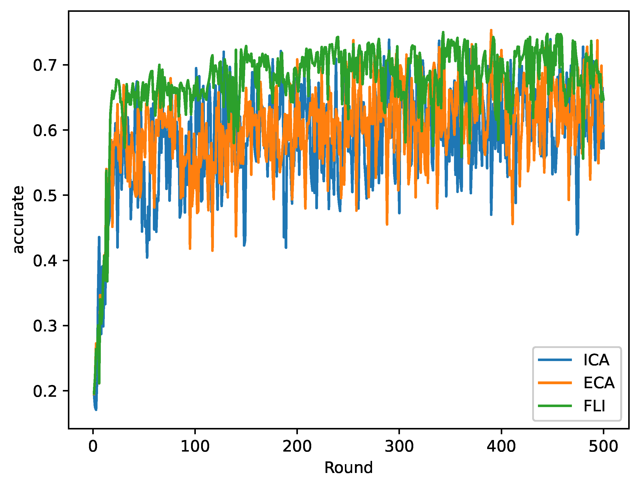
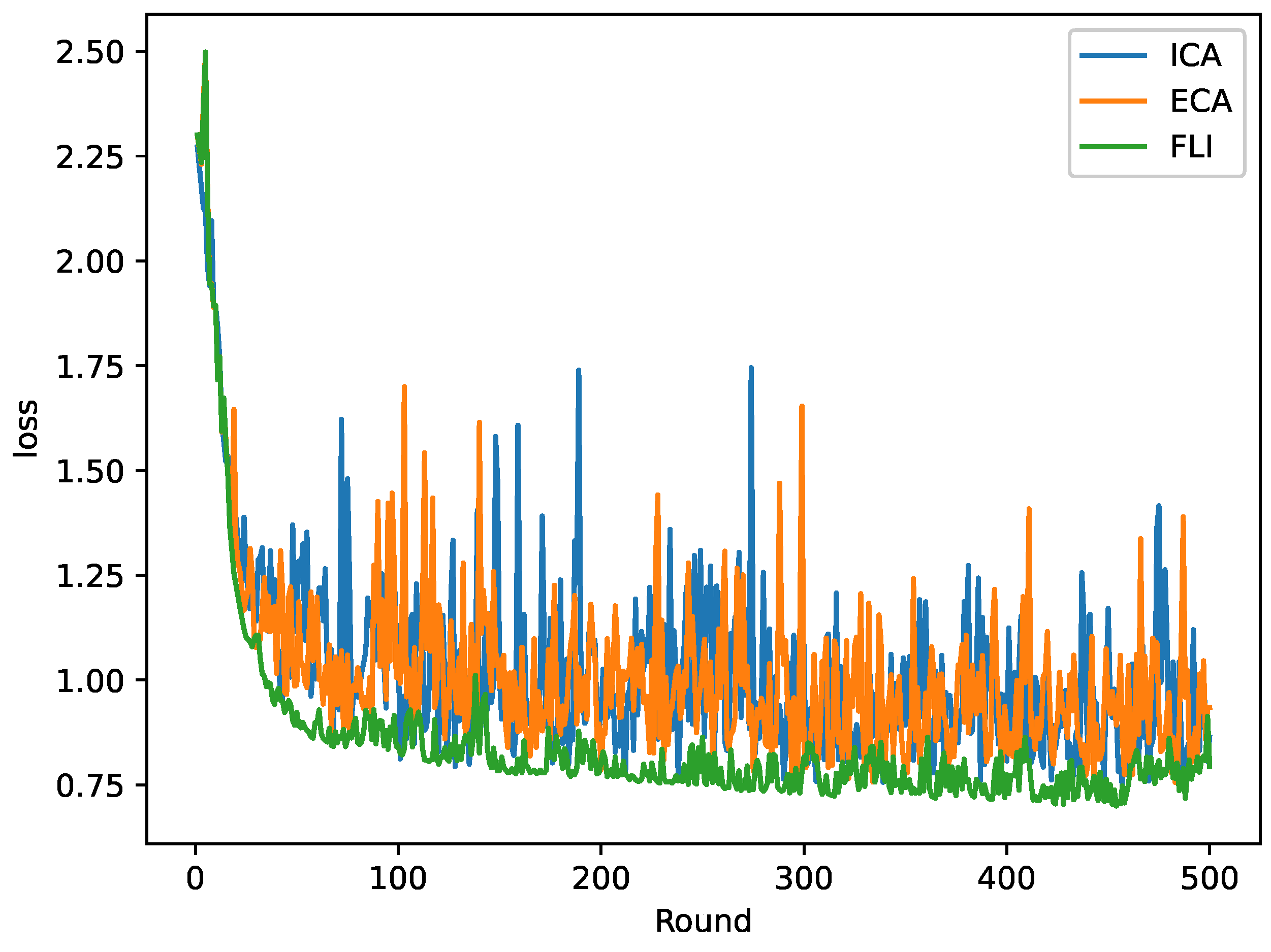
5.2. Results and Analysis

First, we compare the training performance of the FLI algorithm with the ECA and ICA in terms of training rounds (X-axis) versus training accuracy (Y-axis), as well as training rounds (X-axis) versus loss values (Y-axis). The results are illustrated in Figure 3 and Figure 4.

The experimental results indicate that our proposed algorithm achieves the best model training performance, requiring fewer communication rounds to reach higher training accuracy and lower loss. In contrast, both ECA and ICA exhibit similar performance, falling short of the effectiveness demonstrated by our algorithm. This suggests that Bayesian optimization facilitates more intelligent client selection by considering data complementarity and effective model updates. Meanwhile, the dynamic incentive mechanism adjusts incentives based on contributions, encouraging continuous participation from high-quality clients.

In contrast, although the ECA algorithm follows a fair and simple random selection strategy, it fails to effectively identify high-contribution clients. As a result, its model training performance is inferior to ours. Moreover, equal incentives may reduce the motivation of high-contribution clients, leading to lower long-term participation and impacting overall performance. ICA, on the other hand, relies on gradient evaluation, which may introduce bias due to the non-IID nature of the data. Some clients may exhibit large gradients but provide limited actual contributions, potentially leading to misallocated incentives that reward low-value clients and degrade the overall training outcome.

The reduction in training rounds not only shortens the overall training time but also brings significant energy efficiency benefits from a system-wide perspective. Specifically, the total energy consumption of the training process can be expressed as ${\sum }_{t=1}^T{E}_k\left(t\right)$, where T denotes the total number of communication rounds required for model convergence. Given that the central server is typically powered by a stable energy source while clients rely on limited battery resources, we focus on the energy expenditure at the edge, which is more sensitive to energy constraints. Thus, $E_k\left(t\right)$ is used to represent the energy consumed by client k in round t. As T decreases, the cumulative energy consumption at the edge correspondingly decreases, highlighting the efficiency advantage of our approach.

Next, we evaluated the training accuracy (Y-axis) of three algorithms under different incentive costs (X-axis). First, we compared ICA and FLI, setting ICA’s coefficient equal to $\beta$ at 0.01. Then, we tested ECA using the same total reward and training rounds as FLI. Therefore, we are able to compare the model training benefits achieved by FLI, ECA, and ICA under the same total incentive expenditure. The results are shown in Figure 5.

The results show that our proposed algorithm consistently outperforms both ICA and ECA under the same total incentive cost, achieving higher model accuracy and more efficient incentive utilization.

Unlike ECA and ICA, our method uses Bayesian prediction to estimate each client’s expected contribution based on past loss dynamics. This enables targeted incentive allocation to clients likely to contribute most in future rounds, reducing waste on low-impact participants. Additionally, our client selection strategy promotes diversity and complementarity, improving update representativeness and mitigating data heterogeneity.

ECA, in contrast, distributes incentives equally among randomly chosen clients without considering their actual utility. Though simple, it often selects low-quality participants, leading to inefficient resource use and poorer performance.

ICA improves on ECA by using gradient-based contribution estimates, but remains sensitive to noise and non-IID data. Gradient magnitudes can misrepresent client value, causing suboptimal incentive allocation. Moreover, ICA lacks a mechanism to predict future utility, limiting long-term optimization.

Finally, we repeat the experiment with four shards per client to evaluate the FLI algorithm under weak heterogeneity.

As can be seen from Figure 6, the FLI algorithm also shows good training performance when the heterogeneity is weak, achieving higher accuracy and more stable convergence with the same number of training rounds. Meanwhile, as heterogeneity decreases, the performance of the ICA also improves; athough it still lags behind our FLI algorithm, it clearly outperforms the ECA.

Next, we examine the impact of varying the number of participating clients per round on training performance. The results are presented in Figure 7 and Figure 8.

The results show that increasing the number of participating clients per round improves model performance. This is expected, as more clients provide access to a more diverse dataset, enhancing generalization, reducing overfitting, and accelerating convergence through more frequent parameter updates.

However, this improvement comes at a cost. As the number of participating clients increases, so does the total incentive expenditure, especially in incentive-aware federated learning frameworks where each selected client is compensated. This creates a trade-off between training performance and incentive efficiency, particularly under limited budgets or energy constraints.

Thus, while a larger client pool per round can enhance performance, it may not be optimal system-wide. Future work can explore dynamic strategies to determine the optimal number of participating clients, balancing performance gains and incentive costs.

Finally, we adjust the value of parameter $\beta$ to further investigate the impact of different incentive expenditure levels on the experimental results.

As shown in Figure 9, with the increase in $\beta$, the total incentive required to achieve the same training performance also increases. This observation is consistent with our experimental settings, where it is assumed that the incentives provided by the central server are sufficient to fully cover the clients’ energy consumption (as indicated in Equation (23)). Therefore, issues such as insufficient incentives due to a small $\beta$, which might lead to low client participation and degraded training performance, do not occur in our setup.

It is worth noting that our assumption is idealized, as clients in real-world deployments may expect more than just compensation for their energy costs; they often seek additional rewards to maintain high participation willingness. On the other hand, if $\beta$ is set too large, the total incentive expenditure increases significantly, as shown in the figure. This could rapidly exhaust the central server’s incentive budget, negatively affecting the continued training process.

In the rest of our experiments, we choose $\beta =0.01$ as a trade-off. This value avoids depleting the incentive budget while still offering sufficient incentives to ensure client participation. However, this work does not fully address the trade-off between incentive budget and client engagement. In future work, we plan to incorporate more practical constraints (such as total incentive budget and client participation willingness) to further explore the sensitivity and adaptability of $\beta$ under various application scenarios.

6. Discussion

This study proposes the FLI algorithm, which demonstrates superior training performance across various experimental scenarios. It is worth highlighting that, compared to the existing studies, this work effectively addresses the trade-off between efficiency and complexity in client selection. Prior methods have achieved impressive performance but often introduce substantial computational overhead, making them less suitable for resource-constrained scenarios. In contrast, the proposed loss-based client selection mechanism leverages naturally occurring training loss as the selection criterion, thereby avoiding additional communication and computational costs. This makes it particularly well-suited for real-time systems like intelligent traffic monitoring. Moreover, while most existing works treat incentive mechanisms and client selection as separate components, our approach tightly integrates the incentive allocation process with client selection. By incorporating Bayesian optimization, the proposed framework not only enhances model performance but also maintains system efficiency and fairness. In this regard, our work complements and extends the current literature by providing a lightweight, effective solution that is both theoretically sound and practically applicable.

However, the current approach assumes that the central server has a sufficient incentive budget, without fully considering the constraints of limited budgets or the variability in client participation willingness in real-world deployments. Moreover, the observed trade-off between the number of participating clients and incentive costs suggests that future work should further explore strategies for dynamically controlling client participation to achieve an optimal balance between training performance and system overhead.

While the use of the AWGN channel assumption simplifies the analysis and isolates the core aspects of client selection and incentive mechanisms, it may not fully capture the complexities of real-world communication environments. In practical scenarios, factors such as fading, interference, and Doppler shifts can significantly affect the communication performance and, in turn, influence the efficiency of client selection and model training. These channel impairments could lead to higher communication costs, reduced data reliability, and potential delays in model aggregation, all of which may impact the overall performance of the FLI algorithm. Therefore, future research should explore more realistic communication models to better understand how these factors interact with the proposed framework and to enhance its robustness in real-world deployments.

In real-world deployment, although the proposed air–ground collaborative federated learning framework offers theoretical advantages, the deployment of UAVs and UGVs will face several challenges. First, the flight altitude, route planning, and battery life of UAVs are significantly affected by external factors such as weather, wind speed, and temperature. Adverse weather conditions like strong winds or thunderstorms may cause UAVs to lose stability, affecting the continuity of data collection and transmission. UGVs, on the other hand, are constrained by ground environments, where road conditions, traffic congestion, or obstacles may impact their inspection efficiency. Moreover, in the dynamic urban traffic environment, UAVs and UGVs need to cope with complex scenario changes, including road construction and temporary traffic control, all of which can affect monitoring accuracy and real-time performance. Therefore, future deployment will not only require further optimization of algorithms to improve the robustness and flexibility of the system but also need to account for how to adapt to the constantly changing external environment to ensure the stability and efficient operation of the system.

7. Future Work

In future work, we plan to extend the FLI algorithm to more realistic deployment scenarios characterized by constrained or dynamically changing incentive budgets. To enhance its practical applicability, we will incorporate real-time budget management and proactive incentive strategies based on the prediction of client participation willingness, inferred from historical behavior and contextual information. Furthermore, we will explore adaptive client population control mechanisms that dynamically regulate the number of participating clients according to system load, budget constraints, and performance objectives, thereby optimizing the trade-off between model performance and resource consumption. In addition, we aim to account for complex and dynamic communication environments—such as rain fading, multipath propagation, and UAV node failures—that may result in unstable links, transmission interruptions, and reduced client availability.

8. Conclusions

This paper proposes an air–ground collaborative federated learning framework for smart city traffic monitoring, which leverages the capabilities of unmanned aerial vehicles (UAVs) and unmanned ground vehicles (UGVs) to achieve efficient data collection and model training. The framework employs Bayesian optimization for client selection based on client contributions and designs an incentive mechanism based on these contributions, ensuring high model performance while minimizing the total incentive cost. Simulation experiments demonstrate that, compared to the traditional client selection algorithms, the proposed method accelerates model convergence and effectively reduces incentive costs. This research contributes to improving the efficiency, sustainability, and adaptability of smart city traffic management systems by addressing key challenges such as privacy protection, resource optimization, and client participation. Future work will focus on expanding the framework to address dynamic incentive budgets and complex communication environments, ensuring its practical application in real-world urban traffic monitoring systems.

References

1. Kopetz, H.; Steiner, W. Internet of things. In Real-Time Systems: Design Principles for Distributed Embedded Applications; Springer: Cham, Switzerland, 2022; pp. 325–341. [Google Scholar]
2. Bello, O.; Zeadally, S. Intelligent device-to-device communication in the internet of things. IEEE Syst. J. 2014, 10, 1172–1182. [Google Scholar] [CrossRef]
3. Tien, J.M. Internet of things, real-time decision making, and artificial intelligence. Ann. Data Sci. 2017, 4, 149–178. [Google Scholar] [CrossRef]
4. Motlagh, N.H.; Taleb, T.; Arouk, O. Low-altitude unmanned aerial vehicles-based internet of things services: Comprehensive survey and future perspectives. IEEE Internet Things J. 2016, 3, 899–922. [Google Scholar] [CrossRef]
5. Qiu, J.; Grace, D.; Ding, G.; Zakaria, M.D.; Wu, Q. Air-ground heterogeneous networks for 5G and beyond via integrating high and low altitude platforms. IEEE Wirel. Commun. 2019, 26, 140–148. [Google Scholar] [CrossRef]
6. Wang, J.; Shao, Y.; Ge, Y.; Yu, R. A survey of vehicle to everything (V2X) testing. Sensors 2019, 19, 334. [Google Scholar] [CrossRef]
7. Tong, W.; Hussain, A.; Bo, W.X.; Maharjan, S. Artificial intelligence for vehicle-to-everything: A survey. IEEE Access 2019, 7, 10823–10843. [Google Scholar] [CrossRef]
8. Seo, H.; Lee, K.D.; Yasukawa, S.; Peng, Y.; Sartori, P. LTE evolution for vehicle-to-everything services. IEEE Commun. Mag. 2016, 54, 22–28. [Google Scholar] [CrossRef]
9. Yin, Y.; Liu, M.; Gui, G.; Gacanin, H.; Sari, H. Minimizing delay for MIMO-NOMA resource allocation in UAV-assisted caching networks. IEEE Trans. Veh. Technol. 2022, 72, 4728–4732. [Google Scholar] [CrossRef]
10. Nellore, K.; Hancke, G.P. A survey on urban traffic management system using wireless sensor networks. Sensors 2016, 16, 157. [Google Scholar] [CrossRef]
11. Liu, J.; Shi, Y.; Fadlullah, Z.M.; Kato, N. Space-air-ground integrated network: A survey. IEEE Commun. Surv. Tutor. 2018, 20, 2714–2741. [Google Scholar] [CrossRef]
12. Yin, Y.; Gui, G.; Liu, M.; Gacanin, H.; Sari, H.; Adachi, F. Joint User pairing and resource allocation in air-to-ground communication-caching-charging integrated network based on NOMA. IEEE Trans. Veh. Technol. 2023, 72, 15819–15828. [Google Scholar] [CrossRef]
13. Chen, Q.; Meng, W.; Li, S.; Li, C.; Chen, H.H. Civil aircrafts augmented space–air–ground-integrated vehicular networks: Motivation, breakthrough, and challenges. IEEE Internet Things J. 2021, 9, 5670–5683. [Google Scholar] [CrossRef]
14. Cheng, N.; Xu, W.; Shi, W.; Zhou, Y.; Lu, N.; Zhou, H.; Shen, X. Air-ground integrated mobile edge networks: Architecture, challenges, and opportunities. IEEE Commun. Mag. 2018, 56, 26–32. [Google Scholar] [CrossRef]
15. Buch, N.; Velastin, S.A.; Orwell, J. A review of computer vision techniques for the analysis of urban traffic. IEEE Trans. Intell. Transp. Syst. 2011, 12, 920–939. [Google Scholar] [CrossRef]
16. Zhao, D.; Dai, Y.; Zhang, Z. Computational intelligence in urban traffic signal control: A survey. IEEE Trans. Syst. Man Cybern. Part C (Appl. Rev.) 2011, 42, 485–494. [Google Scholar] [CrossRef]
17. Zhang, Y.; Chen, D.; Wang, S.; Tian, L. A promising trend for field information collection: An air-ground multi-sensor monitoring system. Inf. Process. Agric. 2018, 5, 224–233. [Google Scholar] [CrossRef]
18. Barrado, C.; Messeguer, R.; López, J.; Pastor, E.; Santamaria, E.; Royo, P. Wildfire monitoring using a mixed air-ground mobile network. IEEE Pervasive Comput. 2010, 9, 24–32. [Google Scholar] [CrossRef]
19. Valente, J.; Sanz, D.; Barrientos, A.; Del Cerro, J.; Ribeiro, Á.; Rossi, C. An air-ground wireless sensor network for crop monitoring. Sensors 2011, 11, 6088–6108. [Google Scholar] [CrossRef]
20. Nigam, N.; Singh, D.P.; Choudhary, J. A review of different components of the intelligent traffic management system (ITMS). Symmetry 2023, 15, 583. [Google Scholar] [CrossRef]
21. Latif, S.; Afzaal, H.; Zafar, N.A. Intelligent traffic monitoring and guidance system for smart city. In Proceedings of the 2018 International Conference on Computing, Mathematics and Engineering Technologies (iCoMET), Sukkur, Pakistan, 3–4 March 2018; pp. 1–6. [Google Scholar]
22. Jordan, S.; Moore, J.; Hovet, S.; Box, J.; Perry, J.; Kirsche, K.; Lewis, D.; Tse, Z.T.H. State-of-the-art technologies for UAV inspections. IET Radar Sonar Navig. 2018, 12, 151–164. [Google Scholar] [CrossRef]
23. Mentsiev, A.U.; Guzueva, E.R.; Magomaev, T.R. Security challenges of the Industry 4.0. J. Phys. Conf. Ser. 2020, 1515, 032074. [Google Scholar] [CrossRef]
24. Zhou, Z.; Zhang, C.; Xu, C.; Xiong, F.; Zhang, Y.; Umer, T. Energy-efficient industrial internet of UAVs for power line inspection in smart grid. IEEE Trans. Ind. Inform. 2018, 14, 2705–2714. [Google Scholar] [CrossRef]
25. Zhang, C.; Xie, Y.; Bai, H.; Yu, B.; Li, W.; Gao, Y. A survey on federated learning. Knowl.-Based Syst. 2021, 216, 106775. [Google Scholar] [CrossRef]
26. Liu, M.; Xia, Y.; Zhao, H.; Guo, L.; Shi, Z.; Zhu, H. Federated Learning Technologies for 6G Industrial Internet of Things: From Requirements, Vision to Challenges, Opportunities. J. Electron. Inf. Technol. 2024, 46, 4335–4353. [Google Scholar]
27. Bonawitz, K.; Eichner, H.; Grieskamp, W.; Huba, D.; Ingerman, A.; Ivanov, V.; Kiddon, C.; Konečnỳ, J.; Mazzocchi, S.; McMahan, B.; et al. Towards federated learning at scale: System design. Proc. Mach. Learn. Syst. 2019, 1, 374–388. [Google Scholar]
28. Zhao, H.; Shi, Y.; Liu, M.; Zhu, H.; Xun, W. Fairness Can Save Lives: A MAB based Client Selection Strategy for Federated Learning towards IoV assisted ITS. IEEE Trans. Veh. Technol. 2024, 74, 5430–5441. [Google Scholar] [CrossRef]
29. Kairouz, P.; McMahan, H.B.; Avent, B.; Bellet, A.; Bennis, M.; Bhagoji, A.N.; Bonawitz, K.; Charles, Z.; Cormode, G.; Cummings, R.; et al. Advances and open problems in federated learning. Found. Trends® Mach. Learn. 2021, 14, 1–210. [Google Scholar] [CrossRef]
30. Zhan, Y.; Zhang, J.; Hong, Z.; Wu, L.; Li, P.; Guo, S. A survey of incentive mechanism design for federated learning. IEEE Trans. Emerg. Top. Comput. 2021, 10, 1035–1044. [Google Scholar] [CrossRef]
31. Zhao, H.; Sui, M.; Liu, M.; Zhu, C.; Xun, W.; Xu, B.; Zhu, H. Are You Diligent, Inefficient, or Malicious? A Self-Safeguarding Incentive Mechanism for Large Scale-Federated Industrial Maintenance Based on Double Layer Reinforcement Learning. IEEE Internet Things J. 2024, 11, 19988–20001. [Google Scholar] [CrossRef]
32. Zeng, R.; Zeng, C.; Wang, X.; Li, B.; Chu, X. A comprehensive survey of incentive mechanism for federated learning. arXiv 2021, arXiv:2106.15406. [Google Scholar]
33. Asad, M.; Moustafa, A.; Rabhi, F.A.; Aslam, M. THF: 3-way hierarchical framework for efficient client selection and resource management in federated learning. IEEE Internet Things J. 2021, 9, 11085–11097. [Google Scholar] [CrossRef]
34. Qu, Z.; Duan, R.; Chen, L.; Xu, J.; Lu, Z.; Liu, Y. Context-aware online client selection for hierarchical federated learning. IEEE Trans. Parallel Distrib. Syst. 2022, 33, 4353–4367. [Google Scholar] [CrossRef]
35. Wang, Y.; Su, Z.; Luan, T.H.; Li, R.; Zhang, K. Federated learning with fair incentives and robust aggregation for UAV-aided crowdsensing. IEEE Trans. Netw. Sci. Eng. 2021, 9, 3179–3196. [Google Scholar] [CrossRef]
36. Chen, C.; Gong, S.; Zhang, W.; Zheng, Y.; Kiat, Y.C. DRL-based contract incentive for wireless-powered and UAV-assisted backscattering MEC system. IEEE Trans. Cloud Comput. 2024, 12, 264–276. [Google Scholar] [CrossRef]
37. Xie, L.; Su, Z.; Chen, N.; Xu, Q. Secure data sharing in UAV-assisted crowdsensing: Integration of blockchain and reputation incentive. In Proceedings of the 2021 IEEE Global Communications Conference (GLOBECOM), Madrid, Spain, 7–11 December 2021; pp. 1–6. [Google Scholar]
38. Kang, J.; Xiong, Z.; Niyato, D.; Xie, S.; Zhang, J. Incentive mechanism for reliable federated learning: A joint optimization approach to combining reputation and contract theory. IEEE Internet Things J. 2019, 6, 10700–10714. [Google Scholar] [CrossRef]
39. Chabrol, M.; Sarramia, D.; Tchernev, N. Urban traffic systems modelling methodology. Int. J. Prod. Econ. 2006, 99, 156–176. [Google Scholar] [CrossRef]
40. Abbasi, M.; Shahraki, A.; Taherkordi, A. Deep learning for network traffic monitoring and analysis (NTMA): A survey. Comput. Commun. 2021, 170, 19–41. [Google Scholar] [CrossRef]
41. Liu, M.; Lin, W.; Wang, Q.; Gui, G. Survey on Data Heterogeneity Problems and Personalization Based Solutions of Federated Learning in Internet of Vehicles. J. Commun. 2024, 45, 207–224. [Google Scholar]
42. Zhao, Y.; Li, M.; Lai, L.; Suda, N.; Civin, D.; Chandra, V. Federated learning with non-iid data. arXiv 2018, arXiv:1806.00582. [Google Scholar] [CrossRef]
43. Wu, Q.; Zhang, R. Common throughput maximization in UAV-enabled OFDMA systems with delay consideration. IEEE Trans. Commun. 2018, 66, 6614–6627. [Google Scholar] [CrossRef]
44. Albaseer, A.; Abdallah, M.; Al-Fuqaha, A.; Erbad, A. Client Selection Approach in Support of Clustered Federated Learning over Wireless Edge Networks. In Proceedings of the 2021 IEEE Global Communications Conference (GLOBECOM), Madrid, Spain, 7–11 December 2021; pp. 1–6. [Google Scholar] [CrossRef]
45. Tang, M.; Ning, X.; Wang, Y.; Sun, J.; Wang, Y.; Li, H.; Chen, Y. FedCor: Correlation-based active client selection strategy for heterogeneous federated learning. In Proceedings of the IEEE/CVF Conference on Computer Vision and Pattern Recognition, New Orleans, LA, USA, 18–24 June 2022; pp. 10102–10111. [Google Scholar]
46. Sheng, Y.; Zeng, L.; Cao, S.; Dai, Q.; Yang, S.; Lu, J. FedBoost: Bayesian Estimation Based Client Selection for Federated Learning. IEEE Access 2024, 12, 52255–52266. [Google Scholar] [CrossRef]
47. McMahan, B.; Moore, E.; Ramage, D.; Hampson, S.; y Arcas, B.A. Communication-efficient learning of deep networks from decentralized data. In Proceedings of the Artificial Intelligence and Statistics. PMLR, Fort Lauderdale, FL, USA, 20–22 April 2017; pp. 1273–1282. [Google Scholar]
48. Shi, Y.; Yu, H.; Leung, C. Towards Fairness-Aware Federated Learning. IEEE Trans. Neural Netw. Learn. Syst. 2024, 35, 11922–11938. [Google Scholar] [CrossRef] [PubMed]
49. Li, J.; Chen, T.; Teng, S. A comprehensive survey on client selection strategies in federated learning. Comput. Netw. 2024, 251, 110663. [Google Scholar] [CrossRef]
Figure 1. Schematic of urban traffic monitoring scenario.
Electronics 14 01891 g001
Figure 2. Federated learning flowchart.
Electronics 14 01891 g002
Figure 3. Comparison of training accuracy versus training rounds for the three algorithms.
Electronics 14 01891 g003
Figure 4. Comparison of training loss versus training rounds for the three algorithms.
Electronics 14 01891 g004
Figure 5. Comparison of training performance versus incentive cost for the three algorithms.
Electronics 14 01891 g005
Figure 6. Algorithm accuracy comparison when shards per client is set to 4.
Electronics 14 01891 g006
Figure 7. Comparison of training accuracy versus training rounds for different numbers of participating clients.
Electronics 14 01891 g007
Figure 8. Comparison of training loss versus training rounds for different numbers of participating clients.
Electronics 14 01891 g008
Figure 9. Comparison of training accuracy versus incentive cost for different β .
Electronics 14 01891 g009