Commonness and Inconsistency Learning with Structure Constrained Adaptive Loss Minimization for Multi-View Clustering

Abstract

Subspace clustering has emerged as a prominent research focus, demonstrating remarkable potential in handling multi-view data by effectively harnessing their diverse and information-rich features. In this study, we present a novel framework for multi-view subspace clustering that addresses several critical aspects of the problem. Our approach introduces three key innovations: First, we propose a dual-component representation model that simultaneously considers both consistent and inconsistent elements across different views. The consistent component is designed to capture shared structural patterns with robust commonality, while the inconsistent component effectively models view-specific variations through sparsity constraints across multiple modes. Second, we implement cross-mode sparsity constraints that enable the inconsistent component to efficiently extract high-order information from the data. This design not only enhances the representation capability of the inconsistent component but also facilitates the consistent component in revealing high-order structural relationships within the data. Third, we develop an adaptive loss function that offers greater flexibility in handling noise and outliers, thereby significantly improving the model’s robustness in real-world applications. Through extensive experimentation, we demonstrate that our proposed method consistently outperforms existing approaches, achieving superior clustering performance across various benchmark datasets. The experimental results comprehensively validate the effectiveness and advantages of our approach in terms of clustering accuracy, robustness, and computational efficiency.

1. Introduction

As a basic approach in machine learning, clustering has proven to be highly effective in diverse areas, including image segmentation [1], face clustering [2], community detection [3], cancer biology [4], text mining [5], etc. High-dimensional data often contain redundant or irrelevant features that can obscure meaningful patterns, making traditional clustering methods less effective. By reducing dimensionality, innovative techniques help to reveal the underlying structure of the data, improving both the efficiency and accuracy of clustering algorithms. Thus, there has been an ongoing requirement to develop innovative techniques, such as low-dimensional representations [6,7,8], for clustering that can elucidate the latent structures within high-dimensional data.

Subspace clustering has been well studied during the last decades with great success in constructing low-dimensional representations for efficient clustering [1,7,9,10,11]. Among them, the subspace clustering methods built upon spectral clustering principles have attracted considerable interest and become the focus of recent developments in subspace clustering methods [6,7,12]. The sparse subspace clustering [13] and low-rank representation [7] approaches are among the most typical methods. Various algorithms have been developed with improved clustering performance [12,14]. However, in practical applications, data often originate from various sources [15]. As an example, we can utilize various features such as texts, images, or other types of characteristics to depict an object [15]. These features are considered as multi-view representations of the object, providing a comprehensive and diverse perspective on the data and resulting in multi-view data. Although multi-view data offer richer and more informative information than single-view data, single-view methods are unable to effectively utilize the features available across multiple views and thus they may have suboptimal learning performance.

To tackle this challenge, multi-view clustering techniques have been thoroughly investigated over the past decade, yielding promising clustering performance [16,17,18,19,20]. Existing methods can be broadly categorized into two types based on their approach to constructing the affinity matrix [21], which are briefly summarized in Figure 1. The first type constructs the affinity matrix directly from similarity matrices [16,17,18,22], while the second type, known as multi-view subspace clustering, builds on spectral clustering-based subspace clustering techniques [15,19,23]. For instance, LT-MSC extends the traditional low-rank representation framework by incorporating a tensor nuclear norm constraint to explore cross-view correlations and global structures [24]. Similarly, CSMSC emphasizes both consistency and specificity in representations, enabling the identification of shared and view-specific characteristics [25]. Another notable method, MLRR, improves low-rank representation by applying symmetry constraints and diversity regularization to preserve angular consistency and capture view-specific information [26]. MVCIL tackles catastrophic forgetting and concept interference in open-ended incremental learning via random representation, orthogonal fusion, and selective weight consolidation [27]. The EOMSC-CA method integrates anchor learning and graph construction, and by imposing graph connectivity constraints, it directly outputs clustering labels [28].

Despite these advancements, existing methods still face several critical limitations. First, many approaches fail to effectively exploit the cross-view high-order information and spatial structure of the data, resulting in incomplete representations that do not well capture the underlying relationships across views. Second, while consistency and diversity across views are crucial for multi-view clustering, current methods often struggle to balance these aspects, leading to either over-emphasis on shared structures or neglect of view-specific characteristics. Third, the robustness of existing methods to noise and outliers remains a challenge, as many approaches rely on rigid loss functions that are sensitive to data imperfections.

To address these limitations, we propose a novel multi-view clustering method that integrates consistency and diversity across views while capturing high-order information and enhancing robustness. Our approach introduces the following key innovations: (1) We adopt an adaptive loss function that combines the benefits of various matrix norms. This strategy effectively mitigates the effects of noise and outliers, and thus makes the proposed model more robust. (2) We separate the representation matrix of each view into two parts that correspond to consistency and inconsistency of the data, respectively. In particular, the consistency part exhibits the desired structural property with strict commonality and block diagonal structural constraints, which enhances the affinity matrix to explicitly identify the grouping pattern of the data. Meanwhile, the inconsistency part captures high-order information of the data through sparsity constraints imposed on different modes. This strategy effectively helps reveal latent cross-view structures of the data. (3) The proposed model involves several terms, which are complicated and not straightforward to solve. We design an effective optimization algorithm for the proposed method, which generalizes the practical applicability of the proposed techniques. (4) Through extensive experimental results, the effectiveness and superiority of our method have been effectively demonstrated, which further improves the learning performance of the MVC algorithms.

The rest of this paper is organized as follows: Section 2 introduces the essential background information. In Section 3, we introduce the proposed method, followed by the development of an optimization algorithm in Section 4. In Section 5, we perform comprehensive experiments to confirm the efficacy of the proposed method. Finally, we summarize the findings and conclude the paper in Section 6.

2. Background Knowledge

Herein, we introduce the required notations and offer a concise review of related methods. Given multi-view data $\mathbf{X}$, we denote its number of samples by n, number of views by V, number of clusters by k, dimension of each view by $d_v$ with $v=1,\dots ,V$, and the largest dimension is $d=Ma{x}_{v=1}^V\left\{d_v\right\}$. We represent the feature matrix for each view as ${\mathbf{X}}^{\left(v\right)}\in {\mathbb{R}}^{d_v\times n}$. For ease of notation, the superscript ${(·)}^{\left(v\right)}$ is also used to denote the v-th frontal slice of the tensors. Subsequently, a self-expression-based multi-view subspace clustering model can be universally formulated as follows:

$$\underset{{\mathit{Ƶ}}^{\left(1\right)},\cdots ,{\mathit{Ƶ}}^{\left(V\right)}}{min}\mathcal{G}({\mathbf{X}}^{\left(v\right)},{\mathbf{X}}^{\left(v\right)}{\mathit{Ƶ}}^{\left(v\right)})+\tau \psi \left({\mathit{Ƶ}}^{\left(v\right)}\right),$$

(1)

where tensor $\mathit{Ƶ}\in {\mathcal{R}}^{n\times n\times V}$ consists of representation matrices in each frontal slice, $\mathcal{G}(·)$ serves as the loss function of ${\mathit{Ƶ}}^{\left(v\right)}$, $\tau \ge 0$ serves as a balancing parameter, and $\psi (·)$ functions as a regularizer of ${\mathit{Ƶ}}^{\left(v\right)}$. When $V=1$, the aforementioned model simplifies to a traditional single-view subspace clustering method like the tensor nuclear norm and low-rank representation, while employing their respective regularizers.

3. Proposed Method

In general, utilizing the self-expressive property allows us to formulate the multi-view clustering model as

$$\begin{array}{cc}\hfill & \underset{\mathit{Ƶ}}{min}\sum _{v=1}^V{\parallel {\mathbf{X}}^{\left(v\right)}-{\mathbf{X}}^{\left(v\right)}{\mathit{Ƶ}}^{\left(v\right)}\parallel }_F^2+f\left(\mathit{Ƶ}\right),\hfill \end{array}$$

(2)

where $f\left(\mathit{Ƶ}\right)$ denotes a proper regularizer for the affinity tensor. This regularizer enforces constraints on the structural characteristics of the low-dimensional representation within each individual view. Generally, when a model is fitted using the samples, most of the samples lead to a small loss while a big loss is generated by only a few samples [29].

To alleviate the loss function’s sensitivity to outliers, as well as to marry the advantages of different norms, for enhanced robustness and accurate information preservation from the data, we adopt an adaptive loss function [29]. In particular, for an arbitrary matrix $\mathbf{A}\in {\mathbb{R}}^{a\times b}$, the adaptive loss function can be formulated as follows:

$${∥\mathbf{A}∥}_{\sigma }=\sum _i{\displaystyle \frac{(1+\sigma ){∥{\mathbf{A}}^i∥}_2^2}{{∥{\mathbf{A}}^i∥}_2+\sigma }}$$

(3)

where the i-th row of the matrix $\mathbf{A}$ is denoted by ${\mathbf{A}}^i$ and $\sigma >0$ is a parameter. The adaptive loss function is closely related to various matrix norms, of which the properties are summarized in lemmaadaptive.

Lemma 1

([29]). For matrix $\mathbf{A}\in {\mathbb{R}}^{a\times b}$, the following are the characteristics of the adaptive loss function:

1.

The norm ${∥\mathbf{A}∥}_{\sigma }$ is nonnegative and convex.

2.

The norm ${∥\mathbf{A}∥}_{\sigma }$ is twice differentiable.

3.

If $\forall i\in \{1,\cdots ,a\}$, $\parallel {\mathbf{A}}^i{\parallel }_{\sigma }\ll \sigma$, then ${∥\mathbf{A}∥}_{\sigma }\to {\displaystyle \frac{(1+\sigma )}{\sigma }}{∥\mathbf{A}∥}_F^2$.

4.

If $\forall i\in \{1,\cdots ,a\}$, ${∥{\mathbf{A}}^i∥}_{\sigma }\gg \sigma$, then ${∥\mathbf{A}∥}_{\sigma }\to (1+\sigma ){∥\mathbf{A}∥}_{2,1}$, where ${∥\mathbf{A}∥}_{2,1}={\sum }_{i=1}^m{\left({\sum }_{\mathbf{J}=1}^n{A}_{i\mathbf{J}}^2\right)}^{1/2}$.

5.

$\underset{\sigma \to 0}{lim}{∥\mathbf{A}∥}_{\sigma }\to {∥\mathbf{A}∥}_{2,1}$.

6.

$\underset{\sigma \to \infty }{lim}{∥\mathbf{X}∥}_{\sigma }\to {∥\mathbf{X}∥}_F^2$.

Thus, with the adaptive loss function, we may develop Equation (2) into

$$\begin{array}{cc}\hfill & \underset{\mathit{Ƶ}}{min}\sum _{v=1}^V{\parallel {\mathbf{X}}^{\left(v\right)}-{\mathbf{X}}^{\left(v\right)}{\mathit{Ƶ}}^{\left(v\right)}\parallel }_{\sigma }+f\left(\mathit{Ƶ}\right).\hfill \end{array}$$

(4)

In general, different views of the data exhibit both consistency and inconsistency, where the consistency reflects the shared information across all views, while the inconsistency captures the unique diversity information of each view. To effectively capture the consistency and inconsistency information of the representation matrices among different views, we follow and decompose the representation tensor $\mathit{Ƶ}$ into consistent and inconsistent parts as $\mathit{Ƶ}=\mathcal{C}+\mathcal{E}$ [30], which are captured by $\mathcal{C}\in {\mathbb{R}}^{n\times n\times V}$ and $\mathcal{E}\in {\mathbb{R}}^{n\times n\times V}$, respectively. In this paper, we aim to assist in capturing the strong commonalities among different views, and we propose to extract a common part from the multiple representation matrices, which is denoted as $\mathbf{C}\in {\mathbb{R}}^{n\times n}$. Thus, each view’s representation matrix can be factorized as ${\mathit{Ƶ}}^{\left(v\right)}=\mathbf{C}+{\mathcal{E}}^{\left(v\right)}$ with a hard commonness constraint. Therefore, we may further develop Equation (4) into

$$\begin{array}{cc}\hfill & \underset{\mathbf{C},\mathcal{E}}{min}\sum _{v=1}^V{\parallel {\mathbf{X}}^{\left(v\right)}-{\mathbf{X}}^{\left(v\right)}(\mathbf{C}+{\mathcal{E}}^{\left(v\right)})\parallel }_{\sigma }+g(\mathbf{C},\mathcal{E}),\hfill \end{array}$$

(5)

where $g(\mathbf{C},\mathcal{E})$ serves as an appropriate regularizer to enforce the desired structural properties of both $\mathbf{C}$ and $\mathcal{E}$. In general, it is expected that the inconsistency of different views should not be significantly large since different views have close connections, which suggests that $\mathcal{E}$ is sparse. To enhance the sparse structures of the inconsistency part, we consider the following two cases. First, the sample-wise sparsity has been widely considered, which leads to mode-2 sparsity of $\mathcal{E}$. Second, for each sample, the representation vectors in different views should be similar, which leads to a mode-3 sparse structure of $\mathcal{E}$. Thus, to ensure that $\mathcal{E}$ has a joint mode-2 and mode-3 sparse structure, we further develop Equation (5) into

$$\begin{array}{cc}\hfill & \underset{\mathbf{C},\mathcal{E}}{min}\sum _{v=1}^V{\parallel {\mathbf{X}}^{\left(v\right)}-{\mathbf{X}}^{\left(v\right)}(\mathbf{C}+{\mathcal{E}}^{\left(v\right)})\parallel }_{\sigma }+\alpha \left\{\sum _{ij}{\left(\sum _v{\mathcal{E}}_{ijv}^2\right)}^{1/2}+\sum _{jv}{\left(\sum _i{\mathcal{E}}_{ijv}^2\right)}^{1/2}\right\},\hfill \end{array}$$

(6)

where $\alpha$ is a balancing parameter. Although the sparsity of $\mathcal{E}$ helps capture the commonness across different views to construct $\mathbf{C}$, we still need to exploit the structural constraint for $\mathbf{C}$ for the desired structural properties of the common representation. First, it is natural to impose structural constraints on the consensus affinity matrix, which gives rise to

$$\begin{array}{cc}\hfill & \underset{\mathbf{C},\mathcal{E}}{min}\sum _{v=1}^V{\parallel {\mathbf{X}}^{\left(v\right)}-{\mathbf{X}}^{\left(v\right)}(\mathbf{C}+{\mathcal{E}}^{\left(v\right)})\parallel }_{\sigma }+\alpha \left\{\sum _{ij}{\left(\sum _v{\mathcal{E}}_{ijv}^2\right)}^{1/2}+\sum _{jv}{\left(\sum _i{\mathcal{E}}_{ijv}^2\right)}^{1/2}\right\},\hfill \\ \hfill & s.t.\mathrm{diag}\left(\mathbf{C}\right)=0,\mathbf{C}\ge 0,\mathbf{C}={\mathbf{C}}^{\top },\hfill \end{array}$$

(7)

where $\mathrm{diag}(·)$ extracts the diagonal elements of the input matrix and arranges them into a column vector. The constraints imposed in Equation (7) require that $\mathbf{C}$ is nonnegative and symmetric and avoid a trivial interpretation of $\mathbf{C}$ that the coefficient of a sample itself is the largest by restricting $\mathrm{diag}\left(\mathbf{C}\right)=0$, which enforces the natural and desired property for an affinity matrix. To further exploit the local and nonlinear structures inherent in the data, we introduce the graph Laplacian to our model, which leads to

$$\begin{array}{cc}\hfill & \underset{\mathbf{C},\mathcal{E}}{min}\sum _{v=1}^V{\parallel {\mathbf{X}}^{\left(v\right)}-{\mathbf{X}}^{\left(v\right)}(\mathbf{C}+{\mathcal{E}}^{\left(v\right)})\parallel }_{\sigma }+\alpha \left\{\sum _{ij}{\left(\sum _v{\mathcal{E}}_{ijv}^2\right)}^{1/2}+\sum _{jv}{\left(\sum _i{\mathcal{E}}_{ijv}^2\right)}^{1/2}\right\}\hfill \\ \hfill & +\beta \sum _{v=1}^V\mathbf{Tr}\left(\mathbf{C}{\mathcal{L}}^{\left(v\right)}{\mathbf{C}}^{\top }\right),s.t.\mathrm{diag}\left(\mathbf{C}\right)=0,\mathbf{C}\ge 0,\mathbf{C}={\mathbf{C}}^{\top },\hfill \end{array}$$

(8)

where $\beta$ serves the role of a balancing parameter and $\mathcal{L}\in {\mathbb{R}}^{n\times n\times V}$ denotes a tensor that consists of graph Laplacian matrices of different views in frontal slices. It is seen that the manifold learning embedded in the third term of Equation (8) provides a consensus local geometric structure of $\mathbf{C}$ across different views, which is important in revealing the structures of the data [31]. The structural constraints naturally treat $\mathbf{C}$ as a graph matrix, which measures neighbor relationships of the data. For such data, the connected components are k, each corresponding to a distinct cluster.

To guarantee such property, we refer to the theorem stated below.

Theorem 1 

([32]). For any $\mathbf{C}\ge 0$ and ${\mathbf{C}}^{\top }=\mathbf{C}$, let $\mathbb{L}\left(\mathbf{C}\right)$ be its Laplacian matrix. The number of connected components present in $\mathbf{C}$ is reflected by the multiplicity k of the eigenvalue 0 of ${\mathbb{L}}_{\mathbf{C}}$.

Theorem 1 inspires us to restrict that $\mathbb{L}\left(\mathbf{C}\right)$ has exactly k zero eigenvalues for the desired connectivity property of $\mathbf{C}$. It is straightforward to impose constraint $\mathbf{Rank}\left(\mathbb{L}\right(\mathbf{C}\left)\right)$ into Equation (7) to restrict the rank of $\mathbb{L}\left(\mathbf{C}\right)$, with $\mathbf{Rank}(·)$ being the rank operator. However, it is widely recognized that this problem, which involves rank minimization, is NP-hard [32], making it challenging to solve. Thus, we refer to the following k-block diagonal regularizer for a relaxed rank constraint.

Definition 1 

([14]). Given an affinity matrix $\mathbf{B}\in {\mathbb{R}}^{n\times n}$, a k-block diagonal regularizer can be defined as

$$\begin{array}{c}\hfill {∥\mathbf{B}∥}_k=\sum _{i=n-k+1}^n{\lambda }_i\left(\mathbb{L}\left(\mathbf{B}\right)\right),\end{array}$$

(9)

where ${\lambda }_i(·)$ denotes the matrix singular value of the input and is the i-th largest.

It is seen that the k-block diagonal regularizer can be treated as a relaxed rank constraint, by minimizing which we may ideally restrict the desired rank for the target graph Laplacian matrix. Then, $\mathbf{C}$ ideally contains k connected sub-graphs, which correspond to the k clusters of the data and thus reveal the group structure of the data. Thus, with the connectivity constraint of $\mathbf{C}$, we further develop our model as

$$\begin{array}{cc}\hfill & \underset{\mathbf{C},\mathcal{E}}{min}\sum _{v=1}^V{\parallel {\mathbf{X}}^{\left(v\right)}-{\mathbf{X}}^{\left(v\right)}(\mathbf{C}+{\mathcal{E}}^{\left(v\right)})\parallel }_{\sigma }+\beta \sum _{v=1}^V\mathbf{Tr}\left(\mathbf{C}{\mathcal{L}}^{\left(v\right)}{\mathbf{C}}^{\top }\right)\hfill \\ \hfill & +\alpha \left\{\sum _{ij}{\left(\sum _v{\mathcal{E}}_{ijv}^2\right)}^{1/2}+\sum _{jv}{\left(\sum _i{\mathcal{E}}_{ijv}^2\right)}^{1/2}\right\}+\gamma {\parallel \mathbf{C}\parallel }_k,\hfill \\ \hfill & s.t.\mathrm{diag}\left(\mathbf{C}\right)=0,\mathbf{C}\ge 0,\mathbf{C}={\mathbf{C}}^{\top },\hfill \end{array}$$

(10)

where $\gamma$ is a balancing parameter. The aforementioned model is named Commonness and Inconsistency Learning with Structure Constrained Adaptive Loss Minimization for Multi-view Clustering (CISCAL-MVC). We summarize the flow diagram of the CISCAL-MVC in Figure 2. We will present an effective optimization algorithm to address Equation (10) in the next section.

4. Optimization

In this section, we will develop an effective optimization algorithm for Equation (10) by employing the augmented Lagrange multiplier method (ALM). First, we introduce several auxiliary variables to facilitate the optimization and construct the augmented Lagrange function. Then, our algorithm efficiently solves the optimization problem by decomposing it into several manageable subproblems. For all the subproblems, we provide their corresponding closed-form solutions using various techniques, such as the Sylvester equation, shrinkage operator, etc. We update each of the variables while fixing the others till convergence. The detailed optimization procedure is presented as follows:

Since the fourth term is highly nonlinear and difficult to solve, we convert it to an equivalent form to facilitate the optimization. First, we may refer to the following Theorem 2 as a useful tool.

Theorem 2 

([33]). ∀$\mathbf{L}\in {\mathbb{R}}^{n\times n}$ and $\mathbf{L}⪰0,$ the following equality holds:

$$\sum _{i=n-k+1}^n{\lambda }_i\left(\mathbf{L}\right)=inf\left\{\langle \mathbf{L},\mathbf{W}\rangle |\mathbf{W}\in {\mathbb{R}}^{n\times n},0⪯\mathbf{W}⪯\mathbf{I},\mathbf{Tr}\left(\mathbf{W}\right)=k\right\},$$

(11)

where $\langle ·\rangle$ denotes the inner product of matrices.

Then, according to Definition 1 and Theorem 2, we may rewrite ${\parallel \mathbf{C}\parallel }_k$ as the following convex programming problem:

$$\begin{array}{c}\hfill \underset{\mathbf{W}\in {\mathbb{R}}^{n\times n},0⪯\mathbf{W}⪯\mathbf{I},\mathbf{Tr}\left(\mathbf{W}\right)=k}{min}\langle \mathbb{L}\left(\mathbf{C}\right),\mathbf{W}\rangle .\end{array}$$

(12)

Thus, we may convert the original objective into an equivalent form as follows:

$$\begin{array}{cc}\hfill & \underset{\mathbf{C},\mathcal{E},\mathbf{W}}{min}\sum _{v=1}^V\parallel {\mathbf{X}}^{\left(v\right)}-{\mathbf{X}}^{\left(v\right)}(\mathbf{C}+{\mathcal{E}}^{\left(v\right)}){\parallel }_{\sigma }\hfill \\ \hfill & +\alpha \left\{\sum _{ij}{\left(\sum _v{\mathcal{E}}_{ijv}^2\right)}^{1/2}+\sum _{jv}{\left(\sum _i{\mathcal{E}}_{ijv}^2\right)}^{1/2}\right\},\hfill \\ \hfill & +\beta \sum _{v=1}^V\mathbf{Tr}\left(\mathbf{C}{\mathcal{L}}^{\left(v\right)}{\mathbf{C}}^{\top }\right)+\gamma \langle \mathrm{Diag}\left(\mathbf{C}1\right)-\mathbf{C}),\mathbf{W}\rangle \hfill \\ \hfill & s.t.\mathrm{diag}\left(\mathbf{C}\right)=0,\mathbf{C}\ge 0,\mathbf{C}={\mathbf{C}}^{\top },0⪯\mathbf{W}⪯\mathbf{I},\mathbf{Tr}\left(\mathbf{W}\right)=k,\hfill \end{array}$$

(13)

where $\mathrm{Diag}(·)$ denotes an operator that transforms the input vector into a diagonal matrix. To solve Equation (13), we first introduce auxiliary variables $\mathbf{J}=\mathbf{C}\in {\mathbb{R}}^{n\times n}$ and $\mathcal{S}=\mathcal{F}=\mathcal{E}\in {\mathbb{R}}^{n\times n\times V}$. Then, the augmented Lagrange function of equation Equation (13) can be expressed as

$$\begin{array}{cc}\hfill & L(\mathbf{J},\mathbf{C},\mathcal{E},\mathcal{F},\mathcal{S})=\sum _{v=1}^V\parallel {\mathbf{X}}^{\left(v\right)}-{\mathbf{X}}^{\left(v\right)}(\mathbf{J}+{\mathcal{S}}^{\left(v\right)}){\parallel }_{\sigma }\hfill \\ \hfill & +\alpha \left\{\sum _{ij}{\left(\sum _v{\mathcal{E}}_{ijv}^2\right)}^{1/2}+\sum _{jv}{\left(\sum _i{\mathcal{F}}_{ijv}^2\right)}^{1/2}\right\}+\beta \sum _{v=1}^V\mathbf{Tr}\left(\mathbf{J}{\mathcal{L}}^{\left(v\right)}{\mathbf{J}}^{\top }\right)\hfill \\ \hfill & +\gamma \langle \mathrm{Diag}\left(\mathbf{C}1\right)-\mathbf{C}),\mathbf{W}\rangle +{\displaystyle \frac{\mu }{2}}{\parallel \mathbf{J}-\mathbf{C}+\mathbf{Y}/\mu \parallel }_F^2\hfill \\ \hfill & +{\displaystyle \frac{\mu }{2}}\parallel {\mathcal{S}}^{\left(v\right)}-{\mathcal{E}}^{\left(v\right)}+{\mathcal{Y}}_1^{\left(v\right)}{/\mu \parallel }_F^2+{\displaystyle \frac{\mu }{2}}{\parallel {\mathcal{F}}^{\left(v\right)}-{\mathcal{E}}^{\left(v\right)}+{\mathcal{Y}}_2^{\left(v\right)}/\mu \parallel }_F^2,\hfill \\ \hfill & s.t.\mathrm{diag}\left(\mathbf{C}\right)=0,\mathbf{C}\ge 0,\mathbf{C}={\mathbf{C}}^{\top },0⪯\mathbf{W}⪯\mathbf{I},\mathbf{Tr}\left(\mathbf{W}\right)=k,\hfill \end{array}$$

(14)

where the Lagrange multipliers are given by $\mathbf{Y}\in {\mathbb{R}}^{n\times n}$, ${\mathcal{Y}}_1\in {\mathbb{R}}^{n\times n\times V}$, and ${\mathcal{Y}}_2\in {\mathbb{R}}^{n\times n\times V}$, and the penalty parameter of the ALM is given by $\mu$, respectively.

4.1. $\mathit{J}$-Subproblem

The subproblem connected with J is

$$\begin{array}{cc}\hfill & \underset{\mathbf{J}}{\min }\sum _{v=1}^V\parallel {\mathbf{X}}^{\left(v\right)}-{\mathbf{X}}^{\left(v\right)}(\mathbf{J}+{\mathcal{S}}^{\left(v\right)}){\parallel }_{\sigma }+\beta \sum _{v=1}^V\mathbf{Tr}\left(\mathbf{J}{\mathcal{L}}^{\left(v\right)}{\mathbf{J}}^{\top }\right)+{\displaystyle \frac{\mu }{2}}{\parallel {\mathbf{J}}^{(-)}\mathbf{C}+\mathbf{Y}/\mu \parallel }_F^2.\hfill \end{array}$$

(15)

Define $\mathcal{H}\in {\mathbb{R}}^{n\times n\times V}$ and $\mathcal{D}\in {\mathbb{R}}^{n\times n\times V}$ with ${\mathcal{H}}^{\left(v\right)}={\mathcal{S}}^{\left(v\right)}-\mathbf{I} \mathrm{and} {\mathcal{D}}_{i\mathbf{J}}^{\left(v\right)}={\mathbb{I}}_{\{i=\mathbf{J}\}}·(1+\sigma )·{\displaystyle \frac{\parallel {\left({\mathbf{X}}^{\left(v\right)}\right)}^i(\mathbf{J}+{\mathcal{H}}^{\left(v\right)}){\parallel }_2+2\sigma }{2(\parallel {\left({\mathbf{X}}^{\left(v\right)}\right)}^i(\mathbf{J}+{\mathcal{H}}^{\left(v\right)}){{\parallel }_2+\sigma )}^2}},$ then Equation (15) can be restructured as:

$$\begin{gathered} \begin{array}{cc}\hfill & \underset{\mathrm{J}}{\min }\sum _{v=1}^V\mathbf{Tr}\left({\mathcal{D}}^{\left(v\right)}{\mathbf{X}}^{\left(v\right)}({\mathcal{H}}^{\left(v\right)}+\mathbf{J}({\mathcal{H}}^{\left(v\right)}+{\mathbf{J}}^{\top }{\left({\mathbf{X}}^{\left(v\right)}\right)}^{\top }\right) \\ +\beta \sum _{v=1}^V\mathbf{Tr}\left(\mathbf{J}{\mathcal{L}}^{\left(v\right)}{\mathbf{J}}^{\top }\right)+{\displaystyle \frac{\mu }{2}}{\parallel \mathbf{J}-\mathbf{C}+\mathbf{Y}/\mu \parallel }_F^2.\hspace{1em}\hspace{1em}\hspace{1em}\hspace{1em}\hfill \end{array} \end{gathered}$$

(16)

The above problem appears complicated in J and is not straightforward to solve. To facilitate the optimization, we first reformulate the above problem into the following form:

$$\begin{gathered} \begin{array}{c}\hfill \begin{array}{cc}\hfill & \underset{\mathbf{J}}{min}\mathbf{Tr}\left({\mathbf{J}}^{\top }\left(\sum _{v=1}^V{\left({\mathbf{X}}^{\left(v\right)}\right)}^{\top }{\mathcal{D}}^{\left(v\right)}{\mathbf{X}}^{\left(v\right)}\right)\mathbf{J}\right)+2\mathbf{Tr}\left({\mathbf{J}}^{\top }\sum _{v=1}^V{\left({\mathbf{X}}^{\left(v\right)}\right)}^{\top }{\mathcal{D}}^{\left(v\right)}{\mathbf{X}}^{\left(v\right)}{\mathcal{H}}^{\left(v\right)}\right) \\ +\beta \mathbf{Tr}\left(\mathbf{J}\sum _{v=1}^V{\mathcal{L}}^{\left(v\right)}{\mathbf{J}}^{\top }\right)+{\displaystyle \frac{\mu }{2}}{\parallel \mathbf{J}-\mathbf{C}+\mathbf{Y}/\mu \parallel }_F^2.\hspace{1em}\hspace{1em}\hspace{1em}\hspace{1em}\hspace{1em}\hspace{1em}\hspace{1em}\hspace{1em}\hspace{1em}\hspace{1em}\hspace{1em}\hfill \end{array}\end{array} \end{gathered}$$

(17)

To ensure that the above problem has a minimizer, we need to show that the above problem is convex. For the first term, it is seen that $\forall \nu \in {\mathbb{R}}^n \mathrm{and} \nu \ne 0,$ the following inequality holds:

$$\begin{array}{c}\hfill \begin{array}{cc}\hfill & {\nu }^{\top }\left(\sum _{v=1}^V{\left({\mathbf{X}}^{\left(v\right)}\right)}^{\top }{\mathcal{D}}^{\left(v\right)}{\mathbf{X}}^{\left(v\right)}\right)\nu \hfill \\ \hfill =& \sum _{v=1}^V{\nu }^{\top }{\left({\mathbf{X}}^{\left(v\right)}\right)}^{\top }{\mathcal{D}}^{\left(v\right)}{\mathbf{X}}^{\left(v\right)}\nu \hfill \\ \hfill =& \sum _{v=1}^V{\nu }^{\top }{\left({\mathbf{X}}^{\left(v\right)}\right)}^{\top }{\left({\left({\mathcal{D}}^{\left(v\right)}\right)}^{1/2}\right)}^{\top }{\left({\mathcal{D}}^{\left(v\right)}\right)}^{1/2}{\mathbf{X}}^{\left(v\right)}\nu \hfill \\ \hfill =& \sum _{v=1}^V{\parallel {\left({\mathcal{D}}^{\left(v\right)}\right)}^{1/2}{\mathbf{X}}^{\left(v\right)}\nu \parallel }_2^2\ge 0,\hfill \end{array}\end{array}$$

(18)

which confirms the convexity of the first term of Equation (17). Since ${\mathcal{L}}^{\left(v\right)}$ is the graph Laplacian matrix constructed from ${\mathbf{X}}^{\left(v\right)},$ we have ${\mathcal{L}}^{\left(v\right)}⪰0$ and thus $\sum _{v=1}^V{\mathcal{L}}^{\left(v\right)}⪰0$ as well [31]. Moreover, it is clear that the second term of Equation (17) is linear while the last term is quadratic. Then, it is clear that Equation (16) is quadratic and convex, which can be solved by the first-order optimality condition:

$$\begin{array}{c}\hfill \begin{array}{cc}\hfill & \sum _{v=1}^V\left(2{\left({\mathbf{X}}^{\left(v\right)}\right)}^{\top }{\mathcal{D}}^{\left(v\right)}{\mathbf{X}}^{\left(v\right)}\right)·\mathbf{J}+\mathbf{J}·2\beta \sum _{v=1}^V{\mathcal{L}}^{\left(v\right)}\hfill \\ \hfill & +\sum _{v=1}^{V}2{\left({\mathbf{X}}^{\left(v\right)}\right)}^{\top }{\mathcal{D}}^{\left(v\right)}{\mathbf{X}}^{\left(v\right)}{\mathcal{H}}^{\left(v\right)}+\mu \mathbf{J}+\mathbf{Y}-\mu \mathbf{C}=0.\hfill \end{array}\end{array}$$

(19)

The above equation is essentially a Sylvester equation. To be clearer, we define:

$$\begin{array}{cc}\hfill {\Theta }_1& :=2\sum _{v=1}^V{\left({\mathbf{X}}^{\left(v\right)}\right)}^{\top }{\mathcal{D}}^{\left(v\right)}{\mathbf{X}}^{\left(v\right)}+\mu \mathbf{I},\hfill \\ \hfill {\Theta }_2& :=2\beta \sum _{v=1}^V{\mathcal{L}}^{\left(v\right)},\hfill \\ \hfill {\Theta }_3& :=\sum _{v=1}^{V}2{\left({\mathbf{X}}^{\left(v\right)}\right)}^{\top }{\mathcal{D}}^{\left(v\right)}{\mathbf{X}}^{\left(v\right)}{\mathcal{H}}^{\left(v\right)}-\mu \mathbf{C}+\mathbf{Y}.\hfill \end{array}$$

(20)

Then, by plugging Equation (20) into Equation (19), we obtain a standard Sylvester equation as follows:

$$\begin{array}{c}\hfill {\Theta }_1\mathbf{J}+\mathbf{J}{\Theta }_2+{\Theta }_3=0.\end{array}$$

(21)

For the Sylvester equation in Equation (21), we may adopt various algorithms such as the Bartels–Stewart [34] or the Hessenberg–Schur [35] algorithm to efficiently resolve the problem, which generally requires $\mathcal{O}\left(n^3\right)$ complexity. It is noted that we may also apply other algorithms, such as the gradient descent, to the original optimization problem of Equation (17). By using the gradient, we need to obtain the gradient of the objective at each iteration, which requires $\mathcal{O}\left(n^3\right)$ complexity. The Sylvester equation solver directly addresses the first-order optimality conditions, typically achieving an exact solution in a finite number of steps, making it highly efficient and numerically stable for small to medium-scale problems. In contrast, gradient descent relies on iterative updates, often exhibiting slower convergence, particularly for ill-conditioned problems, leading to potential robustness issues. Without loss of generality, we adopt the Sylvester equation solver and summarize the above steps as the following operator:

$$\mathbf{J}=\mathbf{Sylvester}({\Theta }_1,{\Theta }_2,{\Theta }_3).$$

(22)

4.2. $\mathit{C}$-Subproblem

The subproblem for $\mathbf{C}$ is presented as follows:

$$\begin{array}{cc}\hfill & \underset{\mathbf{C}}{min}\gamma \langle \mathrm{Diag}\left(\mathbf{C}1\right)-\mathbf{C}),\mathbf{W}\rangle +{\displaystyle \frac{\mu }{2}}{\parallel \mathbf{J}-\mathbf{C}+\mathbf{Y}/\mu \parallel }_F^2\hfill \\ \hfill & s.t.\mathrm{diag}\left(\mathbf{C}\right)=0,\mathbf{C}\ge 0,\mathbf{C}={\mathbf{C}}^{\top }.\hfill \end{array}$$

(23)

With straightforward algebra, the aforementioned problem can be reformulated equivalently as

$$\begin{array}{cc}\hfill & \underset{\mathbf{C}}{min}{∥\mathbf{C}-\mathbf{J}-{\displaystyle \frac{\mathbf{Y}-\gamma ·\mathrm{diag}\left(\mathbf{W}\right){\mathbf{1}}^{\top }+\gamma \mathbf{W}}{\mu }}∥}_F^2,\hfill \\ \hfill & s.t.\mathrm{diag}\left(\mathbf{C}\right)=0,\mathbf{C}\ge 0,\mathbf{C}={\mathbf{C}}^{\top }.\hfill \end{array}$$

(24)

For ease of notation, we define

$$\overline{\mathbf{C}}:=\mathbf{J}+{\displaystyle \frac{\mathbf{Y}-\gamma ·\mathrm{diag}\left(\mathbf{W}\right){\mathbf{1}}^{\top }+\gamma \mathbf{W}}{\mu }}.$$

Then, according to [14], Equation (24) admits a closed-form solution:

$$\begin{array}{c}\hfill \mathbf{C}={\left({\displaystyle \frac{\overline{\mathbf{C}}+{\overline{\mathbf{C}}}^{\top }}{2}}-\mathrm{Diag}\left(\mathrm{diag}\left(\overline{\mathbf{C}}\right)\right)\right)}_{+},\end{array}$$

(25)

where ${(·)}_{+}$ denotes the nonnegative projection.

4.3. $\mathit{W}$-Subproblem

The subproblem of $\mathbf{W}$ is as follows:

$$\begin{array}{cc}\hfill & \underset{0⪯\mathbf{W}⪯\mathbf{I},\mathbf{Tr}\left(\mathbf{W}\right)=k}{min}\langle \mathrm{Diag}\left(\mathbf{C}1\right)-\mathbf{C}),\mathbf{W}\rangle .\hfill \end{array}$$

(26)

According to [36], Equation (26) admits a closed-form solution:

$$\mathbf{W}={\mathbf{PP}}^{\top },$$

(27)

where the eigenvectors of $\mathbb{L}\left(\mathbf{C}\right)$ corresponding to the smallest k eigenvalues are represented by $\mathbf{P}$.

4.4. $\mathcal{S}$-Subproblem

The subproblem associated with $\mathcal{S}$ is as follows:

$$\begin{array}{cc}\hfill \underset{\mathcal{S}}{min}& \sum _{v=1}^V\parallel {\mathbf{X}}^{\left(v\right)}-{\mathbf{X}}^{\left(v\right)}(\mathbf{J}+{\mathcal{S}}^{\left(v\right)}){\parallel }_{\sigma }+{\displaystyle \frac{\mu }{2}}{\parallel \mathcal{S}-\mathcal{E}+{\mathcal{Y}}_1/\mu \parallel }_F^2.\hfill \end{array}$$

(28)

In a way similar to Equation (16), we may rewrite the above problem into:

$$\begin{array}{cc}\hfill \underset{\mathcal{S}}{min}& \sum _{v=1}^V\mathbf{Tr}\left({(\mathbf{J}-\mathbf{I}+{\mathcal{S}}^{\left(v\right)})}^{\top }{\left({\mathbf{X}}^{\left(v\right)}\right)}^{\top }{\mathcal{D}}^{\left(v\right)}{\mathbf{X}}^{\left(v\right)}(\mathbf{J}-\mathbf{I}+{\mathcal{S}}^{\left(v\right)})\right)\hfill \\ \hfill & +{\displaystyle \frac{\mu }{2}}{\parallel \mathcal{S}-\mathcal{E}+{\mathcal{Y}}_1/\mu \parallel }_F^2.\hfill \end{array}$$

(29)

It is evident that Equation (29) can be solved by slice. For each ${\mathcal{S}}^{\left(v\right)}$, it is clear that the corresponding problem is quadratic and convex, and a closed-form solution can be obtained by the first-order optimality condition:

$$\begin{array}{c}\hfill 2{\left({\mathbf{X}}^{\left(v\right)}\right)}^{\top }{\mathcal{D}}^{\left(v\right)}{\mathbf{X}}^{\left(v\right)}(\mathbf{J}-\mathbf{I}+{\mathcal{S}}^{\left(v\right)})+\mu ({\mathcal{S}}^{\left(v\right)}-{\mathcal{E}}^{\left(v\right)}+{\mathcal{Y}}_1^{\left(v\right)}/\mu )=0.\end{array}$$

(30)

Thus, $\mathcal{S}$ can be obtained by slice as

$$\begin{array}{cc}\hfill {\mathcal{S}}^{\left(v\right)}=& {\left(2{\left({\mathbf{X}}^{\left(v\right)}\right)}^{\top }{\mathcal{D}}^{\left(v\right)}{\mathbf{X}}^{\left(v\right)}+\mu \mathbf{I}\right)}^{-1}\hfill \\ \hfill & ·\left(\mu {\mathcal{E}}^{\left(v\right)}-{\mathcal{Y}}_1^{\left(v\right)}-2{\left({\mathbf{X}}^{\left(v\right)}\right)}^{\top }{\mathcal{D}}^{\left(v\right)}{\mathbf{X}}^{\left(v\right)}(\mathbf{J}-\mathbf{I})\right).\hfill \end{array}$$

(31)

4.5. $\mathcal{E}$-Subproblem

For $\mathcal{E}$, the subproblem is:

$$\begin{array}{cc}\hfill \underset{\mathcal{E}}{min}\alpha & \sum _{ij}{\left(\sum _v{\mathcal{E}}_{ijv}^2\right)}^{1/2}+{\displaystyle \frac{\mu }{2}}{\parallel {\mathcal{S}}^{\left(v\right)}-{\mathcal{E}}^{\left(v\right)}+{\mathcal{Y}}_1^{\left(v\right)}/\mu \parallel }_F^2\hfill \\ \hfill & +{\displaystyle \frac{\mu }{2}}{\parallel {\mathcal{F}}^{\left(v\right)}-{\mathcal{E}}^{\left(v\right)}+{\mathcal{Y}}_2^{\left(v\right)}/\mu \parallel }_F^2.\hfill \end{array}$$

(32)

The above problem is essentially a ${\ell }_{2,1}$-shrinkage problem of $\mathcal{E}$ along the mode-3 fiber, which can be clearly seen by a simplified standard form in the following:

$$\begin{array}{cc}\hfill \underset{\mathcal{E}}{min}& {\displaystyle \frac{\alpha }{2\mu }}\sum _{ij}{\left(\sum _v{\mathcal{E}}_{ijv}^2\right)}^{1/2}+{\displaystyle \frac{1}{2}}\parallel {\mathcal{E}}^{\left(v\right)}-{\displaystyle \frac{{\mathcal{S}}^{\left(v\right)}+{\mathcal{F}}^{\left(v\right)}+{\mathcal{Y}}_1^{\left(v\right)}/\mu +{\mathcal{Y}}_2^{\left(v\right)}/\mu }{2}}{\parallel }_F^2.\hfill \end{array}$$

(33)

Then, according to [37], Equation (33) admits a closed-form solution along the mode-3 fiber as follows:

$${\mathcal{E}}_{ijv}={\displaystyle \frac{{\left({\sum }_{v^{\prime }=1}^V{\widehat{\mathcal{E}}}_{ij{v}^{\prime }}^2\right)}^{1/2}-\frac{\alpha }{2\mu }}{{\left({\sum }_{v^{\prime }=1}^V{\widehat{\mathcal{E}}}_{ij{v}^{\prime }}^2\right)}^{1/2}}}·{\widehat{\mathcal{E}}}_{ijv}·{\mathbb{I}}_{\{{\left({\sum }_{v^{\prime }=1}^V{\widehat{\mathcal{E}}}_{ij{v}^{\prime }}^2\right)}^{1/2}>{\displaystyle \frac{\alpha }{2\mu }}\}},$$

(34)

where $\widehat{\mathcal{E}}={\displaystyle \frac{\mathcal{S}+\mathcal{F}+{\mathcal{Y}}_1/\mu +{\mathcal{Y}}_2/\mu }{2}}$, and ${\mathbb{I}}_{\{·\}}$ is a function that returns 0 if it does not satisfy the condition in the subscript and returns 0 if it does.

4.6. $\mathcal{F}$-Subproblem

For $\mathcal{F}$, the subproblem is

$$\begin{array}{c}\hfill \underset{\mathcal{F}}{min}\alpha \sum _{jv}{\left(\sum _i{\mathcal{F}}_{ijv}^2\right)}^{1/2}+{\displaystyle \frac{\mu }{2}}{\parallel \mathcal{F}-\mathcal{E}+{\mathcal{Y}}_2/\mu \parallel }_F^2.\end{array}$$

(35)

Similarly to Equation (32), the aforementioned problem can be solved using the ${\ell }_{2,1}$-shrinkage operator; so, we have the following closed-form solution:

$${\mathcal{F}}_{ijv}={\displaystyle \frac{{\left({\sum }_{i^{\prime }=1}^n{\widehat{\mathcal{F}}}_{i^{\prime }jv}^2\right)}^{1/2}-\frac{\alpha }{\mu }}{{\left({\sum }_{i^{\prime }=1}^n{\widehat{\mathcal{F}}}_{i^{\prime }jv}^2\right)}^{1/2}}}·{\widehat{\mathcal{F}}}_{ijv}·{\mathbb{I}}_{\{{\left({\sum }_{i^{\prime }=1}^n{\widehat{\mathcal{F}}}_{i^{\prime }jv}^2\right)}^{1/2}>{\displaystyle \frac{\alpha }{\mu }}\}},$$

(36)

where $\mathcal{F}=\mathcal{E}-{\mathcal{Y}}_2/\mu$.

4.7. Updating of $\mathit{Y}$,${\mathcal{Y}}_{\mathbf{1}}$, ${\mathcal{Y}}_{\mathbf{2}}$, and μ

We update the Lagrange multiplier and penalty parameters using classical methods, as outlined below:

$$\begin{array}{cc}\hfill \mathbf{Y}& =\mathbf{Y}+\mu (\mathbf{J}-\mathbf{C}),\hfill \\ \hfill {\mathcal{Y}}_1& ={\mathcal{Y}}_1+\mu (\mathcal{S}-\mathcal{E}),\hfill \\ \hfill {\mathcal{Y}}_2& ={\mathcal{Y}}_2+\mu (\mathcal{F}-\mathcal{E}),\hfill \\ \hfill \mu & =\mu \kappa ,\hfill \end{array}$$

(37)

where $\kappa >1$ keeps that $\mu$ is increasing. We iterate the above steps until convergence is achieved, then we may obtain a unified view-commonness matrix $\mathbf{C}$. Finally, we apply standard spectral clustering techniques to $\mathbf{C}$ to achieve the final clustering result.

4.8. Time Complexity

We analyze the time complexity of our method as follows. In particular, we analyze the dominant operations that determine the complexity of our algorithm at each iteration. For the J-subproblem, it needs to solve a Sylvester equation, which requires a time complexity of $\mathcal{O}(V{n}^{2}d+n^3)$ by utilizing the Bartels–Stewart algorithm [34]. For the C-subproblem, it requires a time complexity $\mathcal{O}\left(n^3\right)$. The time complexity for constructing graph Laplacian matrices is $\mathcal{O}\left(n^3\right)$. Similarly to J, the W-subproblem requires a time complexity of $\mathcal{O}(V{n}^2+n^{2}n)$ for calculating the matrix multiplications and solving the Sylvester equations. For the $\mathcal{S}$-subproblem, it has a similar structure to J and requires a time complexity of $\mathcal{O}(V{n}^3+V{n}^2{d}_v)$. Regarding the subproblems of $\mathcal{E}$ and $\mathcal{F}$, both entail l_2,1 norm contraction operations, leading to a time complexity of $\mathcal{O}\left(V{n}^2\right)$ for each. In summary, it requires a total time complexity of $\mathcal{O}(V{n}^3+V{n}^{2}d+n^{2}k)$.

5. Experiments

In this section, experiments are carried out to validate the effectiveness of our method. Especially, we compare our method with nine baseline methods, which will be introduced in the following subsection. Six datasets are utilized, including the 3Sources [38], ORL [39], WebKB-Texas [40], COIL-20 [41], Caltech-7 [42], and Yale [43] datasets. We adopt four evaluation metrics—the clustering accuracy (ACC) as a measure of cluster assignment correctness, normalized mutual information (NMI) as an indication of clustering quality, purity (PUR) as a metric for cluster homogeneity, and the adjusted rand index (ARI) as a measure of clustering agreement—whose details can be found in [44,45,46,47,48]. Basically, the first three metrics values range within [0, 1] while the last one is within [−1, 1], where the larger value indicates better performance. All experiments in this paper are conducted using MATLAB 2018a on a workstation equipped with a 6-core Intel i5-8500T CPU running at 2.10 GHz and 16 GB of memory. The detailed experimental setup, along with the corresponding results, is presented in the subsequent parts of this section. The code for our method can be accessed on 28 March 2025, at https://www.researchgate.net/profile/Chong-Peng-8/publications.

5.1. Methods in Comparison

In the experiment, we conduct a comparison between our approach and nine other baseline methods: (1) SC [49] is a traditional clustering technique for single-view data. In our experiment, we execute SC independently on each view and present the optimal results; (2) MVSpec [50] extends the SC for multi-view data, which uses a weighted combination of kernel matrices of different views for clustering; (3) RMSC [22] constructs probability matrices from different views and learns a unified probability matrix with low-rank constraint for multi-view clustering; (4) MVGL [17] creates a unified graph by integrating affinity graphs from various views under a low-rank constraint, which is utilized for multi-view clustering; (5) BMVC [46] performs binary learning for representation and clustering; (6) SMVSC [11] performs anchor learning collaboratively and builds a unified graph to represent the underlying structures of the data; (7) MVSC [51] constructs a unified bipartite graph for clustering based on cross-view sample-anchor bipartite graphs; (8) FPMVS-CAG [52] introduces a parameter-free method that aims to obtain an anchor representation by combining anchor selection with graph construction for clustering; (9) JSMC [30] concurrently integrates the cross-view commonness and inconsistencies into the learning of subspace representations. (10) MvDSCN [53] learns a multi-view self-representation matrix in an end-to-end manner by integrating multiple backbones and combining convolutional autoencoders with self-representation.

5.2. Datasets

In our experiment, we utilize six benchmark datasets. The main features of these datasets are outlined in

Table 1. Overview of benchmark datasets.

Datasets	k	V	n	Dim. of Each View (${\mathit{d}}_{\mathit{v}}$)
				View 1	View 2	View 3
3Sources	6	3	169	3068	3631	3560
ORL	40	3	400	4096	6750	3304
WebKB-Texas	4	2	187	187	1703	$--$
COIL-20	20	3	1440	1024	3304	6750
Caltech-7	7	3	1474	512	1984	928
Yale	15	3	165	4096	3304	6750

, and we briefly introduce them as follows: (1) 3Sources [38] comprises data from 948 news articles. Each article presents multiple points of view and is drawn from three online news platforms: BBC, Reuters, and the Guardian. We only select the instances that have complete information across all views. The feature dimensions of the three news platforms are 3068d, 3631d, and 3560d, respectively. (2) ORL [39] contains 400 facial images of 40 individuals. The images were captured under various lighting conditions, showcasing a variety of facial expressions and intricate details. Three types of features, including the 4096d intensity, 6750d Gabor, and 3304d LBP, are preserved in this dataset. (3) WebKB-Texas [40] consists of 187 documents from the University of Texas Department of Computer Science homepage. These documents belong to five categories, including student, project, course, staff, and faculty. Each document has two types of features, including 187d citation and 1703d content. (4) COIL-20 [41] consists of 1440 grayscale images of 20 objects. For each object, 72 images are captured from different angles. Three types of features are preserved in this dataset, including the 1024d intensity, 3304d LBP, and 6750d Gabor. (5) Caltech-7 [42] selects 7 out of a total number of 101 classes from the Caltech-101 dataset, including Faces, Garfield, Snoopy, StopSign, Windsor-Chair, Dollar Bill, and Motorbikes. This dataset contains three types of features, including 512d GIST, 1984d HOG, and 928d LBP. (6) Yale [43] consists of 165 facial images of 15 persons. These images are captured with varying facial expressions under different lighting conditions. There are three types of features in this dataset, including 4096d intensity, 6750d Gabor, and 3304d LBP. We visually show some examples of the image datasets in Figure 3.

5.3. Clustering Performance

For all methods in the comparison, we utilize a grid search strategy for parameter tuning in the experiment. For our method, we adjust the balancing parameters $\alpha$, $\beta$, and $\gamma$ from the set ${\mathbb{S}}_1=\{{10}^{-3},{10}^{-2},\cdots ,{10}^3\}$, with the parameter $\sigma$ within the set ${\mathbb{S}}_2=\{1,2,3,\cdots ,10\}$, respectively. For the baseline methods, if not otherwise clarified in the original paper, we tune the balancing parameters within ${\mathbb{S}}_1$ as well. For each method, we enumerate all possible combinations of parameter values on each dataset and record the highest result for each evaluation metric, respectively. The clustering results are presented in detail in

Table 2. Comparison of clustering performance across various methods on benchmark datasets.

Dataset	3Sources				ORL				WebKB-Texas
Method	ACC	NMI	ARI	PUR	ACC	NMI	ARI	PUR	ACC	NMI	ARI	PUR
SC	48.52	38.69	20.81	59.17	77.25	89.12	69.75	80.00	57.75	29.36	23.91	69.52
MVSpec	25.44	6.610	00.85	39.64	19.50	39.42	1.980	21.25	32.09	10.15	−4.640	55.08
RMSC	62.54	58.56	48.87	76.33	70.23	84.79	61.42	74.31	48.64	26.01	18.51	68.80
MVGL	35.50	8.070	−0.720	40.24	72.00	82.96	38.79	77.75	51.87	6.550	2.480	57.22
BMVC	65.68	58.69	54.32	73.37	16.75	39.29	00.61	18.00	56.68	24.73	25.18	68.98
SMVSC	31.36	8.920	4.000	44.38	56.25	75.26	42.39	60.25	56.25	21.42	29.01	67.91
MVSC	75.85	66.48	58.38	80.89	72.36	84.69	56.59	77.05	55.13	1.980	0.190	56.10
FPMVS-CAG	26.04	6.590	42.60	1.010	56.00	74.63	39.99	60.00	57.75	22.76	29.81	65.78
JSMC	77.51	69.52	65.17	82.25	82.00	91.46	77.79	84.50	73.33	38.04	32.26	70.05
MvDSCN	77.24	68.29	61.35	81.21	87.25	1.01	82.98	81.06	57.62	28.14	28.19	68.86
CISCAL-MVC	78.70	72.06	65.90	85.21	89.25	93.59	83.58	90.50	77.83	42.24	44.84	77.83
Dataset	COIL-20				Caltech-7				Yale
Method	ACC	NMI	ARI	PUR	ACC	NMI	ARI	PUR	ACC	NMI	ARI	PUR
SC	72.36	80.80	66.79	74.72	46.40	38.24	30.55	82.29	63.64	64.94	45.06	62.24
MVSpec	15.76	24.36	4.480	13.19	38.87	10.79	−1.73	55.16	21.82	25.14	0.260	22.42
RMSC	70.84	80.42	66.14	72.51	40.39	42.11	32.05	48.13	61.21	66.36	45.65	62.36
MVGL	81.39	93.80	78.21	86.25	66.28	55.98	41.99	85.53	64.85	67.15	41.53	64.85
BMVC	40.63	50.69	27.83	40.76	47.15	47.29	36.34	84.94	22.42	27.57	1.770	24.24
SMVSC	60.56	73.48	51.14	61.67	46.68	47.79	38.21	87.31	56.97	61.68	37.56	56.97
MVSC	61.66	75.68	51.95	64.69	63.68	54.46	47.92	82.91	59.03	64.10	40.15	60.33
FPMVS-CAG	63.75	74.63	53.21	65.42	54.55	47.32	41.34	68.74	44.24	49.76	25.30	46.67
JSMC	83.96	92.98	81.28	88.68	70.90	63.20	60.10	92.06	73.33	76.38	57.58	73.94
MvDSCN	81.06	89.26	80.72	85.98	68.45	51.28	40.34	80.87	75.47	74.23	54.63	72.51
CISCAL-MVC	100.0	100.0	100.0	100.0	80.69	63.60	68.70	92.59	74.24	75.87	56.29	74.72

The first three results are shown in red, blue, and orange for each dataset, respectively.

.

The experimental results demonstrate that the proposed CISCAL-MVC consistently achieves the best clustering performance across all benchmark datasets. In general, it secures the first-place results in 21 out of 24 cases and the second-best results in 3 cases, which is highly promising. Among the baseline methods, the JSMC and MvDSCN emerge as the most competitive, achieving at least the top three results in 24 and 14 out of 24 cases, respectively. Compared to other baseline methods, JSMC demonstrates substantial improvements. Based on the results, the following key observations can be made:

(1) On the 3Sources dataset, the CISCAL-MVC achieves the highest scores in all metrics, improving the second-best performance by 1.46% in ACC, 2.54% in NMI, 0.73% in ARI, and 2.96% in PUR, respectively. Notably, the MvDSCN, JSMC, and CISCAL-MVC are the only three methods that achieve results higher than 60% across all metrics, highlighting their robustness in handling multi-view data.

(2) On the ORL dataset, the CISCAL-MVC dominates with 89.25% ACC, 93.59% NMI, 83.58% ARI, and 90.50% PUR, which is highly promising. Among the baseline methods, the MvDSCN and JSMC are the most competitive, securing the second and third-best results, respectively. This demonstrates CISCAL-MVC’s ability to effectively capture both consistency and diversity across views.

(3) On the WebKB-Texas dataset, the CISCAL-MVC again achieves the best performance, with 77.83% ACC, 42.24% NMI, 44.84% ARI, and 77.83% PUR. While the MvDSCN shows competitive performance on the 3Sources and ORL datasets, it fails to rank among the top three on this dataset. This observation further emphasizes the robustness of CISCAL-MVC in handling diverse and challenging data structures. Moreover, the WebKB-Texas and 3Sources datasets are collected from a real-world news platform and academic website, thus the effectiveness of the proposed method on these datasets demonstrates the potential applicability in real-world scenarios.

(4) On the COIL-20 dataset, the CISCAL-MVC achieves perfect scores (100%) across all metrics, demonstrating its exceptional ability to effectively capture the underlying data structure. Among the baseline methods, the JSMC and MVGL are the most competitive, but their results are lower than CISCAL-MVC by approximately 16.04% in ACC, 6.20% in NMI, 18.72% in ARI, and 11.32% in PUR. Although MvDSCN is inferior to MVGL on this dataset, it is among the only three methods that consistently achieve results higher than 80%, showcasing the potential of deep learning approaches.

(5) On the Caltech-7 dataset, the CISCAL-MVC achieves the highest results, improving the second-best performance by 9.79% in ACC and 8.60% in ARI. While the JSMC and MvDSCN show competitive performance in certain metrics, they lack consistency across all metrics. For instance, the third-best results are obtained by different methods, such as the MvDSCN and MVGL, indicating their instability. In contrast, the CISCAL-MVC demonstrates superior stability and performance, making it a more reliable choice.

(6) On the Yale dataset, the CISCAL-MVC achieves the best result in purity (74.72%) and the second-best results in the other metrics. On this dataset, the CISCAL-MVC, MvDSCN, and JSMC show comparable performance, with at least 10.81% improvement in ACC, 8.73% in NMI, and 10.71% in ARI compared to other baseline methods. This further highlights the effectiveness of the CISCAL-MVC in leveraging high-order information and cross-view relationships.

To further validate the superiority of the proposed method from a statistical perspective, we apply the Wilcoxon signed-rank test to compare the clustering performance of the proposed method against baseline methods. Specifically, we aggregate the results across multiple datasets and evaluation metrics for each method. The Wilcoxon signed-rank test is then conducted on the combined results, with the statistical outcomes presented in

Table 3. Comparison results of Wilcoxon signed rank tests on a baseline dataset.

method	ours vs. SC	ours vs. MVspec	ours vs. RMSC	ours vs. MVGL	ours vs. BMVC
p-value	1.82 $\times {10}^{-5}$	1.82 $\times {10}^{-5}$	1.82 $\times {10}^{-5}$	1.82 $\times {10}^{-5}$	1.82 $\times {10}^{-5}$
method	ours vs. SMVSC	ours vs. MVSC	ours vs. FPMVS-CAG	ours vs. JSMC	ours vs. MvDSCN
p-value	1.82 $\times {10}^{-5}$	1.82 $\times {10}^{-5}$	1.82 $\times {10}^{-5}$	4.97 $\times {10}^{-5}$	3.88 $\times {10}^{-5}$

. The results reveal that the p-value is consistently less than 0.001 in all cases, providing strong statistical evidence that the proposed method significantly outperforms the baseline methods.

In summary, the CISCAL-MVC consistently outperforms all baseline methods across different datasets and metrics. While the MvDSCN and JSMC show competitive performance in certain cases, they are unable to match the overall superiority of CISCAL-MVC. Notably, the JSMC demonstrates robustness across datasets, but other baseline methods fail to achieve consistent performance. Compared to individual baseline methods, the improvements achieved by the CISCAL-MVC are more significant. These observations confirm the effectiveness, as well as the potential real-world applicapability, of the proposed method.

5.4. Ablation Study

To assess the importance of incorporating various components in our model, we conduct an ablation study for evaluation. We conduct experiments comparing our model with three of its variants. In particular, these variants are developed by removing a specific term from our model, which is obtained by setting the corresponding parameter, i.e., $\beta$, $\alpha$, or $\gamma$ to zero, respectively. For the variant, we adhere to the experimental settings detailed in Section 5.3 to adjust the remaining parameters. We report the results of the CISCAL-MVC, as well as its variants, in

Table 4. Comparison of the CISCAL-MVC and its variants.

Dataset	ACC				NMI
	our	$\alpha =0$	$\beta =0$	$\gamma =0$	our	$\alpha =0$	$\beta =0$	$\gamma =0$
3sources	78.70	46.98 +31.72	51.36 +27.34	62.18 +16.52	72.06	46.46 +25.60	38.24 +33.82	57.42 +14.64
ORL	89.25	82.47 +6.780	80.17 +9.08	82.48 +6.765	93.59	92.42 +1.169	91.47 +2.111	92.31 +1.276
WebKB-Texas	74.83	63.30 +11.53	40.54 +34.29	60.39 +14.44	38.90	24.28 +14.62	14.65 +24.25	28.47 +10.43
COIL-20	100.0	83.89 +16.11	49.76 +50.24	84.73 +15.27	100.0	93.93 +6.070	67.48 +32.52	94.82 +5.177
Caltech-7	80.64	56.69 +23.95	55.63 +25.01	59.97 +20.67	63.60	59.88 +3.716	44.70 +18.90	60.01 +3.585
Yale	74.11	70.60 +3.504	67.57 +6.535	73.69 +0.413	74.87	73.03 +1.835	68.95 +5.918	74.30 +0.565
Avg.score	82.91	67.32 +15.59	57.50 +25.41	70.57 +12.34	73.83	65.00 +8.835	54.24 +19.59	67.89 +5.945
Dataset	PUR				ARI
	our	$\alpha =0$	$\beta =0$	$\gamma =0$	our	$\alpha =0$	$\beta =0$	$\gamma =0$
3sources	85.21	43.33 +41.88	43.76 +41.45	62.73 +22.48	65.90	26.29 +39.61	31.18 +34.72	48.09 +17.81
ORL	90.50	74.93 +15.57	69.52 +20.98	73.28 +11.22	83.58	78.19 +5.393	74.31 +9.275	77.07 +6.516
WebKB-Texas	77.34	63.28 +14.06	41.62 +35.72	61.18 +16.16	41.64	33.88 +7.7754	12.56 +29.08	30.36 +11.28
COIL-20	100.0	75.07 +24.93	34.26 +65.74	73.99 +26.01	100.0	81.37 +18.63	39.03 +60.97	81.72 +18.28
Caltech-7	92.59	83.32 +9.264	68.20 +24.39	84.39 +8.193	58.28	41.39 +16.89	38.38 +19.90	42.53 +15.75
Yale	74.70	52.07 +22.63	44.52 +30.18	44.47 +30.23	52.29	50.37 +1.912	44.72 +7.568	47.27 +5.012
Avg.score	86.76	65.33 +21.27	50.31 +36.29	66.67 +19.93	66.95	51.91 +15.04	40.03 +26.91	54.51 +12.44

Bolding is used to emphasize the performance of the overall model. For the variants, the result is reported as x_+y, where x denotes the result of the variant and y denotes the improvement made by the overall model, accordingly.

.

Based on the results we obtained, it can be observed that the overall model always generates superior performance to the variants. For example, compared with these variants, the CISCAL-MVC shows about 20.98–65.74%, 9.26–41.88%, and 8.19–30.23% improvements across all datasets in purity, respectively, which is quite notable. In other metrics, we consistently observe that the performance of the model is significantly degraded when any single component is removed from the overall architecture. This consistent pattern across multiple evaluations underscores the critical role each component plays in the model’s functionality and overall effectiveness. Thus, it becomes evident that the various components used in our model are not only essential but also synergistically contribute to its robustness and superior performance.

5.5. Visual Illustration of Data Distribution

In this test, we visually show how the consistent and inconsistent parts of the representation behave in the learning process by showing the distribution of the data. Without loss of generality, we show the results using the ORL dataset from two perspectives.

First, we visually present $\mathbf{C}$ and the different views of $\mathcal{E}$ in Figure 4. The results demonstrate that the consistent part effectively preserves the strong group structure of the data, while the inconsistent part captures cross-view inconsistencies without exhibiting clear structural patterns. Furthermore, we visualize the distributions of the features recovered by the consistent and inconsistent representations using t-SNE in Figure 5. The results reveal that the features derived from the consistent representation exhibit distinct cluster patterns, whereas those from the inconsistent representation lack any discernible clustering structure. These observations provide a clear visual illustration of how the consistent and inconsistent components of the representation behave during the clustering process. They also validate the effectiveness of CISCAL-MVC in uncovering meaningful cluster patterns within the data.

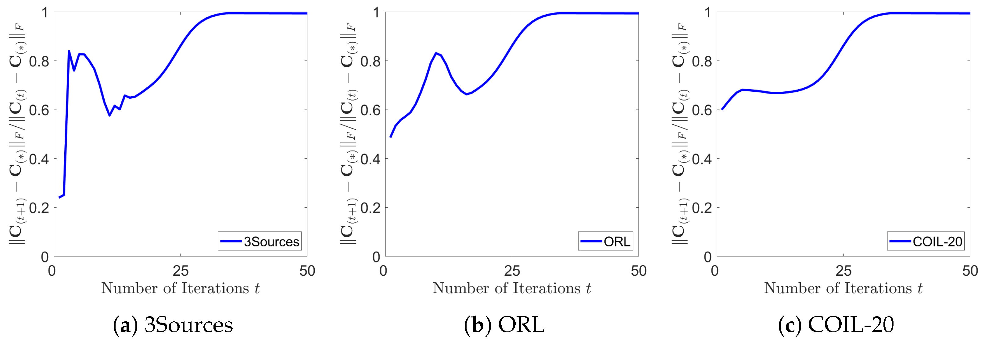
5.6. Convergence Analysis

In this convergence analysis test, we carry out experiments to provide empirical evidence of the convergence behavior exhibited by the proposed method. Through these experiments, we aim to provide robust empirical evidence that substantiates the efficiency and reliability of the method’s convergence properties. Without compromising generality, we plot the error curves of the 3Sources, ORL, and COIL-20 datasets, where the parameters are fixed at $\beta =1$, $\alpha =100$, $\gamma =0.1$, and $\sigma =9$. For ease of representation, we use $\left(t\right)$ in the subscript to denote the number of iterations. Since $\mathbf{C}$ is used for the final clustering, we focus on the convergent behavior of $\left\{{\mathbf{C}}_{\left(t\right)}\right\}$. In this test, we cancel the other termination conditions and run our algorithm for 200 iterations. Then, we plot the first 200 values of the sequence $\{\parallel {\mathbf{C}}_{(t+1)}-{\mathbf{C}}_{\left(t\right)}{\parallel }_F\}$ that are generated on the 3Sources, ORL, and COIL-20 datasets in Figure 6. Based on the experimental results, we find that the CISCAL-MVC converges in approximately 50 iterations, which is quite significant.

Next, we undertake additional experiments to delve deeper into the convergent behavior of the CISCAL-MVC. In particular, we treat ${\mathbf{C}}_{\left(200\right)}$ as the convergent solution, which is denoted as ${\mathbf{C}}_{(\ast )}$ for clarity. Then, we plot the first 50 values of the sequence $\{\parallel {\mathbf{C}}_{(t+1)}-{\mathbf{C}}_{(\ast )}{\parallel }_F/\parallel {\mathbf{C}}_{\left(t\right)}-{\mathbf{C}}_{(\ast )}{\parallel }_F\}$ that are generated on the 3Sources, ORL, and COIL-20 datasets in Figure 7, respectively. From the results, we may observe that the values of $\{\parallel {\mathbf{C}}_{(t+1)}-{\mathbf{C}}_{(\ast )}{\parallel }_F/\parallel {\mathbf{C}}_{\left(t\right)}-{\mathbf{C}}_{(\ast )}{\parallel }_F\}$ are in the range of $[0,1]$; this means that CISCAL-MVC has about a linear convergent rate.

These observations confirm the convergent behavior of the CISCAL-MVC, as well as its efficiency, that is essentially important for learning algorithms for guaranteed performance.

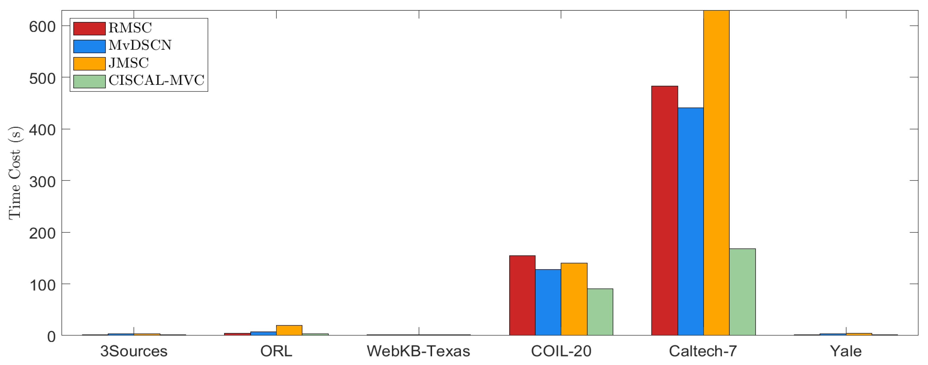
5.7. Comparison of Time Cost

In this test, we compare the time cost of our method with the baselines. Among the baseline methods, the MvDSCN and JSMC show the second and third best performance. Among the remaining baseline methods, the RMSC shows relatively better performance. Since the clustering result is essential, for clarity of presentation, we only compare our method with the above three baseline methods that show superior performance among these methods.

First, we compare the time complexity of these methods. In particular, the MvDSCN, RMSC and JSMC have time complexity of $\mathcal{O}\left(2{\sum }_{v=1}^V(n^3+2{\sum }_{l=1}^D{M}_l^2{K}_l^2{Q}_{l-v}{Q}_l)\right)$, $\mathcal{O}(V{n}^2+n^3+nk)$, $\mathcal{O}\left(V{n}^3\right)$, respectively, Where M represents the spatial dimension of the input data, l represents the l-th convolutional layer, Q represents the number of convolutional kernels in that layer, and K represents the size of each convolutional kernel. It can be seen that the non-deep learning methods generally require $\mathcal{O}\left(n^3\right)$ complexity, which are comparable. Next, we empirically compare the time cost of these methods in Figure 8. From the results, it can be seen that the CISCAL-MVC is several times faster than the RMSC and JMSC on the COIL-20 and Caltech-7 datasets. On other datasets, such as the 3Sources, WebKB-Texas, and Yale, all methods terminate within a few seconds. These observations confirm that the CISCAL-MVC is at least comparable to, if not faster than, the baseline methods from both theoretical time complexity and empirical time cost perspectives. Considering the superiority of the CISCAL-MVC in clustering performance, such time cost is acceptable.

5.8. Parametric Sensitivity

In this experiment, we empirically investigate the impact of key parameters on the learning performance of the proposed method. Without loss of generality, we use the ORL dataset to present the results in Figure 9, with fixed values of $\mu =?$ and $\kappa =?$. To systematically evaluate parameter sensitivity, we vary the parameters over the following ranges: $\alpha \in \{0.001,0.01,\dots ,1000\}$, $\beta \in \{0.001,0.01,\dots ,1000\}$, $\gamma \in \{0.001,0.01,\dots ,1000\}$, and $\sigma \in \{1,2,\dots ,10\}$. For each parameter, we analyze its individual impact on the performance of CISCAL-MVC while keeping the other parameters optimized. The experimental results reveal that the performance of CISCAL-MVC exhibits minimal variation across different values of $\alpha$ and $\sigma$, indicating robustness to these parameters. Furthermore, CISCAL-MVC achieves superior performance when smaller values are selected for $\beta$ and $\gamma$. Notably, the method demonstrates competitive performance across a wide range of small values for $\beta$ and $\gamma$ These findings suggest that CISCAL-MVC is generally insensitive to its parameter settings. For practical implementation, we recommend selecting small values for $\beta$ and $\gamma$, while adopting moderate values for $\alpha$ and $\sigma$.

5.9. Data Reconstruction

In this test, we conduct experiments to empirically showcase how the consistency and inconsistency parts of the representation capture features from the data. For illustrative purposes, and without compromising generality, we use the Yale and ORL datasets. Since the Yale dataset does not contain pixel features, we additionally introduce the original pixel features to the dataset as the 4-th view and use the augmented data $\mathbf{X}$ to learn $\mathbf{C}$ and $\mathcal{E}$, which provides a clearer visualization of the learning effects. Then, we visually show some of the original and reconstructed features in Figure 10, respectively. Based on the results, we make the following key observations: First, the features reconstructed by the overall representation matrix capture well the information from the original data, where the recovered features are visually close to the original ones. Second, the features reconstructed by the consistency part well capture the key features of the data, and the reconstructed features of different samples within the same group are visually similar with strong commonness. Third, the features captured by the inconsistency part show the diversity of the samples. These findings highlight the importance of both the consistency and inconsistency components of the representation in capturing different types of features.

6. Conclusions

In this paper, a novel approach for multi-view subspace clustering, named CISCAL-MVC, is presented. First, the novel method utilizes an adaptive loss function, which is more flexible to account for noise effects. Moreover, both the consistency and inconsistency parts of the representation matrices are exploited across different views. In particular, the consistency part exhibits hard commonness with the desired structural property, while the inconsistency part captures cross-mode sparsity to account for cross-mode differences. Then, the cross-mode sparsity constraints promote the inconsistency part to effectively exploit high-order information, thereby enhancing the consistency part to reveal high-order information of the data as well. The effectiveness and superiority of the proposed method are confirmed by extensive experiments.

Despite the effectiveness of CISCAL-MVC, there are still several aspects that could be further improved. First, the high time complexity of CISCAL-MVC limits its scalability to large-scale datasets. One potential solution to enhance efficiency is to adopt the anchor-based strategy, which approximates the representation of samples using a selected set of anchor points. This approach can be formulated as: ${\mathbf{X}}^{\left(v\right)}\approx {\mathbf{A}}^{\left(v\right)}(\tilde{\mathbf{C}}+{\tilde{\mathcal{E}}}^{\left(v\right)})$, where $\mathbf{A}\in {\mathbb{R}}^{d_v\times m}$ are the anchors, m is the number of anchor points, $\tilde{\mathbf{C}}\in {\mathbb{R}}^{m\times n}$ denotes the consistency representation, and $\tilde{\mathcal{E}}\in {\mathbb{R}}^{m\times n\times V}$ is the inconsistent part of the representation. Since $m\ll n$, the approach may significantly reduce the time complexity of the CISCAL-MVC. Second, while the current formulation of CISCAL-MVC incorporates the local geometric structure of the data on a manifold, it may not effectively capture the complex high-order neighbor relationships inherent in the data [54]. To address this limitation, inspired by recent advancements in graph-based learning [55], a high-order neighbor graph could be constructed to better preserve the intricate relationships among samples. This would allow the method to leverage more sophisticated structural information, potentially leading to improved clustering performance. Third, the proposed method requires that the dataset contains complete entries. For incomplete multi-view data, we present a potential approach as follows. We may first learn incomplete affinity matrices of the data using the observed entries. Then, we may adopt a low-rank tensor recovery technique to complete the affinity tensor for the subsequent learning procedure. However, since incomplete multi-view clustering is often considered as a different task from the general multi-view clustering [56], we do not fully expand this line of research in our current work.

The primary objective of this work is to develop a novel multi-view clustering framework that effectively utilizes cross-view high-order information, spatial structure, and both consistency and diversity across views. While the aforementioned improvements, such as anchor-based efficiency enhancement and high-order graph construction, could further advance the performance and scalability of CISCAL-MVC, they are beyond the scope of this paper. These directions, however, present promising avenues for future research.

References

1. Lei, T.; Liu, P.; Jia, X.; Zhang, X.; Meng, H.; Nandi, A.K. Automatic fuzzy clustering framework for image segmentation. IEEE Trans. Fuzzy Syst. 2019, 28, 2078–2092. [Google Scholar]
2. Peng, C.; Zhang, J.; Chen, Y.; Xing, X.; Chen, C.; Kang, Z.; Guo, L.; Cheng, Q. Preserving bilateral view structural information for subspace clustering. Knowl.-Based Syst. 2022, 258, 109915. [Google Scholar] [CrossRef]
3. Park, N.; Rossi, R.; Koh, E.; Burhanuddin, I.A.; Kim, S.; Du, F.; Ahmed, N.; Faloutsos, C. Cgc: Contrastive graph clustering forcommunity detection and tracking. In Proceedings of the ACM Web Conference 2022, Lyon, France, 25–29 April 2022; pp. 1115–1126. [Google Scholar]
4. Gönen, M.; Margolin, A.A. Localized data fusion for kernel k-means clustering with application to cancer biology. In Proceedings of the Advances in Neural Information Processing Systems, Quebec, QC, Canada, 8–13 December 2014; pp. 1305–1313. [Google Scholar]
5. Guan, R.; Zhang, H.; Liang, Y.; Giunchiglia, F.; Huang, L.; Feng, X. Deep feature-based text clustering and its explanation. IEEE Trans. Knowl. Data Eng. 2020, 34, 3669–3680. [Google Scholar]
6. Peng, C.; Kang, Z.; Li, H.; Cheng, Q. Subspace clustering using logdeterminant rank approximation. In Proceedings of the 21th ACM SIGKDD International Conference on Knowledge Discovery and Data Mining, Sydney, Australia, 10–13 August 2015; pp. 925–934. [Google Scholar]
7. Liu, G.; Lin, Z.; Yan, S.; Sun, J.; Yu, Y.; Ma, Y. Robust recovery of subspace structures by low-rank representation. IEEE Trans. Pattern Anal. Mach. Intell. 2012, 35, 171–184. [Google Scholar]
8. Peng, C.; Zhang, Y.; Chen, Y.; Kang, Z.; Chen, C.; Cheng, Q. Log-based sparse nonnegative matrix factorization for data representation. Knowl.-Based Syst. 2022, 251, 109127. [Google Scholar]
9. Vidal, R.; Ma, Y.; Sastry, S. Generalized principal component analysis (gpca). IEEE Trans. Pattern Anal. Mach. Intell. 2005, 27, 1945–1959. [Google Scholar] [CrossRef]
10. Rao, S.; Tron, R.; Vidal, R.; Ma, Y. Motion segmentation in the presence of outlying, incomplete, or corrupted trajectories. IEEE Trans. Pattern Anal. Mach. Intell. 2009, 32, 1832–1845. [Google Scholar]
11. Sun, M.; Zhang, P.; Wang, S.; Zhou, S.; Tu, W.; Liu, X.; Zhu, E.; Wang, C. Scalable multi-view subspace clustering with unified anchors. In Proceedings of the 29th ACM International Conference on Multimedia, Chengdu, China, 20–24 October 2021; pp. 3528–3536. [Google Scholar]
12. Peng, C.; Kang, Z.; Cheng, Q. Subspace clustering via variance regularized ridge regression. In Proceedings of the IEEE Conference on Computer Vision and Pattern Recognition, Honolulu, HI, USA, 21–26 July 2017; pp. 2931–2940. [Google Scholar]
13. Elhamifar, E.; Vidal, R. Sparse subspace clustering: Algorithm, theory, and applications. IEEE Trans. Pattern Anal. Mach. Intell. 2013, 35, 2765–2781. [Google Scholar]
14. Wang, F.; Chen, C.; Peng, C. Essential low-rank sample learning for group-Aware subspace clustering. IEEE Signal Process. Lett. 2023, 30, 1537–1541. [Google Scholar]
15. Zhang, C.; Fu, H.; Hu, Q.; Cao, X.; Xie, Y.; Tao, D.; Xu, D. Generalized latent multi-view subspace clustering. IEEE Trans. Pattern Anal. Mach. Intell. 2018, 42, 86–99. [Google Scholar]
16. Wang, H.; Yang, Y.; Liu, B. Gmc: Graph-based multi-view clustering. IEEE Trans. Knowl. Data Eng. 2019, 32, 1116–1129. [Google Scholar] [CrossRef]
17. Zhan, K.; Zhang, C.; Guan, J.; Wang, J. Graph learning for multiview clustering. IEEE Trans. Cybern. 2017, 48, 288–2895. [Google Scholar] [CrossRef]
18. Kumar, A.; Rai, P.; Daume, H. Co-regularized multi-view spectral clustering. In Proceedings of the Advances in Neural Information Processing Systems, Granada, Spain, 12–17 December 2011; pp. 1413–1421. [Google Scholar]
19. Wang, X.; Guo, X.; Lei, Z.; Zhang, C.; Li, S.Z. Exclusivity-consistency regularized multi-view subspace clustering. In Proceedings of the IEEE Conference on Computer Vision and Pattern Recognition, Honolulu, HI, USA, 21–26 July 2017; pp. 923–931. [Google Scholar]
20. Bai, R.; Huang, R.; Qin, Y.; Chen, Y.; Xu, Y. A structural consensus representation learning framework for multi-view clustering. Knowl.-Based Syst. 2024, 283, 111132. [Google Scholar] [CrossRef]
21. Wu, J.; Lin, Z.; Zha, H. Essential tensor learning for multi-view spectral clustering. IEEE Trans. Image Process. 2019, 28, 5910–5922. [Google Scholar] [PubMed]
22. Xia, R.; Pan, Y.; Du, L.; Yin, J. Robust multi-view spectral clustering via low-rank and sparse decomposition. In Proceedings of the AAAI Conference on Artificial Intelligence, Québec, QC, Canada, 27–31 July 2014; pp. 2149–2155. [Google Scholar]
23. Li, R.; Zhang, C.; Fu, H.; Peng, X.; Zhou, T.; Hu, Q. Reciprocal multi-layer subspace learning for multi-view clustering. In Proceedings of the IEEE/CVF International Conference on Computer Vision, Seoul, Republic of Korea, 27 October–2 November 2019; pp. 8172–8180. [Google Scholar]
24. Zhang, C.; Fu, H.; Liu, S.; Liu, G.; Cao, X. Low-rank tensor constrained multiview subspace clustering. In Proceedings of the IEEE International Conference on Computer Vision, Santiago, Chile, 7–13 December 2015; pp. 1582–1590. [Google Scholar]
25. Luo, S.; Zhang, C.; Zhang, W.; Cao, X. Consistent and specific multi-view subspace clustering. In Proceedings of the AAAI Conference on Artificial Intelligence, New Orleans, LA, USA, 2–7 February 2018; pp. 3730–3737. [Google Scholar]
26. Chen, J.; Yang, S.; Mao, H.; Fahy, C. Multiview subspace clustering using low-rank representation. IEEE Trans. Cybern. 2021, 52, 12364–12378. [Google Scholar] [CrossRef]
27. Li, D.; Wang, T.; Chen, J.; Lian, C.; Zeng, Z. Multi-view class incremental learning. Inf. Fusion 2024, 102, 102021. [Google Scholar] [CrossRef]
28. Liu, S.; Wang, S.; Zhang, P.; Xu, K.; Liu, X.; Zhang, C.; Gao, F. Efficient One-Pass Multi-View Subspace Clustering with Consensus Anchors. In Proceedings of the AAAI Conference on Artificial Intelligence, Online, 22 February–1 March 2022; pp. 7576–7584. [Google Scholar]
29. Nie, F.; Wang, H.; Huang, H.; Ding, C. Adaptive loss minimization for semisupervised elastic embedding. In Proceedings of the Twenty-Third International Joint Conference on Artificial Intelligence, Beijing, China, 3–9 August 2013; pp. 1565–1571. [Google Scholar]
30. Cai, X.; Huang, D.; Zhang, G.Y.; Wang, C.D. Seeking commonness and inconsistencies: A jointly smoothed approach to multi-view subspace clustering. Inf. Fusion. 2023, 91, 364–375. [Google Scholar]
31. Cai, D.; He, X.; Han, J. Graph regularized nonnegative matrix factorization for data representation. IEEE Trans. Pattern Anal. Mach. Intell. 2010, 33, 1548–1560. [Google Scholar]
32. Lu, C.; Feng, J.; Lin, Z.; Mei, T.; Yan, S. Subspace clustering by block diagonal representation. IEEE Trans. Pattern Anal. Mach. Intell. 2018, 41, 48–501. [Google Scholar] [CrossRef]
33. Dattorro, J. Convex Optimization & Euclidean Distance Geometry, 2nd ed.; Meboo Publishing: Palo Alto, CA, USA, 2018. [Google Scholar]
34. Bartels, R.H.; Stewart, G.W. Solution of the matrix equation AX + XB = C. Commun. ACM 1972, 15, 820–826. [Google Scholar] [CrossRef]
35. Golub, G.; Nash, S.; Van, C. A Hessenberg-Schur method for the problem AX + XB= C. IEEE Trans. Autom. Control. 1979, 24, 909–913. [Google Scholar]
36. Xie, X.; Guo, X.; Liu, G.; Wang, J. Implicit block diagonal low-rank representation. IEEE Trans. Image Process. 2017, 27, 477–489. [Google Scholar] [CrossRef] [PubMed]
37. McCoy, M.B.; Tropp, J.A. Two proposals for robust pca using semidefinite programming. Electron. J. Stat. 2010, 5, 1123–1160. [Google Scholar] [CrossRef]
38. Wang, H.; Li, H.; Fu, X. Auto-weighted mutli-view sparse reconstructive embedding. Multimed. Tools Appl. 2019, 78, 30959–30973. [Google Scholar] [CrossRef]
39. Hu, Z.; Nie, F.; Wang, R.; Li, X. Multi-view spectral clustering via integrating nonnegative embedding and spectral embedding. Inf. Fusion 2020, 55, 251–259. [Google Scholar] [CrossRef]
40. Craven, M.; DiPasquo, D.; Freitag, D.; McCallum, A.; Mitchell, T.; Nigam, K.; Slattery, S. Learning to extract symbolic knowledge from the world wide web. In Proceedings of the AAAI Conference on Artificial Intelligence, Madison, WI, USA, 26–30 July 1998; pp. 509–516. [Google Scholar]
41. Nene, S.A.; Nayar, S.K.; Murase, H. Columbia Object Image Library (Coil-20); Department of Computer Science, Columbia University: New York, NY, USA, 1996. [Google Scholar]
42. Li, F.-F.; Fergus, R.; Perona, P. Learning generative visual models from few training examples: An incremental bayesian approach tested on 101 object categories. In Proceedings of the 2004 Conference on Computer Vision and Pattern Recognition Workshop, Washington, DC, USA, 27 June–2 July 2004; p. 178. [Google Scholar]
43. Chen, M.S.; Huang, L.; Wang, C.D.; Huang, D.; Lai, J.H. Relaxed multiview clustering in latent embedding space. Inf. Fusion 2021, 68, 8–21. [Google Scholar] [CrossRef]
44. Liu, X.; Zhu, X.; Li, M.; Wang, L.; Tang, C.; Yin, J.; Shen, D.; Wang, H.; Gao, W. Late fusion incomplete multi-view clustering. IEEE Trans. Pattern Anal. Mach. Intell. 2018, 41, 2410–2423. [Google Scholar] [CrossRef]
45. Strehl, A.; Ghosh, J. Cluster ensembles—A knowledge reuse framework for combining multiple partitions. J. Mach. Learn. Res. 2002, 3, 583–617. [Google Scholar]
46. Zhang, Z.; Liu, L.; Shen, F.; Shen, H.T.; Shao, L. Binary multi-view clustering. IEEE Trans. Pattern Anal. Mach. Intell. 2018, 41, 1774–1782. [Google Scholar] [CrossRef]
47. Huang, D.; Wang, C.D.; Peng, H.; Lai, J.; Kwoh, C.K. Enhanced ensemble clustering via fast propagation of cluster-wise similarities. IEEE Trans. Syst. Man. Cybern. Syst. 2018, 51, 508–520. [Google Scholar] [CrossRef]
48. Sharma, K.; Seal, A.; Yazidi, A.; Krejcar, O. S-Divergence-Based Internal Clustering Validation Index. Int. J. Interact. Multimedia Artif. Intell. 2023, 8, 127–139. [Google Scholar]
49. Ng, A.; Jordan, M.; Weiss, Y. On spectral clustering: Analysis and an algorithm. In Proceedings of the Advances in Neural Information Processing Systems, Vancouver, BC, Canada, 3–8 December 2001; pp. 849–856. [Google Scholar]
50. Tzortzis, G.; Likas, A. Kernel-based weighted multi-view clustering. In Proceedings of the 2012 IEEE 12th international conference on data mining, Brussels, Belgium, 10–13 December 2012; pp. 675–684. [Google Scholar]
51. Li, Y.; Nie, F.; Huang, H.; Huang, J. Large-scale multi-view spectral clustering via bipartite graph. In Proceedings of the AAAI Conference on Artificial Intelligence, Austin, TX, USA, 25–30 January 2015; pp. 2750–2756. [Google Scholar]
52. Wang, S.; Liu, X.; Zhu, X.; Zhang, P.; Zhang, Y.; Gao, F.; Zhu, E. Fast parameter-free multi-view subspace clustering with consensus anchor guidance. IEEE Trans. Image Process. 2021, 31, 556–568. [Google Scholar] [CrossRef] [PubMed]
53. Zhu, P.; Yao, X.; Wang, Y.; Hui, B.; Du, D.; Hu, Q. Multiview deep subspace clustering networks. IEEE Trans. Cybern. 2024, 54, 4280–4293. [Google Scholar]
54. Peng, C.; Kang, K.; Chen, Y. Fine-grained essential tensor learning for robust multi-view spectral clustering. IEEE Trans. Image Process. 2024, 33, 3145–3160. [Google Scholar]
55. Peng, C.; Zhang, K.; Chen, Y. Cross-view diversity embedded consensus learning for multi-view clustering. In Proceedings of the the Thirty-Third International Joint Conference on Artificial Intelligence, Jeju Island, Republic of Korea, 3–9 August 2024; pp. 4788–4796. [Google Scholar]
56. Wen, J.; Zhang, Z.; Zhang, B.; Xu, Y.; Zhang, Z. A Survey on Incomplete Multiview Clustering. IEEE Trans. Cybern. 2023, 53, 1136–1149. [Google Scholar]
Figure 1. Flowdiagram illustrating graph-based and subspace clustering-based algorithms in the field of multi-view clustering. * denotes multiplication.
Electronics 14 01847 g001
Figure 2. Flow diagram of the proposed method. * denotes multiplication.
Electronics 14 01847 g002
Figure 3. Visual examples of the image datasets. From top to bottom are ten samples selected from the ORL, COIL-20, Yale, and Caltech-7 datasets, respectively.
Electronics 14 01847 g003
Figure 4. Visual illustration of the overall, consistent, and inconsistent representation matrices of different views of the ORL dataset. In particular, we show the results of the second and third views. On the diagonal of the figures, clear group structures can be observed in the consistent representation.
Electronics 14 01847 g004
Figure 5. T−SNE illustration of the distributions of the original and recovered features of the ORL dataset. In particular, we show the results of the second and third views. The features recovered by the consistent representation have a clearer cluster structure than the original features of the data with t−SNE visualization.
Electronics 14 01847 g005
Figure 6. Plot of the first 200 values of the sequence { C ( t + 1 ) C ( t ) F } generated by the CISCAL-MVC on 3Sources, ORL, and COIL-20 datasets, respectively. C ( t + 1 ) C ( t ) F represents the absolute difference of two consecutive updates, which measures the convergent behavior of the proposed algorithm. As observed, the sequences generally converge within about 50 iterations, which shows the fast convergent property of the CISCAL-MVC.
Electronics 14 01847 g006
Figure 7. Plot of the first 50 values of the sequence { C ( t + 1 ) C ( ) F / C ( t ) C ( ) F } generated by the CISCAL-MVC on the 3Sources, ORL, and COIL-20 datasets, respectively. C ( t + 1 ) C ( ) F / C ( t ) C ( ) F represents the relative difference of two consecutive updates, which measures the convergent rate of the proposed algorithm. As observed, the values are generally within (0, 1), which empirically suggests that the CISCAL-MVC has a linear convergence rate on these datasets.
Electronics 14 01847 g007
Figure 8. Time cost of different methods for comparison. These methods are selected for comparison due to their superior clustering performance as reported in Section 5.3.
Electronics 14 01847 g008
Figure 9. Performance changes of the CISCAL-MVC with respect to different values of the parameters on the ORL dataset. In particular, in each figure, the other parameters are tuned to the best. As can be seen, the CISCAL-MVC is insensitive to α and σ and achieves superior results with a broad selection of small values for γ and β .
Electronics 14 01847 g009
Figure 10. Visualization of original and reconstructed features on the Yale dataset, where we use the pixel features X ( 1 ) for illustration. As observed from the figures, the recovered features X ( 1 ) ( C + E ( 1 ) ) well capture the information from the original features. Moreover, the consistent features X ( 1 ) C well capture the key features of the data, where the features from the same cluster have high visual similarities. In contrast, the inconsistent features X ( 1 ) E ( 1 ) are sparse and capture diverse features from the data.
Electronics 14 01847 g010