Approximation of General Functions Using Stochastic Computing

Abstract

Stochastic computing (SC) is a computational paradigm that represents numbers using Bernoulli processes. It is attractive due to its low power, low hardware complexity, and excellent noise tolerance properties. An SC algorithm that approximates arbitrary functions on $[-1,1]$ using a partial sum of Chebyshev polynomials is presented. The new method displays several advantages over existing SC methods for function approximation, including the accurate modelling of complicated functions with relatively few terms, the fact that an output sample is produced for every input sample, and the extension of the domain and range to negative numbers. As a building block of the complete algorithm, an efficient method of computing the dot product of two vectors is presented, which has a broad utility beyond the application presented here.

1. Introduction

The foundational principle of stochastic computing is the representation of a number $p\in [0,1]$ as a $\mathrm{Bernoulli}\left(p\right)$ process, which is an infinite sequence of statistically independent bits where p is the probability that any given bit is ‘1’. The representation is motivated by the facts that arithmetical operations on such bit streams are typically very hardware- and power-efficient, and the represented values are highly tolerant of bit-flip errors [1,2,3,4,5,6]. Potential future applications of SC include extremely low power edge processing, sensor conditioning for embedded/wearable thin-film devices, molecular computing, and sensing/telemetry in extreme environments where errors are frequent. Even without specifying specific applications, which may be yet to be discovered, the motivation for the ability to model arbitrary mathematical functions is self-evident.

The goal is to closely approximate a real function f over some domain $\mathcal{X}\in \mathbb{R}$ using stochastic computing methods. Approximation using partial sums of basis functions ${\varphi }_n\left(x\right)$ is considered,

$$f_N\left(x\right)=\sum _{n=0}^N{a}_n{\varphi }_n\left(x\right)$$

(1)

which converges at least pointwise to f, i.e.,

$$\underset{N\to \infty }{lim}{f}_N\left(x\right)=f\left(x\right),\forall x\in \mathcal{X}.$$

(2)

The function f is then completely defined by the set of coefficients $\left\{a_n\right\}$. In Section 4, Chebyshev polynomials are employed as the basis functions of interest.

The method developed in the paper is compared to the Bernstein polynomial approach of [7,8], which is the only existing method of arbitrary function approximation using stochastic computing. Performance results show that our approach is much more accurate as a function of complexity.

In order to extend the available mathematical machinery, the ability to represent negative numbers is required. A bipolar value x can be represented using a $\mathrm{Bernoulli}\left(p\right)$ process as follows. Given a parameter $L>0$ and the constraint that $\left|x\right|\le L$, the representation may be achieved by the following linear transformation [9]:

$$T(p;L)=L(2p-1).$$

(3)

The inverse transform is

$$T^{-1}(x;L)={\displaystyle \frac{1}{2}}\left({\displaystyle \frac{x}{L}}+1\right)$$

(4)

In the remainder of the work, the shorthand notation $B_x$ is used to refer to a $\mathrm{Bernoulli}\left(T^{-1}(x;L)\right)$ process.

The paper is organised as follows. In Section 2, prior approaches to stochastic computing-based function approximation are reviewed. In Section 3, an algorithm that implements the inner product of two vectors is presented, namely the stochastic dot product (SDP). The SDP is generally useful; however, in the context of this work, it is employed as a building block of the more general function approximation design, presented in detail in Section 4. Having defined the algorithm, Section 5 is used to demonstrate the utility of the design, investigate its behaviour in various situations, and compare its performance with existing methods. Section 6 is a discussion comparing the relative merit of this work with the Bernstein polynomial approach, and Section 7 concludes the work.

2. Existing Function Approximation Methods

Before describing the architecture, some of the current approaches to the problem of function approximation using stochastic computing are briefly reviewed.

2.1. Logic Gates with Memory

Combinations of logic gates can implement various mathematical functions by manipulating the distribution of the resulting bit stream; the canonical SC example is multiplication with a single AND gate.

Introducing memory and feedback increases the range of available functions at the cost of introducing correlations into the bit stream. For example, an AND gate with an inverter at each input and the output fed into one of the inputs implements the function $(1-p)/(2-p)$. Using symbolic algebra software, one can quickly generate tables of feedback logic circuits and their associated mathematical functions, which are always ratios of polynomials [10]. Occasionally, one of these functions turns out to be useful for a particular application, e.g., the Muller-C element [11], but the range of functions is too limited to be generally applicable.

2.2. Finite State Machines

A finite state machine (FSM) can be used to implement certain functions in SC [6,12,13,14]. State transitions are controlled by the input bits (and, hence, p), while the output bit distribution is defined by the current state. The output distributions can be matched to a desired function as described in [13]. The technique is very hardware-efficient and an excellent implementation choice for certain functions such as $\mathrm{sigmoid}$. Unfortunately, however, the FSM method is not general, and it performs poorly when modelling most functions of interest.

2.3. Spectral Methods

A spectral transform interpretation of SC combinatorial logic functions is presented in [5], along with an innovative framework for designing logic circuits to implement arbitrary multi-linear equations. Similarly to FSM, the technique is very efficient but cannot model general nonlinear functions.

2.4. Bernstein Polynomials

Setting the basis function ${\varphi }_n$ to a Bernstein polynomial of degree N,

$$P_{n,N}\left(p\right)=\left({\displaystyle \genfrac{}{}{0pt}{}{N}{n}}\right)p^n{(1-p)}^{N-n}$$

(5)

for $p\in [0,1]$, true arbitrary functions can be represented in the sense of (1) and (2) [15]. An ingenious connection with SC lies in the fact that $P_{n,N}\left(p\right)$ is also the mass function in n of a $\mathrm{Binomial}(N,p)$ distribution. After summing N input bits to obtain the binomial sample n, a bit from a $\mathrm{Bernoulli}\left(a_n\right)$ process is sampled as the output. The resulting bit stream is a $\mathrm{Bernoulli}\left(f_N\left(p\right)\right)$ process [7,8].

Of all the stochastic computing-based function approximation methods discussed in Section 2, the Bernstein polynomial method described in [7,8] is the only one capable of a general function approximation. Although elegant and innovative, this method suffers from two drawbacks. The first is that function approximation using partial sums of Bernstein basis polynomials suffers from notoriously slow convergence [15]. Compared to Chebyshev basis polynomials for functions considered in Section 5, the Bernstein partial sum can require larger values of N by a factor of 100 for a similar accuracy. This is a mathematical property unrelated to the stochastic computing-based implementation. Secondly, the method described above produces only a single output bit for each N input bits. A true $\mathrm{Bernoulli}\left(p\right)$ process can be expensive, and so, ideally, an output would be generated for every input (the entropy of the input and the information-theoretic relationship between stochastic inputs and outputs is explored in [16]).

3. Stochastic Dot Product

In this section, an algorithm to compute the vector dot product $\mathbf{c}·\mathbf{x}={\sum }_{k=1}^K{c}_k{x}_k$ is described, where $\mathbf{c}$ is a length-K vector of pre-defined integers, and $\mathbf{x}$ is an arbitrary length-K vector with the constraint that $\left|x_k\right|\le L$. The constraint on $\mathbf{x}$ allows for implementation as a bipolar stochastic circuit, with output $x_o$ defined as

$$x_o=\mathrm{sign}(\mathbf{c}·\mathbf{x})min(L,\left|\mathbf{c}·\mathbf{x}\right|).$$

(6)

In other words, $x_o$ is the desired dot product saturated at $\pm L$, as imposed by the stochastic bipolar representation. Note that the integers $c_k$ are unconstrained; only $|\mathbf{c}·\mathbf{x}|\le L$ is required. A special case of the SDP is the integer scaling of a single bipolar bit stream, enabled by setting $K=1$.

We allow a deviation from classical stochastic computing techniques by introducing some deterministic operations, the most complex of which is a sum of two integers.

The SDP requires selection of an even sample period $M>1$. At each time $m\in \{1,\cdots ,M\}$ within the sample period, an output is the bit $b_{o,m}$, and an input is a set of K bits $\{b_{1,m},\cdots ,b_{K,m}\}$, with bit $b_{k,m}$ being drawn from $B_{x_k}$.

The SDP has a delay of M samples, where a set of M outputs is computed based on the previous M inputs. The SDP works for a general M; however, as will be shown in Section 3.6, the architecture benefits greatly in terms of efficiency if M is as large as possible, and also if M is selected to be a power of 2.

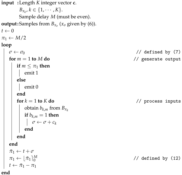
As a reference for the detailed description of each algorithm component in the remainder of the section, the complete SDP algorithm is listed in Algorithm 1.

Algorithm 1: Stochastic Dot Product Algorithm

3.1. Output Bit Stream

The output bit stream is required to be a $B_{x_o}$ process. In order to approximate the correct distribution after receiving M inputs, a $\mathrm{Bernoulli}\left({\widehat{p}}_o\right)$ distribution is imposed on the subsequent M output bits. Parameter ${\widehat{p}}_o$ is the local empirical estimate of $p_o=T^{-1}(x_o;L)$, with the constraint that ${\pi }_1={\widehat{p}}_{o}M$ is an integer. The output is given the desired distribution using one of the following options.

Option 1: Emit M samples from a $\mathrm{Bernoulli}\left({\widehat{p}}_o\right)$ distribution. For $M=2$, this rule becomes

$$b_{o,m}\leftarrow \left\{\begin{array}{cc}0,\hfill & {\pi }_1=0\hfill \\ u_m,\hfill & {\pi }_1=1\hfill \\ 1,\hfill & {\pi }_1=2\hfill \end{array}\right.$$

where $u_m$ is a sample from a uniform binary distribution.

Option 2: Emit $b_{o,m}\leftarrow 1$ for each of the first ${\pi }_1$ outputs and $b_{o,m}\leftarrow 0$ for the remaining $M-{\pi }_1$ outputs.

In this work, we exclusively used Option 2, which has a simpler implementation, being deterministic given ${\pi }_1$. The drawback of Option 2 is the introduction of correlations into the output bit sequence.

3.2. Empirical Distribution

It remains to determine ${\widehat{p}}_o$ or, equivalently, ${\pi }_1$.

At the beginning of each M-input period, initialise integer $\sigma \leftarrow {\sigma }_0$, where

$${\sigma }_0={\displaystyle \frac{M}{2}}\left(1-\sum _{k=1}^K{c}_k\right),$$

(7)

which is a constant that can be computed offline and stored at circuit creation. At each input time $m\in 1,\cdots ,M$, for each of the K inputs $b_{k,m}$, update $\sigma$ according to

$$\sigma \leftarrow \sigma +c_k{b}_{k,m},$$

(8)

i.e., increment $\sigma$ by the constant $c_k$ when the input bit corresponding to $x_k$ is 1.

After receiving M inputs, the mean $\mathrm{E}\left[\sigma \right]=p_{o}M$ is precisely the quantity of interest, namely M times the unipolar representation of the dot product (6). To verify, expand the mean as

$$\begin{array}{cc}\hfill \mathrm{E}\left[\sigma \right]& ={\sigma }_0+\mathrm{E}\left[\sum _{k=1}^K\sum _{m=1}^M{c}_k{b}_{k,m}\right]\hfill \\ \hfill & ={\displaystyle \frac{M}{2}}\left(1-\sum _{k=1}^K{c}_k\right)+M\sum _{k=1}^K{c}_k{p}_k\hfill \\ \hfill & ={\displaystyle \frac{M}{2}}\left(1+\sum _{k=1}^K{c}_k(2p_k-1)\right).\hfill \end{array}$$

(9)

The corresponding bipolar output is

$$\begin{array}{cc}\hfill x_o& =T(p_o;L)\hfill \\ \hfill & =L\left(2\left({\displaystyle \frac{\mathrm{E}\left[\sigma \right]}{M}}\right)-1\right)\hfill \\ \hfill & =\sum _{k=1}^K{c}_{k}L(2p_k-1)\hfill \\ \hfill & =\sum _{k=1}^K{c}_k{x}_k,\hfill \end{array}$$

(10)

where the substitution from (3) in the last line yields the desired result.

3.3. Bit Stream Correlations

Note that the order of summation in (8) does not affect the result, making the SDP impervious to correlations in each M-input bit sequence. In Section 4, we cascade an arbitrary number of SDPs in series; this observation allows the output bit stream of each to be assigned according to Option 2 in Section 3.1. The output of the final SDP can be assigned according to Option 1 if downstream correlations need to be avoided.

3.4. Averaging Across Sample Periods

Recall that ${\pi }_1={\widehat{p}}_{o}M$ is the local estimate of the output distribution. In practice, the circuit measures ${\overline{\pi }}_1$, which is an unconstrained estimate that may not actually be implementable unless $0\le {\overline{\pi }}_1\le M$. This unconstrained estimate ${\overline{\pi }}_1$ is computed as

$${\overline{\pi }}_1\leftarrow t+\sigma ,$$

(11)

where the integer t is defined below. Using the clamping function (defined strictly for $a<b$)

$${\lfloor i\rceil }_a^b=\left\{\begin{array}{cc}a,\hfill & i<a\hfill \\ b,\hfill & i>b\hfill \\ i,\hfill & \mathrm{otherwise},\hfill \end{array}\right.$$

(12)

an implementable value can be obtained using

$${\pi }_1\leftarrow {\lfloor {\overline{\pi }}_1\rceil }_0^M.$$

(13)

The truncated value ${\pi }_1$ is then used to generate the desired output distribution according to Section 3.1.

Finally, in order to account for the nonlinearity of the clamping function, the SDP maintains an accumulator

$$t\leftarrow {\overline{\pi }}_1-{\pi }_1$$

(14)

which is updated after each measurement of ${\pi }_1$.

The rationale for the accumulator is that if an instantaneous value of ${\overline{\pi }}_1$ cannot be represented explicitly, the “excess” value is stored until it can be represented in the output bit stream at some point in the future. Considering the ratio of total ‘1’s to total ‘0’s over many samples of ${\pi }_1$, the accumulator t ensures that the overall output distribution is correct, even if it is locally skewed by the clamping function. Each time t crosses zero, the distribution of all previous outputs in totality is just the unbiased empirical estimate of $\sigma$.

3.5. Accumulator Stability

It is instructive to consider the accumulator behaviour when $t\ll 0$. In this case, ${\pi }_1=0$ and

$$\begin{array}{cc}\hfill \mathrm{E}[{\overline{\pi }}_1-{\pi }_1]& =t+\mathrm{E}\left(\sigma \right)-{\pi }_1\hfill \\ \hfill & =t+p_{o}M\hfill \end{array}$$

and, hence, t increases over time at a rate proportional to $p_o$ while the condition remains true. Similarly, if $t\gg M$, then ${\pi }_1=M$ and

$$\mathrm{E}[{\overline{\pi }}_1-{\pi }_1]=t-(1-p_o)M,$$

which decreases over time. This negative feedback ensures that the value of t will always eventually return to zero.

While the accumulator is stable in expectation, the zeroing effect is relatively slow and the accumulator is prone to large local perturbations if the variance of $\sigma$ is significantly greater than M. The effect on t of a large sample $\sigma =s$ where $s\gg M$ will take a minimum of $s/M$ sample periods to remove, during which time the output bit stream will be all ‘1’s.

The variance can be quantified as

$$\begin{array}{cc}\hfill \mathrm{Var}\left[\sigma \right]& =\mathrm{Var}\left[\sum _{k=1}^K\sum _{m=1}^M{c}_k{b}_{k,m}\right]\hfill \\ \hfill & =\sum _{k=1}^K{c}_k^2\sum _{m=1}^M\mathrm{Var}\left[b_{k,m}\right]\hfill \\ \hfill & =M\sum _{k=1}^K{c}_k^2{p}_k(1-p_k),\hfill \end{array}$$

(15)

which is maximized when the values of $p_k$ are all equal to $1/2$ (equivalently $x_k=0)$. Assuming the values of $p_k$ are uniformly distributed, their influence can be averaged out to obtain

$$\begin{array}{cc}\hfill {\mathrm{E}}_p\left[\mathrm{Var}\left[\sigma \right]\right]& ={\int }_0^{1}M\sum _{k=1}^K{c}_k^{2}p(1-p)dp\hfill \\ \hfill & ={\displaystyle \frac{M}{6}}\sum _{k=1}^K{c}_k^2.\hfill \end{array}$$

(16)

The above expression demonstrates that when algorithms are designed with the SDP as a building block, the magnitude of constants $c_k$ critically affects the stability of the circuit.

3.6. SDP Complexity

If an SC architecture such as the SDP finds widespread practical utility, it will likely be associated with a newer and more novel technology than classical CMOS. Rather than introducing various assumptions required to compute die area and gate counts, the complexity discussion will remain as general as possible.

In the main algorithm implementation presented in Section 4, the elements of vector $\mathbf{c}$ are small constant integers ($|c_k|\le 2$), and as such the increment (8) has an efficient hardware implementation.

If M is chosen as a power of 2, Equation (14) is trivial when ${\overline{\pi }}_1\le M$ and, otherwise, is performed by simply flipping bits from bit $\mu$ towards the most-significant bit (MSB) until a ‘1’ is found (where $\mu =1+{log}_{2}M$). Similarly, the function (13) has a very simple implementation.

The bulk of the hardware complexity resides in the general addition (11), which is performed once every M input samples. Notwithstanding the discussion in Section 3.4 regarding the accumulator behaviour, the magnitude of t (and, hence, the size of the register required to contain ${\overline{\pi }}_1$) is theoretically unbounded. For the simulations in Section 5, 16 bits was more than enough to safely represent ${\overline{\pi }}_1$, and further optimization is likely possible.

Finally, given that the operations discussed here are only performed once every M bits, it is prudent to consider using larger values of M. Experiments showed that M could be varied between 2 and 1024 without affecting the accuracy or precision.

3.7. Alternative Dot-Product Methods

While the SDP was developed specifically for the application described in Section 4, other dot-product approaches, or techniques that could be applied to such, have been described in the literature [12,14,17,18,19,20,21]. These were not considered here for the following reasons.

• In our application, one of the dot product inputs is a vector of integers, which is known at circuit creation. We wish to exploit this fact in order to reduce noise.
• It is unclear how to adapt existing methods to represent unconstrained integer inputs, or to produce a bipolar output $\left|x\right|\le L$.

On the other hand, a drawback of the proposed SDP is the use of deterministic binary additions. An attempt to adapt existing dot-product methods to this application in order to eliminate additions would be a worthwhile future endeavour.

4. Chebyshev Function Approximation

The goal is to approximate an arbitrary function $f\left(x\right)$ on $[-1,1]$ as the partial sum

$$f_N\left(x\right)=\sum _{n=0}^N{a}_n{T}_n\left(x\right)$$

(17)

where $T_n\left(x\right)=cos\left(n{cos}^{-1}\left(x\right)\right)$ is the nth Chebyshev polynomial of the first kind [22,23]. Chebyshev polynomials are an excellent basis for function approximation due to their simplicity and low error for a given N, and as such, they are frequently applied in numerical computing applications [24,25]. The computation of the coefficients $a_n$ was performed offline and is not considered here [26].

Since $T_n\left(x\right)$ can be expressed as a degree-n polynomial in x with integer coefficients, in principle, it could be computed directly using the SDP along with a circuit that raises x to an integer power (a sequence of n XNOR gates in series implements $x^n/L^{n-1}$). Unfortunately, the coefficients of $T_n\left(x\right)$ increase rapidly in magnitude with n, leading to large accumulator excursions in the SDP implementation. To illustrate, the variance (16) for the SDP implementation of $T_{13}\left(x\right)$ is approximately ${10}^{8}M$.

4.1. Stochastic Clenshaw Algorithm

To obtain a more stable and efficient implementation, the Clenshaw algorithm [27] can be applied to compute (17). Stating the algorithm directly, the partial sum can be expressed as

$$f_N\left(x\right)=a_0+x{g}_1\left(x\right)-g_2\left(x\right)$$

(18)

where the $g_n\left(x\right)$ are defined by the recurrence relation

$$g_n\left(x\right)=a_n+2x{g}_{n+1}\left(x\right)-g_{n+2}\left(x\right),$$

(19)

initialised by

$$g_{N+1}\left(x\right)=g_{N+2}\left(x\right)=0.$$

(20)

The algorithm suggests a direct stochastic implementation as $N+1$ cascaded repeating circuit stages, with each circuit implementing one stage of the recurrence (19).

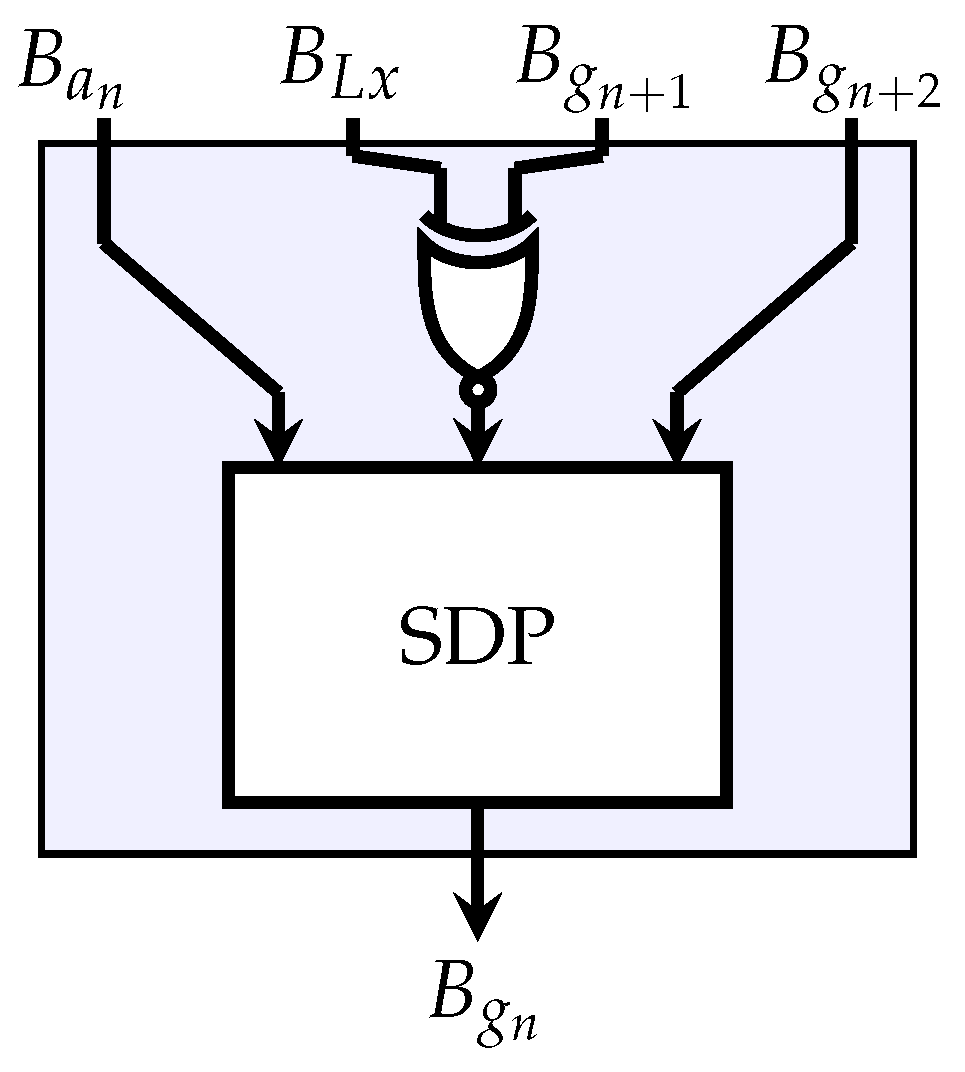
4.1.1. Clenshaw Stage

Equation (19) can expressed as the dot product of vectors $\mathbf{x}=[a_n,x{g}_{n+1},g_{n+2}]$ and $\mathbf{c}=[1,2,-1]$, which immediately suggests the use of an SDP. The stochastic representation of the product $x{g}_{n+1}$ can be computed with an XNOR gate on the output of $B_x$ and $B_{g_{n+1}}$, which yields the bipolar representation of $x{g}_{n+1}/L$ [9,28]. The combined circuit representing one stage of the stochastic Clenshaw algorithm is shown in Figure 1.

In order to account for the $1/L$ scale factor introduced by the XNOR gate, the corresponding SDP constant could be scaled as $\mathbf{c}=[1,2L,-1]$ (assuming $2L$ is an integer). Given the expression for variance (16), however, and the fact that many such stages will be cascaded, scaling the constant in this way significantly increases the noise level. Since x is only defined within $[-1,1]$, a better solution is to scale the input by L. This could be performed as part of generating the input Bernoulli process or online via a single-term SDP with $\mathbf{c}=\left[L\right]$.

4.1.2. Complete Clenshaw Circuit

Having defined a single stage, the entire algorithm can be implemented using $N+1$ stages in series, connected as shown in Figure 2. This is a direct implementation of Equations (18)–(20).

Noting the edge cases in the algorithm definition, the constant vector ${\mathbf{c}}_n$ for the SDP in stage n is defined as follows:

$${\mathbf{c}}_n=\left\{\begin{array}{cc}[1,0,0],\hfill & \mathrm{if}n=N\hfill \\ [1,2,0],\hfill & \mathrm{if}n=N-1\hfill \\ [1,1,-1],\hfill & \mathrm{if}n=0\hfill \\ [1,2,-1],\hfill & \mathrm{otherwise},\hfill \end{array}\right.$$

(21)

so the output of stage $n=0$ is the desired partial sum (17).

Once an $N+1$-stage dedicated circuit implementing Figure 2 is created, it can model any function f with an order-N partial sum simply by providing the appropriate input processes $B_{a_n}$.

One useful optimization is that in the case $a_n=0$, the process $B_{a_n}$ can be ignored, or equivalently the integer ${\left({\mathbf{c}}_n\right)}_1$ can be set to zero. This is useful to reduce the variance (16) when modelling odd or even functions, in which case $a_n=0$ for every other n.

Parallel implementations of the Clenshaw algorithm are known [29]; however, in this application, the serial implementation can be fully pipelined with no loss of throughput. Each unbiased output sample from the algorithm requires only a single sample from $B_{Lx}$, along with a single sample from each of the $B_{a_n}$.

5. Numerical Investigation

For each of the experimental results presented in this section, $S={10}^6$ input bits were presented to the stochastic circuit in order to obtain the measurement at the output. The output estimator measures $T(\sum b_o/S)$, which can be implemented using techniques in, e.g., [18]. The variance of this estimator scales as $1/S$. While $S={10}^6$ is almost certainly impractically large in real applications, for the purposes of Section 5, we seek to investigate systematic errors and biases which might otherwise be obscured by sampling noise if a smaller S were used.

Axis labels are omitted from plots in order to preserve page space; the horizontal axis always represents the independent variable x, and the vertical axis represents $f\left(x\right)$.

5.1. Examples

Some selected examples of simple modelled functions are shown in Figure 3 along with the stochastic circuit simulation results. The function definitions are listed in the caption along with the number of terms N in the partial sum.

In Figure 3a,b is shown the degree-3 polynomials in the examples from [13] and [7], respectively, extended into the bipolar domain. Since any degree-d polynomial can always be represented exactly as the sum (17) with $N=d$ [22], only four stochastic Clenshaw stages are required in each case.

Figure 3c shows a tanh function modelled with 12 Clenshaw stages. This is the curve from Example 3 of [12], shifted and scaled to be centred in the bipolar regime. In this case, the partial sum is not an exact representation but a truncated infinite sum. This represents an alternative implementation of an activation function for artificial neural networks, given recent interest in using SC for such applications [30,31].

The final subplot of Figure 3 shows the sum of two Chebyshev polynomials. This is an exact representation with only two non-zero terms appearing in (17).

Further examples are presented in Figure 4, this time for general functions with no limitation on complexity. Figure 4a,b show selected oscillatory functions with 21 terms. These are examples of transcendental functions that are complicated to implement using traditional logic.

Figure 4c shows a $\mathrm{sign}$ function modelled with $N=50$. The Gibbs phenomenon can be seen causing oscillations due to the nonlinearity at the step. Even with 51 stochastic Clenshaw stages configured in series, however, the stochastic circuit faithfully models the partial sum with low noise.

Finally, Figure 4d shows an extreme example where the method fails. The Gamma function is modelled with 61 terms over a domain containing multiple singularities and discontinuities. The right-hand side of the plot shows a somewhat accurate approximation (albeit with some oscillation), but in the left-hand side of the plot, the approximation completely breaks down due to noise propagation through the Clenshaw stages.

5.2. Choosing the Scale Parameter

The setting of parameter L in the bipolar representation (3) is a design decision to be addressed. The representation is limited to $\left|x\right|\le L$, so L should be at least as large as the expected largest value, including any intermediate values within the Clenshaw stages. If L is much larger than necessary, however, the domain of interest is mapped via (4) onto only a portion of the available unipolar space. For example, if x is in $[-1,1]$ and $L=10$, the inverse map (4) restricts p to the interval $[0.45,0.55]$, ignoring 90% of the available range of values. The experiment shown in Figure 5 explores this effect.

In the top left sub-figure, the scale is set to $L=1$. The noise appears quite small; however, the stochastic circuit is completely unable to represent $f\left(x\right)$ for $x>0.7$. The reason is that intermediate values within the Clenshaw stages violate the condition $|g_n| \le L$. These intermediate values are clipped before propagating through the circuit, and as a result, the final value of $f\left(x\right)$ is inaccurate.

In contrast, when $L=8$ (shown in the bottom right sub-figure), the output shows no evidence of clipping, but the high level of noise produces a poor approximation.

In general, for optimal performance, L should be set as small as possible, but large enough that any clipping is avoided. The appropriate value of L can be quickly investigated offline using a floating-point version of the Clenshaw algorithm as the maximum absolute intermediate value recorded. For the function shown in Figure 5, the optimal value of L is evidently between 2 and 4.

5.3. Comparison with Bernstein Approximation

Of the various function approximation methods introduced in Section 2, only the Bernstein approximation [7,8] is capable of representing general functions.

Figure 6 shows the measured squared error between a given function and the two universal approximators, as a function of the number of stages N. The squared error is averaged over 200 values of x, evenly spaced across the domain of interest. The very long sequences of input bits ($S={10}^6$) minimises sampling noise and allows for an investigation of the inherent error for each design.

In Figure 6a, the function modelled in Figure 4b is reinvestigated. As shown in Figure 4, the Chebyshev approximation gives a good fit with $N=20$ terms, corresponding to a mean squared error of roughly ${10}^{-4}$ in Figure 6a. In contrast, even with $N=200$ stages, the Bernstein approximation cannot reach this level of accuracy.

In Figure 6b, a much more complicated function is modelled, as specified in the figure caption. The Chebyshev approximator requires around $N=50$ stages to achieve a good fit. In contrast, the Bernstein approximator requires $N=1000$ to even approach this level of accuracy.

The examples discussed above were not cherry-picked; the relative difference in the required number of stages seems consistent for all functions of interest.

Interestingly, for very small values of N, the Bernstein architecture outperforms the proposed method in terms of accuracy, as can be seen in Figure 6. For such small values of N, however, the approximation remains very poor for both architectures.

6. Discussion

The examples in Section 5 clearly demonstrate the utility and performance of the proposed function approximation circuit. Some of the limitations and drawbacks are in turn discussed here.

The most notable drawback is the complexity of the $N+1$ SDPs. The deterministic operations discussed in Section 3.6 are performed $(N+1)/M$ times per output bit, the most significant of which is a signed integer addition. Noting from Section 5 that the most complicated functions can require $N\approx 50$, and setting $M=1024$, the signed addition is required around once every 20 output bits in the worst case.

Another source of complexity is the $N+1$ Bernoulli source processes representing the coefficients $a_0,\cdots ,a_N$. Whether consumed from some high-entropy source or pseudo-randomly produced within the circuit itself, the Bernoulli processes represent significant resources. The Chebyshev circuit is not unique in this regard; the Bernstein circuit also requires $N+1$ such processes representing the coefficients, and in that case, N can be at least an order of magnitude larger as observed in Section 5.3.

In the following, we refer to the circuit proposed in this work as “Chebyshev” and the circuit proposed in [7] as “Bernstein”. It is not possible to definitively rank the two circuit designs without considering the application, the technology used to implement the circuit, and the design constraints.

If the application is rate-limited, where the maximum number of output samples is required in a given time as much as possible, Chebyshev is clearly the best.

In a power-limited scenario where the source processes must be generated or conditioned in some way, Chebyshev likely consumes less power due to the greatly reduced number of Bernoulli processes representing coefficients. This will be offset somewhat by the relatively expensive processing required by Chebychev every $(N+1)/M$ inputs.

If the goal is to minimise the circuit size, the answer, again, depends on the availability of the source processes and is similarly murky. The $N+1$ SDPs used to implement Chebyshev obviously requires more logic gates than the simple 1-bit adders composing Bernstein. However, the smallest overall circuit depends on the relative size of the source processes and the fact that Bernstein requires so many more of them.

In requiring some deterministic addition operations, both approximations lose some of the tolerance to bit-flip errors characteristic of stochastic computing. For example, an error in the MSB of the integer $\sigma$ in one of the SDPs would be far more damaging to accuracy than an error in one of the input bits. If the circuit were to be used in an environment or application where bit-flip errors are common, the deterministic portions of the circuit may require additional protection of some kind.

7. Conclusions

In this work, a new stochastic computing architecture for function approximation is proposed based on a partial sum Chebyshev expansion. The method can model arbitrarily complicated functions on $[-1,1]$ with high accuracy using relatively few terms in the partial sum. Unlike other proposals in the literature, the method extends the domain over the negative numbers and has an adjustable range. The architecture is full-rate, in that an output sample is produced for every input sample.

As a core building block of the new architecture, a stochastic circuit is presented that computes the dot product of a bipolar vector with an arbitrary constant integer vector. This dot-product core has useful applications in and of itself.