Article

Estimating Calibrated Risks Using Focal Loss and Gradient-Boosted Trees for Clinical Risk Prediction

1
Department of Industrial, Manufacturing, and Systems Engineering, Texas Tech University, Lubbock, TX 79409, USA
2
Heart and Vascular Institute, Pennsylvania State University College of Medicine, Hershey, PA 17033, USA
*
Author to whom correspondence should be addressed.
Electronics 2025, 14(9), 1838; https://doi.org/10.3390/electronics14091838
Submission received: 4 February 2025 / Revised: 22 April 2025 / Accepted: 26 April 2025 / Published: 30 April 2025
(This article belongs to the Special Issue Data-Centric Artificial Intelligence: New Methods for Data Processing)

Abstract

:
Probability calibration and decision threshold selection are fundamental aspects of risk prediction and classification, respectively. A strictly proper loss function is used in clinical risk prediction applications to encourage a model to predict calibrated class-posterior probabilities or risks. Recent studies have shown that training with focal loss can improve the discriminatory power of gradient-boosted decision trees (GBDT) for classification tasks with an imbalanced or skewed class distribution. However, the focal loss function is not a strictly proper loss function. Therefore, the output of GBDT trained using focal loss is not an accurate estimate of the true class-posterior probability. This study aims to address the issue of poor calibration of GBDT trained using focal loss in the context of clinical risk prediction applications. The methodology utilizes a closed-form transformation of the confidence scores of GBDT trained with focal loss to estimate calibrated risks. The closed-form transformation relates the focal loss minimizer and the true-class posterior probability. Algorithms based on Bayesian hyperparameter optimization are provided to choose the focal loss parameter that optimizes discriminatory power and calibration, as measured by the Brier score metric. We assess how the calibration of the confidence scores affects the selection of a decision threshold to optimize the balanced accuracy, defined as the arithmetic mean of sensitivity and specificity. The effectiveness of the proposed strategy was evaluated using lung transplant data extracted from the Scientific Registry of Transplant Recipients (SRTR) for predicting post-transplant cancer. The proposed strategy was also evaluated using data from the Behavioral Risk Factor Surveillance System (BRFSS) for predicting diabetes status. Probability calibration plots, calibration slope and intercept, and the Brier score show that the approach improves calibration while maintaining the same discriminatory power according to the area under the receiver operating characteristics curve (AUROC) and the H-measure. The calibrated focal-aware XGBoost achieved an AUROC, Brier score, and calibration slope of 0.700, 0.128, and 0.968 for predicting the 10-year cancer risk, respectively. The miscalibrated focal-aware XGBoost achieved equal AUROC but a worse Brier score and calibration slope (0.140 and 1.579). The proposed method compared favorably to the standard XGBoost trained using cross-entropy loss (AUROC of 0.755 versus 0.736 in predicting the 1-year risk of cancer). Comparable performance was observed with other risk prediction models in the diabetes prediction task.

1. Introduction

Risk prediction is one of the most important tasks in clinical research. It consists of estimating the probability that an individual will experience an event or outcome of interest. A model estimates the probability of the event based on features such as age, sex, body mass index, blood type, or previous history of malignancy. Estimated probabilities are useful to group patients into different risk strata such as low or high risk. Patients in the high-risk group can receive preemptive treatment. For example, solid organ transplant recipients may be closely monitored if they are at risk of post-transplant malignancy [1]. They may also receive anti-viral medications to prevent serious adverse events arising from viral infections [2]. A solid organ donor can be matched to a specific recipient on the waiting list to improve survival after transplantation [3]. Another example of clinical risk prediction applications includes heart failure assessment. Individuals with genetic risk factors can undergo non-invasive imaging to check for heart disease [4]. Individuals at high risk for heart failure can be treated preemptively with medications to manage blood pressure [5]. Preemptive treatment can reduce heart failure diagnoses and save money for the healthcare system [6].
Risk prediction models are assessed by their discrimination or their ability to separate high-risk patients from low-risk patients. A model with perfect discriminatory power assigns higher probabilities to all patients with a medical condition or “event” and lower probabilities to patients who do not have the condition or event. The area under the receiver operating characteristics curve (AUROC) and the H-measure are evaluation metrics used to assess the discriminatory power of risk prediction models and probabilistic classifiers [7]. Clinical risk prediction models are also expected to be calibrated [8]. Estimated probabilities or risks are calibrated if they match the frequency of the event. For example, if a model provides an estimated probability of 20 % given a set of patient variables (features), then 20 out of 100 similar patients should experience the event. The evaluation of probability calibration has generally received less attention than discriminatory power, although it is important for clinical decision-making [9,10]. A miscalibrated model can underestimate or overestimate risks. Underestimation may prevent patients from receiving the necessary medical treatment, while overestimation can lead to unnecessary and costly treatment. Calibration curves, calibration slope, and intercept are commonly used in the risk prediction literature to assess probability calibration [8,10]. The Brier score metric summarizes both discrimination and calibration and is considered an overall accuracy metric [9].
One of the most commonly used models in clinical risk prediction applications is logistic regression. The logistic regression model assumes the logit (logarithmic odds) of the estimated posterior probability to be a linear function of the variables or features. Logistic regression offers a straightforward interpretation for clinical professionals. More complex machine learning models, such as gradient-boosted decision trees (GBDT), have attracted attention in medical fields, where large electronic health records are commonly used. GBDT is an iterative method that adds individual decision trees to improve the performance of an ensemble of trees [11]. GBDT has attributes that make it capable of handling electronic health records effectively. GBDT can handle heterogeneous features (numerical and categorical) available in electronic health records and identify non-linear interactions automatically. GBDT variants also offer regularization techniques to prevent overfitting noisy electronic health records [12]. Efficient implementations of GBDT include extreme gradient-boosting machine (XGBoost) [13], light gradient-boosting machine (LightGBM) [14], CatBoost [15], and PaloBoost [12].
GBDT models offer the flexibility to optimize a smooth and differentiable loss function to guide the decision tree training process. Each decision tree in the ensemble is fitted to the pseudo-residuals or negative gradient of the loss function. The standard loss function for probability estimation and classification in GBDT is the cross-entropy loss function (also known as log loss or negative log likelihood). Recent studies related to class-imbalanced data classification have combined GBDT with the focal loss function to improve classification performance [16,17,18,19,20,21,22,23]. The focal loss adds a modulating factor to the cross-entropy loss function. This factor modulates the relative loss of the samples according to the accuracy of the estimated confidence scores [24]. This modulation effect guides the training process to focus on the samples with large losses (“hard-to-classify” samples). This effect may be desirable in applications such as clinical risk prediction and object detection because it allows the training process to focus on rare and difficult samples [25,26]. Previous studies that combined GBDT with focal loss were primarily concerned with classification tasks and evaluated predictive performance based on discrimination and classification metrics. Training GBDT with focal loss leads to miscalibrated confidence scores because the loss function is not strictly proper [27]. Hence, these confidence scores cannot be interpreted as reliable class-posterior probabilities. In class probability estimation, the expected loss of a strictly proper loss function is minimized if and only if the estimated conditional distribution of the outcome variable is equal to the true distribution [28]. Therefore, strictly proper loss functions are fundamental for prediction tasks that require accurate probabilities.
In this study, we investigate the focal loss function and GBDT in the context of risk prediction and classification of clinical data with a binary label or event. A recent theoretical study on focal loss for class-posterior probability estimation proposed a closed-form transformation of confidence scores to recover the true class-posterior probabilities [27]. The transformation is known as the Ψ γ transformation. The Ψ γ transformation relates the focal loss minimizer and the true class-posterior probability. It can be applied to binary and multi-class prediction tasks that require calibrated class-posterior probabilities.
The contributions of this study are the following: (1) We investigate the application of the Ψ γ transformation to GBDT trained using focal loss and evaluate the calibration of confidence scores for clinical risk prediction. (2) We propose two algorithms based on Bayesian hyperparameter optimization and K-fold cross-validation to choose the focal loss parameter and optimize discriminatory power and calibration (as measured by the Brier score). (3) We investigate the adjustment of the decision threshold in combination with GBDT, focal loss, and Ψ γ transformation. We specifically choose a decision threshold to optimize the arithmetic mean of sensitivity and specificity (balanced accuracy) for classification. (4) We investigate the performance of these techniques in two important clinical risk prediction tasks: prediction of cancer in lung transplant recipients and prediction of diabetes. We use real datasets extracted from the Scientific Registry of Transplant Recipients (SRTR) and the Behavioral Risk Factor Surveillance System (BRFSS). We provide comparisons with GBDT trained using the standard cross-entropy loss and unregularized and regularized logistic regression. We also provide comparisons with GBDT calibrated with Platt scaling and isotonic regression.
The paper is organized as follows: Section 2 discusses previous studies on GBDT for clinical risk prediction, custom loss functions for GBDT, and probability calibration. We describe gaps in previous studies that modified the loss function of GBDT. Section 3 describes the methodology. It is divided into five subsections. Section 3.1 introduces the cross-entropy loss, focal loss, strictly proper losses, and the Ψ γ transformation for risk prediction tasks. Section 3.2 introduces the training objective of GBDT and regularized GBDT. Section 3.3 introduces Bayesian hyperparameter optimization. This section describes two algorithms to tune the GBDT and choose the focal loss parameter. We also provide a detailed discussion of hyperparameter values and distributions. Section 3.4 discusses the decision threshold that will be used to calculate the classification metrics. The section also discusses the importance of calibrated probabilities in optimizing the balanced accuracy metric for classification tasks. Section 3.5 introduces the relevant metrics for risk prediction and classification, including discrimination, calibration, and classification metrics. Section 4 describes the experiments. It is divided into three subsections. Section 4.1 describes the datasets from the SRTR and BRFSS databases. Section 4.2 describes the design of the experiments. Section 4.3 presents the results of the experiments. Section 5 provides a discussion of the study and the main results. Finally, the conclusion summarizes the study and suggests future directions for researchers.

2. Related Works

2.1. GBDT in Clinical Risk Prediction

Seto et al. studied the probability calibration of LightGBM for the prediction of diabetes using the Kokuho database from Japan. The authors reported that LightGBM produced more accurate probabilistic predictions (measured by the expected calibration error) compared to logistic regression as the sample size increased beyond 10 4  [29]. Ma et al. applied task-wise split gradient boosting trees (TSGB) to predict venous thromboembolism (VTE) across different hospital departments [30]. TSGB is based on GBDT and showed a superior discriminatory power (measured by the AUROC) compared to logistic regression. However, the study did not assess the calibration of the proposed TSGB model. Another study found XGBoost to achieve the best performance among various models in predicting graft survival after kidney transplantation [31]. The study used discrimination and classification metrics including AUROC, accuracy, sensitivity, specificity, and F1-measure, but did not assess the calibration of the model. However, other studies have found that GBDT and logistic regression have comparable performance in some clinical risk prediction tasks [32,33]. Bae et al. compared logistic regression and XGBoost in predicting kidney transplant outcomes using the Scientific Registry of Transplant Recipients (SRTR). They found that AUROC and overall accuracy (measured by the Brier score) were comparable in different tasks, such as predicting delayed graft function and acute rejection [34]. The authors found that the AUROC of the models was in the range 0.717–0.723 for the prediction of the delayed graft function. Austin et al. performed simulations using two large cardiovascular datasets to compare machine learning and statistical models [35]. They found that conventional logistic regression and GBDT had superior performance across a variety of data-generating processes. The authors used metrics such as AUROC, Brier score, calibration slope, and intercept. Miller et al. compared machine learning and statistical models and concluded that performance depended on the type of cross-validation used [36]. The authors used data from the United Network for Organ Sharing (UNOS) to predict mortality after heart transplantation. XGBoost obtained better AUROC than logistic regression in shuffled cross-validation (0.820 vs. 0.661). However, the AUROC values decreased to 0.657 and 0.641 for XGBoost and ridge logistic regression in rolling cross-validation, respectively. These studies used GBDT trained with the standard cross-entropy loss function and did not consider other loss functions such as focal loss.

2.2. GBDT and Custom Loss Functions

GBDT can handle the optimization of custom smooth loss functions. Several studies have combined GBDT with focal loss and other loss functions to mainly address problems in classifying data with imbalanced or skewed class distribution. Wang et al. compared XGBoost trained with different loss functions such as cross-entropy loss, weighted cross-entropy loss, and focal loss in Parkinson’s disease classification [16]. They reported that XGBoost combined with focal loss performed better than standard XGBoost according to the F1-score metric. Liu et al. combined a cost-sensitive version of LightGBM with focal loss to classify imbalanced credit scoring datasets [18]. The authors found that the combination of cost-sensitive learning and focal loss was superior or competitive on four different credit scoring tasks. Boldini et al. compared weighted cross-entropy loss, focal loss, logit-adjusted loss, label-distribution-aware margin loss, and equalization loss to train LightGBM for imbalanced bioassay classification [17]. The authors reported logit-adjusted loss and label-distribution-aware margin loss to achieve the most promising results in different experiments. Label-distribution-aware margin loss and logit-adjusted loss are designed to optimize classification metrics appropriate for class-imbalanced data. Cao et al. proposed the label-distribution-aware margin loss function to optimize a balanced generalization error bound [37]. Logit-adjusted loss was originally proposed as a loss function to minimize balanced error in deep long-tail learning [38]. Mushava et al. proposed unified focal loss combined with flexible link functions such as generalized extreme value (GEV) and exponentiated-exponential logistic (EEL) distribution-based link functions [19,20]. The authors used their proposed loss function to train XGBoost using the Freddie Mac mortgage loan database. They reported improvements in discriminatory power according to the H-measure metric. Rao et al. combined cost-sensitive CatBoost with focal loss for imbalanced customer churn prediction. The authors also used a modified adaptive synthetic (ADASYN) resampling approach to handle class-imbalanced data [22]. Luo et al. compared different loss functions to train LightGBM and XGBoost [23]. The authors compared weighted cross-entropy loss, focal loss, and asymmetric losses for binary, multi-class, and multi-label imbalanced datasets. They reported improvements in F1-score when training XGBoost with weighted cross-entropy and asymmetric losses. Fan et al. proposed to combine XGBoost with triage loss to diagnose vibration sensor failure [39]. The triage loss is a modification of the focal loss that further increases the weight of the hard-to-classify samples during the training process. The authors reported that XGBoost combined with triage loss outperformed XGBoost trained with cross-entropy and focal losses.
The previous studies that combined GBDT with custom losses were primarily concerned with classification tasks, so they did not assess the calibration of predicted probabilities or discuss whether the loss functions were strictly proper.

2.3. Probability Calibration

Probability calibration is concerned with the agreement between the estimated probabilities and the observed fraction of positive events. The assessment of probability calibration generally receives less attention than the assessment of discriminatory power and classification accuracy [10]. The topic has gained popularity in recent years in the literature on deep learning [40]. Studies in the area have focused on the properties of loss functions that encourage calibration, heuristics, and appropriate methods and metrics to evaluate performance. The properties of loss functions that encourage accurate probability estimation have been studied in [25,28,41,42,43,44]. Loss functions that encourage accurate probability estimation are known as strictly proper loss functions. Strictly proper loss functions are globally minimized if and only if the estimated class-posterior probabilities are equal to the ground-truth probabilities. Examples of these loss functions are the cross-entropy loss and the Brier score loss. However, note that minimization of strictly proper loss functions encourages calibration but is not sufficient to guarantee good calibration [44]. Strictly proper loss functions are also used in heuristic techniques for post hoc probability calibration. An example of a heuristic technique is the Platt scaling method proposed in [45]. In Platt scaling, a sigmoid function is applied to the predictions of a miscalibrated model. The parameters of the sigmoid function are found by minimizing the strictly proper cross-entropy loss over a calibration set or by performing a K-fold cross-validation over the training set. Temperature scaling is a variant of Platt scaling that uses a single parameter [40,46]. Temperature scaling is effective in improving the calibration of deep neural networks. Another method of calibrating probabilities is isotonic regression [47]. The isotonic regression method finds a step-wise non-decreasing function to map the miscalibrated confidence scores to calibrated probabilities. Isotonic regression can perform poorly when the sample size is small. Beta calibration is a technique that calibrates confidence scores using calibration maps based on the beta distribution [48]. Continuous model update strategies have also been studied to maintain calibration after deployment in a clinical setting [10]. Continuous update strategies are useful when the distribution of the population changes over time [49]. Many recent studies on probability calibration are also related to evaluation methods such as reliability diagrams and appropriate metrics for risk prediction applications [8,50,51].

3. Methods

This section describes the machine learning methodology for the prediction of clinical risk and the classification of data with an imbalanced or skewed class distribution. It consists of GBDT trained using focal loss, calibration, and Bayesian optimization. The proposed approach is also combined with an empirical decision threshold to optimize the arithmetic mean of sensitivity and specificity (balanced accuracy). We consider the problem of risk prediction using data with a binary class label. We also consider the classification of binary class-imbalanced data through decision threshold adjustment. Let D = { ( x i , y i ) } i = 1 n be a training set consisting of n samples, where x i X is the p-dimensional feature vector and y i { 0 , 1 } is the binary class label. The first goal is to learn a risk prediction model, q : X [ 0 , 1 ] . The risk prediction model must provide a reliable estimate of the true class-posterior probability η ( x ) = p ( y = 1 | x ) . The second goal is to learn a binary classification model δ ^ : X { 0 , 1 } , where δ ^ is an approximation of the true function δ : X { 0 , 1 } . We assign a sample to one of two classes by thresholding the class-posterior probability using a decision threshold estimated from the training data.

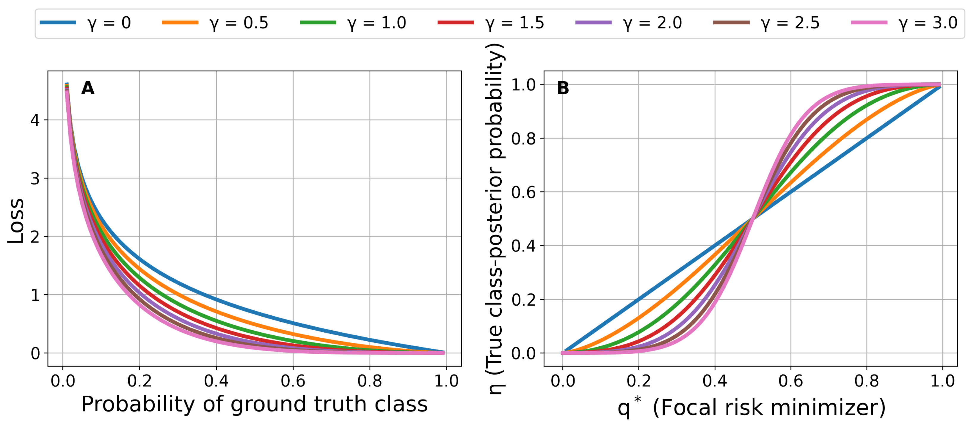
3.1. Focal Loss for Risk Prediction

The most common loss function used for risk prediction is the binary cross-entropy loss (also known as log loss or negative log-likelihood). The cross-entropy loss is a strictly proper loss function, and it is used to estimate the true class-posterior probability. It is also used as a surrogate loss function for classification. The cross-entropy loss is shown in Equation (1). For simplicity, we denote q ( x ) as q and η ( x ) as η :
l C E ( y , q ) = y log q ( 1 y ) log ( 1 q )
A loss function previously applied to classification tasks with imbalanced class labels is the focal loss, l F L γ . The focal loss was proposed in [24] for the object detection task in computer vision. It adds a modulating factor ( 1 q ) γ to l C E . The modulating factor is tuned by the focusing parameter, γ 0 . The binary focal loss is given by
l F L γ ( y , q ) = y ( 1 q ) γ log q ( 1 y ) q γ log ( 1 q )
A modulating factor with γ = 0 reduces the focal loss to the cross-entropy loss. A modulating factor with γ > 0 decreases the loss for “easy” samples. For example, suppose that the training sample ( x i , y i ) has the class label y i = 1 . The modulating factor decreases to 0 if the estimated confidence score for the training sample q i 1 . Therefore, the relative loss for the sample decreases to 0 and the training process shifts its focus to samples with erroneous confidence scores. The modulating effect of focal loss is enhanced for higher values of the focusing parameter γ . Figure 1A shows the modulation effect caused by the focusing parameter γ .
Unlike binary cross-entropy loss, focal loss is not a strictly proper loss function, and estimated confidence scores cannot be interpreted as reliable class-posterior probabilities [27]. A loss function, l : { 0 , 1 } × [ 0 , 1 ] R , is proper if η arg min q E Y l ( Y , q ) for every η [ 0 , 1 ] , where Y B e r n o u l l i ( η )  [28,41,42]. Furthermore, it is strictly proper if η is the unique minimizer.
The expected loss of a sample is the binary pointwise conditional risk given the prediction q and the true class-posterior probability η :
W l ( η , q ) = η l ( 1 , q ) + ( 1 η ) l ( 0 , q )
where l ( 1 , q ) and l ( 0 , q ) are partial losses. The binary pointwise conditional risk can be used to recover the true posterior probability, η , if the focal risk minimizer is available [27]. Let q * = arg min q W l F L γ ( η , q ) be the focal risk minimizer. Since focal loss is classification calibrated, then q * preserves the order of η : q i * < q j * η i < η j . Furthermore, the binary pointwise conditional risk with respect to focal loss, W l F L γ ( η , q * ) , is differentiable. To keep expressions simple, denote W l F L γ ( η , q * ) as W l F L γ , * ( η , q ) :
W l F L γ , * ( η , q ) = η ( ( 1 q ) γ log q ) + ( 1 η ) ( q γ log ( 1 q ) )
To find an expression for the class-posterior probability, the derivative of W l F L γ , * ( η , q ) with respect to q is set equal to 0:
d d q W l F L γ , * ( η , q ) = d d q η ( ( 1 q ) γ log q ) + ( 1 η ) ( q γ log ( 1 q ) ) = 0
Finally, the class-posterior probability given the focal risk minimizer is given by the following expression:
η = q γ 1 q γ q γ 1 log ( 1 q ) q γ 1 q γ q γ 1 log ( 1 q ) + ( 1 q ) γ q γ ( 1 q ) γ 1 log q η = Ψ γ ( q )
According to Equation (5), η = q if γ = 0 . Hence, l F L γ is strictly proper if and only if γ = 0 , i.e., when it is equal to l C E . However, η q if γ > 0 , i.e., l F L γ is not strictly proper if γ > 0 . The closed-form transformation Ψ γ : [ 0 , 1 ] [ 0 , 1 ] serves to calibrate a model trained via focal loss. The discriminatory power attained (often measured by the AUROC) through focal loss minimization is also maintained, since the transformation is a strictly increasing function. Therefore, the model gains calibration without losing discriminatory power. Figure 1B shows the relationship between the true class-posterior probability and the focal risk minimizer for different values of the focusing parameter γ . It should be emphasized that [27] initially introduces the transformation for the multiclass classification problem Ψ γ ( v ) = [ Ψ 1 γ ( v ) , . . . , Ψ K γ ( v ) ] T , where K is the number of classes, v is a K-dimensional simplex vector, Ψ i γ ( v ) = h γ ( v i ) l = 1 K h γ ( v l ) and h γ ( v ) = v ( 1 v ) γ γ ( 1 v ) γ 1 v log v . These equations are the result of a constrained convex program to optimize the pointwise conditional risk for the multiclass classification case. Equation (5) can be obtained from multiclass equations considering the case K = 2 and v = [ q , 1 q ] .
Applying the Ψ γ transformation is a necessary post-processing step to obtain the true class-posterior probability from the focal risk minimizer. Hence, the Ψ γ transformation is fundamental in the application of focal loss in risk prediction applications. However, statistical and machine learning models are trained to minimize a loss function over finite training datasets. Therefore, the loss function minimizer may not be obtained. In practice, even models such as logistic regression that minimize a strictly proper loss function may be miscalibrated [44]. Studies suggest adding a regularization term to the loss function to encourage better calibration of class-posterior probabilities [43,52].

3.2. Regularized GBDT

We employ regularized gradient-boosted decision trees (GBDT) to minimize a loss function. The training objective of the original GBDT is given by [11]:
L t = i = 1 n l ( y i , F t 1 ( x i ) + f t ( x i ) )
where l is a loss function, f t : X R is the t t h -decision tree, and F t 1 : X R is the ensemble model from iteration t 1 . Regularized GBDT such as XGBoost [13], LightGBM [14], and CatBoost [15] use the second-order Taylor expansion approximation to minimize the training objective:
L t i = 1 n [ l ( y i , F t 1 ( x i ) ) + g i f t ( x i ) + 1 2 h i f t 2 ( x i ) ] + Ω ( f t ) i = 1 n [ g i f t ( x i ) + 1 2 h i f t 2 ( x i ) ] + Ω ( f t )
where Ω ( f t ) is a regularization term to control the complexity of the decision tree, and g i = l ( y i , F t 1 ) F t 1 and h i = 2 l ( y i , F t 1 ) F t 1 2 are the first- and second-order derivatives of the loss function, respectively. The first- and second-order derivatives are known as gradient and Hessian, respectively. The right-hand side of Equation (7) can be rewritten as the weighted square loss, i = 1 n 1 2 h i ( f t ( x i ) + g i h i ) 2 + Ω ( f t ) + c o n s t a n t , with labels g i h i and weights h i , regularized by Ω ( f t ) . The goal in the t t h - iteration is to find the decision tree that minimizes this weighted loss. A class-posterior probability is obtained by applying the sigmoid transformation to the raw prediction of the ensemble model σ ( F ( x ) ) = 1 1 + e F ( x ) ( 0 , 1 ) . The gradient and Hessian of focal loss are derived in studies [16,18].

3.3. Bayesian Hyperparameter Optimization

Previous studies have suggested that Bayesian optimization outperforms random search, grid search, and manual search to tune the hyperparameters of gradient-boosted decision trees [53]. Bayesian optimization is capable of performing an informed search of hyperparameters to efficiently tune a machine learning model. Hence, in this study, we use the Bayesian optimization method known as sequential model-based optimization (SMBO) to tune hyperparameters [54,55]. SMBO uses a cheap surrogate model to evaluate an expensive black-box objective, g. Hyperparameters, λ , and losses, l, are stored as elements in a trajectory set, H = { ( λ i , l i ) } i = 1 T , to carry out an informed search of hyperparameters. In this study, we use the Gaussian process (GP) as a prior of g ( λ ) . An acquisition function is optimized using the posterior distribution of g ( λ ) given the trajectory set H to find the next hyperparameters to evaluate [56,57]. The acquisition function used in this study is the expected improvement:
E I ( λ ) = E [ max ( g ( λ b e s t ) g ( λ ) , 0 ) ]
where λ b e s t is the best hyperparameter combination obtained before the current iteration and λ is the next hyperparameter combination to evaluate by SMBO. This expectation is computed using the predictive mean and predictive variance of g ( λ )  [57].
Unlike previous studies on focal-aware gradient-boosted decision trees that used a balanced version of the focal loss and tuned hyperparameters to optimize g-mean or H-measure [18,19,20], we seek to tune hyperparameters to minimize the K-fold cross-validated focal loss on the training set. The reason is that the focal loss minimizer is necessary to obtain calibrated posterior probabilities after applying the Ψ γ transformation [27]. The Bayesian hyperparameter optimization procedure is shown in Algorithm 1:
Algorithm 1 SMBOFocalGBDT
Input:  M 0 , T, D f u l l _ t r a i n , focusing parameter γ , K
Output:  λ with minimum l F L γ , C V
1:
Initialize M 0
2:
H
3:
Divide D f u l l _ t r a i n into K stratified folds
4:
for  t { 1 , . . , T }   do
5:
     λ * arg min λ E I ( λ )            ▹ Minimize negative EI
6:
    for  k { 1 , . . . , K } do       ▹ Evaluate black-box objective
7:
         D k t r a i n j k D j
8:
         D k v a l D k
9:
        Train GBDT using D k t r a i n and hyperparameters λ *
10:
      Calculate validation focal loss l F L , k γ using D k v a l and Equation (2)
11:
     l F L γ , C V 1 K k = 1 K l F L , k γ        ▹ K-fold cross-validated focal loss
12:
     H H ( λ * , l F L γ , C V )
13:
    Fit M t to trajectory set H
Algorithm 1 depends on the selection of a focusing parameter γ . Since risk prediction models are evaluated in terms of discrimination and calibration, we will seek the focusing parameter γ that provides the GBDT with the best K-fold cross-validated Brier score on the training set. The Brier score, 1 n i = 1 n y i q ( x i ) 2 , is a strictly proper scoring rule and can be decomposed into discrimination and calibration components [9]. Therefore, the Brier score serves as a good metric for choosing the focusing parameter. We provide a second algorithm that describes the process of choosing the focusing parameter and selecting the final GBDT for risk prediction. Algorithm 2 trains different GBDTs via focal loss minimization with different γ and then selects the GBDT calibrated by Ψ γ transformation with the best K-fold cross-validated Brier score. Notice that this method is different from adjusting the focal loss parameter γ to directly optimize the Brier score. Here, we tune several models to minimize focal loss with predefined γ and then select the final clinical risk prediction model based on the Brier score.
Algorithm 2 Learning and Prediction Stages
Input:  M 0 , T, D f u l l _ t r a i n , focusing parameters { γ 1 , . . , γ e n d } , K, test sample x
Output: Prediction for test sample x
1:
for  γ { γ 1 , . . , γ e n d }   do
2:
     λ S M B O F o c a l G B D T ( M 0 , T , D f u l l _ t r a i n , γ , K )       ▹ Call Algorithm 1
3:
    Divide D f u l l _ t r a i n into K stratified folds
4:
    for  k { 1 , . . . , K }  do
5:
         D k t r a i n j k D j
6:
         D k v a l D k
7:
        Train GBDT using D k t r a i n and optimal hyperparameters λ
8:
        Calibrate confidence scores for D k v a l by Equation (5)
9:
        Calculate Brier score B S k γ for D k v a l by Equation (12)
10:
     B S γ , C V 1 K k = 1 K B S k γ        ▹ K-fold cross-validated Brier score
11:
     Γ Γ ( γ , B S γ , C V )             ▹ Track γ and B S γ , C V
12:
Train GBDT using D f u l l _ t r a i n , γ with minimum B S γ , C V , and optimal hyperparameters λ
13:
Estimate confidence score for test sample x
14:
Calibrate confidence score of test sample x using Equation (5)
GBDTs such as XGBoost and LightGBM provide a wide range of hyperparameters to prevent overfitting. Great differences in performance can be seen in GBDT with different hyperparameters due to the large number of possible combinations. Careful tuning of these hyperparameters is important in the context of clinical risk prediction applications. Large clinical databases pose several challenges, such as inaccurate data, noisy class labels, and high dimensionality (large number of features) [12]. Decision trees can easily overfit irrelevant patterns in clinical databases due to these problems. Decision trees are also biased towards numerical features. Numerical features provide more split values, leading to overfitting. We address these issues by carefully limiting the range of possible values for each hyperparameter. Nine hyperparameters are considered for XGBoost. These hyperparameters are learning rate, maximum tree depth, number of trees, fraction of samples in each tree, fraction of features in each tree, fraction of features in each tree level, l1 regularization, l2 regularization, and minimum sum of sample weights (Hessians) in each child node. Bayesian hyperparameter optimization starts with a distribution of possible values for each hyperparameter. We limit the learning rate to values between e 8 and e 2 . We choose these values to reduce the weights of each tree in the ensemble. However, small learning rates can possibly lead the Bayesian hyperparameter tuning process to increase the number of trees to overfit the validation dataset. Therefore, we also limit the total number of decision trees to the range [20, 300]. We use between 55% and 85% of the features in each decision tree to deal with high dimensionality. We also limit the total number of samples in each decision tree to the range [55%, 85%]. Random sampling of observations can decrease the variance of the ensemble and improve performance [58]. We limit the tree depth to values between 1 (decision stump) and 8. The l1 and l2 regularization parameters are used to shrink the values of the leaves. We search for a value in the space [ e 1 , e 6 ]. Larger values encourage sparsity and reduce leaf scores. The last hyperparameter is related to the sum of sample weights (Hessians) in a child node. The Hessian is the weight of each sample shown in the weighted square loss form of Equation (7). This hyperparameter is known as the “minimum child weight”. The “minimum child weight” hyperparameter stops tree growth if the sum of Hessians in a leaf is less than a threshold. We search for an appropriate threshold in the space [ e 1 , e 6 ]. Note that higher thresholds prevent overfitting.
Different distributions can be used in the Bayesian hyperparameter search. We select a discrete uniform distribution for the number of trees and the maximum tree depth. Uniform distributions are used for the maximum number of samples per tree, the fraction of features per tree, and the fraction of features per level. Log-uniform distributions are chosen for the remaining hyperparameters. These distributions are in part based on the distributions in the experimental setting described in [15]. This experimental setting was designed to compare XGBoost, LightGBM, and CatBoost. Appendix B provides the distribution of each hyperparameter used in the experiments.

3.4. Class-Imbalanced Classification Using Calibrated Focal-Aware GBDT

Rare outcomes and imbalanced class labels are ubiquitous in real clinical datasets. Common approaches to solving this problem include resampling to balance the frequency of class labels. Resampling approaches include oversampling observations from the minority class [59] and undersampling observations from the majority class. Potential problems with these techniques include miscalibrated posterior probabilities [60], the generation of synthetic minority samples that are likely to belong to the majority class [61], and the loss of information in the case of undersampling. In cases where the imbalance is extreme (e.g., malignancies after solid organ transplantation), resampling techniques would have to generate or discard a very large number of samples. Furthermore, these techniques do not optimize any specific classification metric or the cost of clinical intervention.
A simple approach to deal with class imbalance is to introduce class weights in the loss function [24]. Class weights equal to the inverse of the class frequencies can be multiplied by the relative losses. Another approach is to add margins or biases to the logits of the loss function. For example, adding margins equal to log 1 p ( y = 1 ) p ( y = 1 ) and log p ( y = 1 ) 1 p ( y = 1 ) to the logits of the positive and negative class samples in the logistic loss, log ( 1 + e y f ) , leads to Fisher consistency for the balanced error [38]. The Fisher consistency for balanced error guarantees an optimal balanced error in the large sample size limit. Minimizing this logit-adjusted loss encourages the model to optimize the balanced error. In recent years, logit adjusted losses have led to better classification performance in long-tailed deep learning [26] and in GBDT for the modeling of imbalanced bioassay data [17]. However, these methods consider misclassification costs during the training process and are not designed for risk prediction problems where the true class-posterior probabilities must be estimated.
A method of developing a classification rule using a clinical risk prediction model is threshold or logit adjustment after training. The threshold adjustment addresses the classification of class-imbalanced data by choosing a decision threshold that optimizes a classification metric or the cost of clinical intervention. The estimated posterior probabilities are then converted into binary labels [62]. Setting the decision threshold to the prior of the positive class, p ( y = 1 ) , optimizes the arithmetic mean of sensitivity and specificity [60,63,64]. This metric is known as the balanced accuracy. The prior probability, p ( y = 1 ) , is estimated using the relative frequency of the positive class, p ^ ( y = 1 ) n 1 n , where n 1 is the number of samples in the positive class, and n is the total number of samples in the training set. The success of probability thresholding depends on obtaining accurate class-posterior probabilities according to Theorem 1 in [60]. We provide the Theorem for the binary class-imbalanced problem for completeness:
Theorem 1
([60]). Let p ( y = 1 ) be the prior of class 1, and let η ( x ) = p ( y = 1 | x ) be the true class-posterior probability. If the proportion of the minority class label in the testing set is equal to the proportion of the minority class label in the training set, then
δ ( x )   : = 1 , if η ( x ) p ( y = 1 ) > 1 η ( x ) 1 p ( y = 1 ) 0 , O t h e r w i s e
maximizes the balanced accuracy.
Theorem 1 provides a method to maximize balanced accuracy (or minimize balanced error) after training. Equation (9) is a cost-weighted Bayes rule, 1 ( c ( 0 , 1 ) η ( x ) > c ( 1 , 0 ) ( 1 η ( x ) ) ) , with costs of misclassification c ( 0 , 1 ) = 1 p ( y = 1 ) and c ( 1 , 0 ) = p ( y = 1 ) . In this expression, c ( 0 , 1 ) is the cost of classifying a positive sample as negative, and c ( 1 , 0 ) is the cost of classifying a negative sample as positive [63,65]. This classifier assumes that the costs of misclassification are much higher for positive samples when the data set has imbalanced class labels ( p ( y = 1 ) < < 0.5 ). A rearrangement of the condition in (9) leads to the optimal decision threshold for the balanced accuracy to be p ( y = 1 ) . In practice, we have the model’s estimated class-posterior probabilities and the relative frequency of the positive class in the training set p ^ ( y = 1 ) . Therefore, the goal is to estimate accurate class-posterior probabilities to optimize the balanced accuracy. Collel. et al. previously investigated the combination of threshold adjustment with bagging classifiers [60]. In this study, we investigate the performance of GBDT trained via focal loss and the empirical threshold equal to the relative frequency of the positive class in the training set:
δ ^ ( x )   : = 1 , if Ψ γ ( q ( x ) ) > p ^ ( y = 1 ) 0 , O t h e r w i s e
where Ψ γ ( q ( x ) ) is the calibrated confidence score of a model trained by minimizing the focal loss (5). This method has advantages in the context of clinical risk prediction. The model should provide calibrated class-posterior probabilities assuming the focal loss minimizer is learned. Then, Equation (10) optimizes both sensitivity and specificity without threshold optimization. The classifier solely depends on having accurate estimates of the class-posterior probabilities and a consistent estimator of the prior probability of the minority class. Other decision thresholds can be used assuming the class-posterior probabilities are well calibrated. Different decision thresholds may optimize costs associated with clinical interventions [9] or classification metrics such as the F1-score [66].

3.5. Evaluation Metrics

This section introduces the evaluation metrics used in this study. We describe discrimination, calibration, and classification metrics to evaluate risk prediction and classification models. The discrimination metrics used in this study are the AUROC and the H-measure. The receiver operating characteristic (ROC) curve displays the true positive rate ( T P R ) and the false positive rate ( F P R ) for different decision thresholds. The AUROC is 1 when the model ranks all positive samples higher than negative samples. The AUROC is 0.5 if the model cannot separate positive samples from negative samples; that is, the model provides a random guess. The AUROC is given by the following expression:
A U R O C = 0 1 T P R ( F P R ) d F P R
The H-measure metric is also defined over the ROC curve and considers misclassification costs by incorporating a misclassification severity distribution [7,67]. The average precision is also considered. The average precision measures the area under the precision–recall curve, which is useful for comparing classifiers trained with class-imbalanced data. The precision–recall curve provides precision and recall, or TPR, for different decision thresholds. The average precision is calculated as the weighted mean of precision values for different decision thresholds. Each weight is the increase in the recall with respect to the recall value obtained using the previous decision threshold.
To assess calibration, we used the Brier score. The Brier score is the mean squared error for predicted probabilities and it is a strictly proper scoring rule:
B r i e r s c o r e = 1 n i = 1 n y i q ( x i ) 2
The best possible Brier score for a model is 0. The Brier score measures both calibration and discrimination, so it serves as an overall accuracy metric. Therefore, we also used the calibration plot to visualize the calibration of the predicted probabilities. We use quantile binning to assign predicted probabilities to groups. The predicted probabilities are sorted and grouped into 10 bins, each with the same number of samples. The fraction of positive samples and the mean predicted probability are then plotted for each bin. A perfect calibration curve must be aligned with the line of identity. We also provide the calibration slope and intercept to quantify calibration. The calibration slope and intercept are extracted from a logistic regression model that uses the logit of the predicted posterior probabilities as an independent variable and the binary outcome as a dependent variable. The coefficient and intercept are the calibration slope and the calibration intercept, respectively. A risk prediction model is calibrated if the calibration slope and intercept are equal to 1 and 0, respectively. The predicted posterior probabilities are then considered to be in agreement with the positive label frequencies in the test data. The deviation from these values indicates miscalibration. The calibration slope and intercept are commonly used to assess models in the clinical risk prediction literature [8,10,35,68].
To assess classification performance, we used sensitivity (recall or TPR), specificity or true negative rate (TNR), and balanced accuracy or arithmetic mean of sensitivity and specificity. These metrics measure the proportion of samples correctly classified. The metrics are expressed as follows:
S e n s i t i v i t y ( T P R ) = T P T P + F N
S p e c i f i c i t y ( T N R ) = T N T N + F P
B a l a n c e d a c c u r a c y = T P R + T N R 2
where TP stands for true positives, TN are true negatives, FP are false positives, and FN are false negatives. These metrics depend on the selection of a decision threshold to convert the class-posterior probabilities into class labels.
This study used data from the Scientific Registry of Transplant Recipients (SRTR) [69]. The SRTR data system includes data on all donors, wait-listed candidates, and transplant recipients in the US, submitted by members of the Organ Procurement and Transplantation Network (OPTN). The Health Resources and Services Administration (HRSA), US Department of Health and Human Services, provides oversight to the activities of the OPTN and SRTR contractors.

4. Experiments

This section describes lung transplantation data from the Scientific Registry of Transplant Recipients (SRTR) and the Behavioral Risk Factor Surveillance System (BRFSS) of the Centers for Disease Control and Prevention (CDC). The first application consists of cancer prediction in lung transplant recipients. The second application consists of the prediction of diabetes based on survey responses from residents of the United States. The experimental settings and results are described in detail.

4.1. Datasets

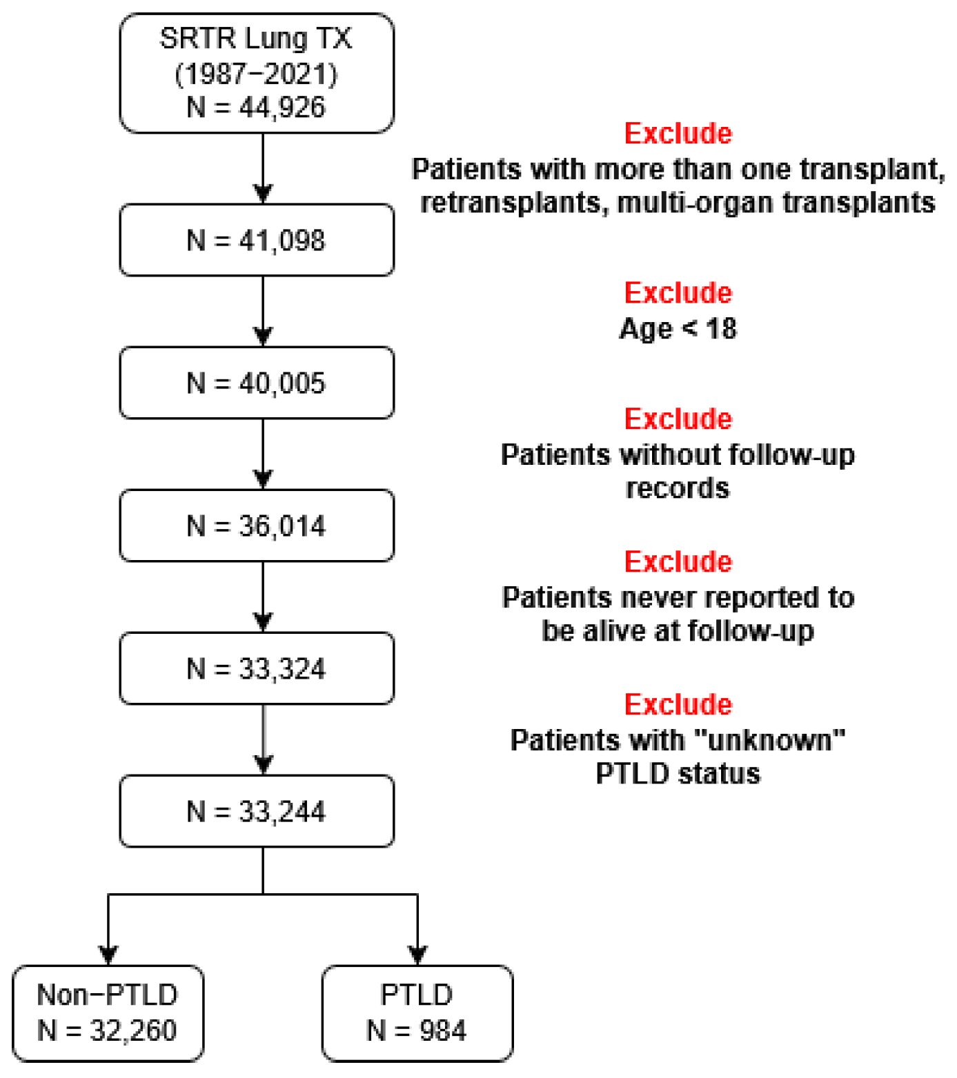
4.1.1. Lung Transplant Data

SRTR has stored data on solid organ transplant candidates, recipients, and donors in the United States since 1987. Its primary source is the Organ Procurement and Transplantation Network (OPTN). Solid organ transplants in the registry consist of the heart, lung, kidney, pancreas, liver, and intestines. SRTR files provide features related to demographics, medical history, immunosuppression, histocompatibility, donor–recipient matching, transplant follow-up, and outcomes including death and malignancy after transplantation.
The initial lung transplant file contains 44,926 patients from 16 October 1987, to 1 June 2021. We extract lung transplant recipients from the SRTR and filter the data using the exclusion criteria shown in Figure 2. We exclude patients with retransplantation, patients under 18 years of age, patients without follow-up records, and patients with unknown cancer status. The final dataset includes 33,244 patients from 1 January 1988 to 28 November 2020. The binary outcome is post-transplant lymphoproliferative disorder (PTLD). PTLD is a malignancy that occurs in solid organ transplant recipients [70]. It is one of the most common malignancies after non-melanoma skin cancer among lung transplant recipients. The mortality range for lung transplant recipients who develop PTLD is 20–50% [71]. The status and type of malignancy are extracted from the SRTR malignancy file. We calculate the time-to-PTLD by subtracting the date of diagnosis of PTLD from the date of transplantation. The final number of patients is 33,244 with 32,260 (97.04%) patients who did not develop PTLD and 984 (2.96%) patients who developed PTLD. We then generate datasets with binary outcomes for five different time horizons: 1, 3, 5, 8, and 10 years. Patients who were not followed up or died during the period of time were excluded. Patients who developed PTLD before the end of the time horizon are assigned an outcome of 1, while patients who did not develop PTLD before the end of the time horizon are assigned an outcome of 0. The numbers of patients are 28,883, 19,501, 13,351, 7507, and 5159 for 1, 3, 5, 8, and 10 years after transplantation, respectively. The datasets show a high degree of class-imbalance. The relative frequencies of the event are 1.14%, 2.92%, 5.19%, 10.87%, and 17.02% for 1, 3, 5, 8, and 10 years after transplantation, respectively. We consider features including demographics, immunosuppression during transplantation and early post-transplantation period (medications for induction and anti-rejection), viral infections prior to transplantation, and some of the most common human leukocyte antigens (HLA) among lung recipients. A total of 54 features are used to predict PTLD in lung transplant recipients. Feature names and basic statistics are shown in Table A1 and Table A2 of Appendix A. Two of the 54 features are numerical. The remaining features are categorical. We perform a Wilcoxon rank sum test to compare numerical features of cancer and non-cancer patients. The Wilcoxon rank sum test is a non-parametric statistical test that compares the locations of two distributions. The p-values of the statistical test are available in Table A1 of Appendix A. We also perform a chi-square test to compare categorical features of cancer and non-cancer patients. The test is performed to assess whether there is an association between categorical features and the outcome. The contingency tables and p-values are available in Table A2 of Appendix A. These statistical tests are performed as preliminary analyses of the features. Figure 3 shows the distributions of six features used to predict PTLD.

4.1.2. Diabetes Data

We also use data from the Behavioral Risk Factor Surveillance System (BRFSS) [72]. The BRFSS is a survey collection data system established by the Centers for Disease Control and Prevention (CDC) in 1984. It collects data from residents of the United States related to demographics, risky living habits, healthcare coverage, chronic, and infectious diseases. More than 400,000 surveys are conducted by telephone in 50 states of the US every year. We utilize the pre-processing pipeline available in [73]. The pipeline extracts 253,680 survey responses without missing values from the 2015 file available in [74]. We obtained 229,474 samples after removing duplicated rows.
The binary outcome for the BRFSS dataset is diabetes (including pre-diabetes). The relative frequency of the event is 15.29%. There are 21 features in total. These features are extracted from the survey responses. Each survey represents a row or sample. Three of the 21 features are numerical features. Numerical features include body mass index, number of days with poor mental health (in a 30-day window), and number of days with poor physical health (in a 30-day window). The remaining features are categorical. These features are related to high blood pressure, high cholesterol, smoking, stroke, alcohol consumption, heart disease, demographics (sex, age group, education, and income), healthcare coverage, and eating habits (fruit and vegetable consumption per day). Wilcoxon rank sum test was performed to compare the numerical features of residents with diabetes and residents without diabetes. Chi-square test was performed to compare categorical features. The names of features, means, standard deviations, and categories are shown in Table A3 and Table A4. Figure 4 shows the distributions of six features used to predict diabetes.

4.2. Design of Experiments
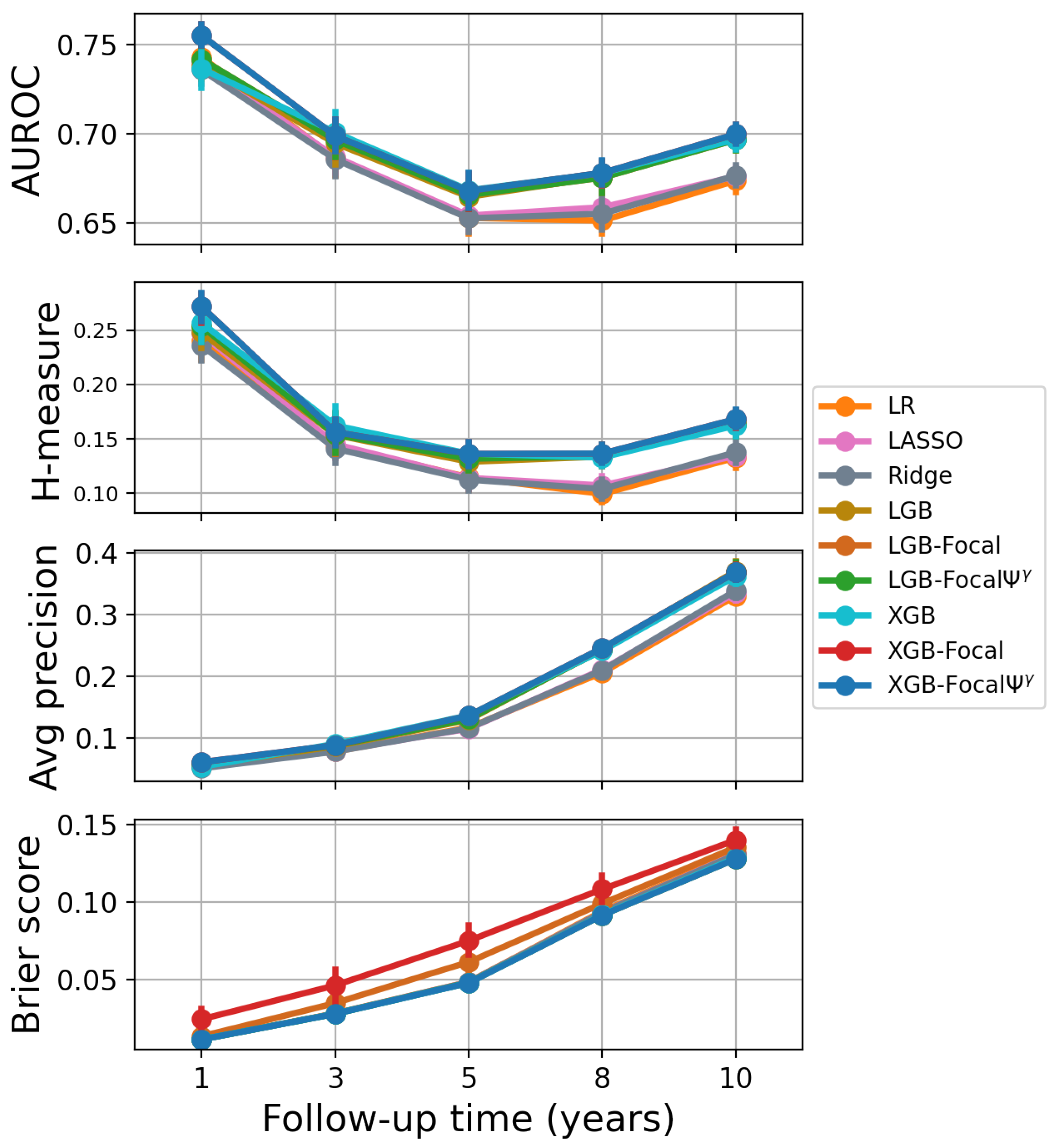
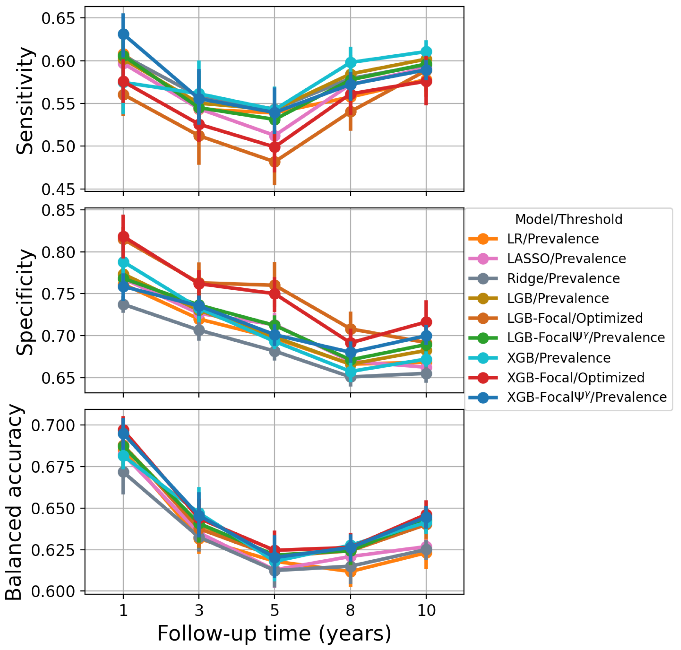
Each dataset is split into a training set (70%) and a testing set (30%). Median and mode imputations are performed for continuous and categorical features with missing values, respectively. We consider several statistical and machine learning models for comparison, including logistic regression (LR) without regularization, LR with least absolute shrinkage and selection operator (LASSO) regularization, LR with ridge regularization, LightGBM, XGBoost, LightGBM-Focal, and XGBoost-Focal. LR models are chosen because they are commonly used in clinical risk prediction applications. We compare the performance of focal-aware GBDT before and after applying the Ψ γ transformation. We also apply Platt scaling [45] and isotonic regression [47] to the predictions of GBDT trained using focal loss. For these heuristic techniques, we use 10-fold cross-validation over the training set to generate a new set consisting of miscalibrated predictions and true class labels. We then fit sigmoid and isotonic regression models to this new set. Note that miscalibrated predictions are converted into logits, and true labels are scaled to 1 n 0 + 2 , n 1 + 1 n 1 + 2 for the Platt scaling method [45]. We provide the expression of the sigmoid transformation used in the Platt scaling:
q P l a t t = 1 1 + e A l o g i t ( q ) + B
where l o g i t ( q ) is the logarithmic odds of prediction q, and A and B are the hyperparameters to be tuned to improve the calibration. The output q P l a t t is the calibrated probabilistic prediction.
All models are tuned with Bayesian hyperparameter optimization with T = 30 iterations. Hyperparameters are selected to minimize the 10-fold cross-validated cross-entropy loss for all models except for models trained through focal loss. The focal loss parameter is initially set to 0.1, and then the parameter search continues from 0.25 to 2.5 with a step size of 0.25. The distributions of other hyperparameters considered are provided in Appendix B. The scikit-learn [75], LightGBM, XGBoost, scikit-optimize, statsmodels, and hmeasure packages are used for model development, hyperparameter tuning, and evaluation. Algorithms 1 and 2 are used to train all models that used focal loss as a loss function.
We use the relative frequency of the minority class label (prevalence) as the decision threshold for calibrated models. In addition, we also use an optimized decision threshold for the miscalibrated GBDT models trained using focal loss. An optimized threshold is used because the posterior probabilities produced by these models are not accurate. Therefore, the prevalence threshold will not optimize balanced accuracy according to Theorem 1 in Section 3.4. To find the optimized threshold, we train the model with optimal hyperparameters and perform 10-fold cross-validation again. For each iteration of 10-fold cross-validation, we find the best decision threshold that optimizes the balanced accuracy in the validation fold. Finally, the mean of these ten thresholds is used as the final decision threshold to perform the classification in the test set.
Risk probabilities are plotted to show the calibration of models trained using focal loss. We provide calibration plots based on quantile binning with 10 bins. The described experiment is repeated 10 times for the PTLD dataset using different random seeds. For the prediction of diabetes using the BRFSS, we performed only three rounds of cross-validation due to the large size of the dataset. We provide the mean performance over the three cross-validation experiments.

4.3. Results

The mean γ values for the 10 experiments for the XGBoost-Focal models are 1.49, 1.34, 1.63, 1.10, and 0.92 for the prediction of the risk of PTLD at 1, 3, 5, 8, and 10 years, respectively. The mean γ values for the 10 experiments for the LightGBM-Focal models are 0.60, 0.85, 1.05, 0.65, and 0.61 for the prediction of the risk of PTLD at 1, 3, 5, 8, and 10 years, respectively. The γ value for each repetition of shuffled cross-validation is automatically selected by Bayesian hyperparameter optimization (Algorithms 1 and 2). Higher γ values deteriorate the calibration. Table 1, Table 2 and Table 3 and Figure 5 and Figure 6 show the model performance for the prediction of PTLD in lung transplant recipients. From Table 1, we observe that AUROC, the H-measure, and the average precision are the same for GBDT-Focal before and after applying the Ψ γ transformation. GBDT-Focal combined with Platt scaling also preserves the same discriminatory power. This result is expected because the Ψ γ and sigmoid transformations (used in Platt scaling) preserve the order of the confidence scores. Therefore, ranking metrics such as AUROC, H-measure, and average precision remain unchanged.
Table 2 and Figure 5 show that the Ψ γ transformation improves the performance of XGBoost-Focal and LightGBM-Focal according to the Brier score. All calibrated XGBoost-Focal models show an overall improved accuracy according to the Brier score metric compared to their miscalibrated counterparts. The Brier scores for XGBoost-Focal are 0.0242, 0.0460, 0.0749, 0.1082, and 0.1400 for years 1, 3, 5, 8, and 10, respectively. The Brier scores for XGBoost-Focal Ψ γ are 0.0110, 0.0277, 0.0476, 0.0914, and 0.1278 for years 1, 3, 5, 8, and 10, respectively. Since discrimination remains unchanged, the improvement in the Brier score can be attributed to an improvement in the calibration of the confidence scores.
Figure 7 and Figure 8 display calibration plots for different time horizons. As seen in the leftmost columns, both XGBoost and LightGBM trained via focal loss minimization overestimate the risks of PTLD post-transplantation across all time horizons. For example, the group with the lowest risk during the first year after transplantation (first bin in the first subplot of XGBoost-Focal in Figure 7) has a mean predicted probability of 0.0758, while the actual risk is 0.002. Furthermore, the group with the highest post-transplant risk during the first year has a mean predicted probability of 0.185 while the actual risk is 0.052. In contrast, calibration of the XGBoost models trained via focal loss is greatly improved across all time horizons after applying the Ψ γ transformation. The mean predicted probabilities of the lowest and highest risk groups for the first year are 0.0035 and 0.044 after applying the Ψ γ transformation, respectively. All post-processing methods improve the calibration with respect to the raw GBDT trained through focal loss. However, GBDT calibrated using isotonic regression shows worse performance, as reflected by the higher Brier score in Table 2. The poor performance might be due to the small number of positive samples available in the lung transplant dataset.
The calibration slope and intercept were also calculated to quantify the calibration plots. These values are shown as box plots in Figure 9. The ideal values for the calibration slope and intercept are 1 and 0 (shown as red horizontal lines in both subplots), respectively. The median calibration slope and intercept for XGBoost-Focal for the prediction of 1-year risk of PTLD are 2.744 (interquartile range (IQR): 1.787–3.196) and 0.654 (IQR: 0.282–0.829), respectively. These values indicate that XGBoost-Focal is severely miscalibrated. The median calibration slope and intercept for the XGBoost-Focal calibrated using the Ψ γ transformation are 1.138 (IQR: 1.041–1.192) and 0.563 (0.262–0.772), respectively. The median calibration slope and intercept for the XGBoost-Focal calibrated using Platt scaling are 1.066 (IQR: 1.009–1.113) and 0.272 (IQR: 0.032–0.486), respectively. The median calibration slope and intercept for the XGBoost-Focal calibrated using isotonic regression are 0.986 (IQR: 0.892–1.043) and −0.048 (IQR: −0.436–0.160), respectively. The median calibration slope and intercept for XGBoost-Focal for the prediction of 10-year risk of PTLD are 1.579 (IQR: 1.217–1.941) and −0.040 (IQR: −0.081–0.104), respectively. The median calibration slope and intercept for the XGBoost-Focal calibrated using the Ψ γ transformation are 0.968 (IQR: 0.917–1.040) and −0.045 (IQR: −0.088–0.099), respectively. The median calibration slope and intercept for the XGBoost-Focal calibrated using Platt scaling are 0.969 (IQR: 0.932–1.058) and −0.026 (IQR: −0.137–0.114), respectively. The median calibration slope and intercept for the XGBoost-Focal calibrated using isotonic regression are 0.848 (IQR: 0.802–0.935) and −0.224 (IQR: −0.297–(−0.110)), respectively. The calibration slopes and intercepts for the remaining time horizons are shown in Figure 9.
XGBoost trained using focal loss achieved better discrimination compared to standard XGBoost to predict cancer one year after lung transplantation. The AUROC values are 0.755 and 0.736 for XGBoost-Focal and standard XGBoost, respectively. The H-measure values are 0.271 and 0.257 for XGBoost-Focal and standard XGBoost, respectively. These values are shown in Table 1 and Figure 5. XGBoost-Focal calibrated using the Ψ γ transformation achieved the best sensitivity (0.631) to predict cancer one year after transplantation, as shown in Table 3 and Figure 6. The discriminatory power and the overall accuracy (in terms of the Brier score) of XGBoost-Focal and XGBoost trained using cross-entropy loss are comparable in the remaining time periods. The differences in AUROC between the best GBDT model and the best logistic regression are in the range 0.007–0.023 for all risk prediction tasks (including diabetes prediction). Differences in the H-measure and average precision are more prominent. The differences between the best GBDT model and the best logistic regression are in the range of 0.013–0.031 for the H-measure and 0.006–0.035 for the average precision. XGBoost also tended to perform slightly better than LightGBM in all prediction tasks.
In summary, the XGBoost-Focal Ψ γ models are equally competitive or better than other models according to the AUROC, H-measure, average precision, and Brier score across all time horizons. We observe that GBDT models achieve better performance compared to logistic regression models (unregularized and regularized) as the time horizon increases for the prediction task, as evidenced by the H-measure and average precision of the models. Figure 5 displays the performance of the risk prediction models as the time horizon changes.
The thresholded classification metrics of all models, including sensitivity and specificity, are provided in Table 3. Models trained with focal loss are overconfident, that is, they assign a higher probability of event. As a result, the prevalence threshold would convert most confidence scores to positive labels, leading to a perfect or nearly perfect sensitivity but low specificity. This problem is solved using an optimized threshold or by calibrating confidence scores before using the prevalence as a decision threshold, as discussed in Section 3.4 (Equation (10)). In addition, we observe that optimized decision thresholds provide comparable or slightly better balanced accuracy at the expense of lower sensitivity and higher specificity. We notice this trend for both LightGBM-Focal and XGBoost-Focal through different time horizons in the PTLD prediction task (see Table 3 and Figure 6). We also find that the sensitivity values of LightGBM-Focal and XGBoost-Focal using the optimized thresholds tend to be worse than the sensitivity values achieved by the models using the prevalence threshold. This is not desirable, as positive samples are associated with higher costs of misclassification in clinical risk prediction applications. Therefore, the prevalence threshold is more appropriate than the optimized balanced accuracy threshold in the PTLD prediction task.
Figure 10 shows the calibration plots for the diabetes prediction task. The mean values of γ across the three shuffled cross-validation experiments are 1.03 for LightGBM-Focal and 1.08 for XGBoost-Focal. LightGBM-Focal and XGBoost-Focal show equal miscalibration. All post-processing methods successfully calibrate the predicted probabilities, as shown in Figure 10 (mean predicted probabilities and fraction of positives in the test set match). Isotonic regression provides almost equal performance to the other calibration methods thanks to the larger sample size. Table 4 provides the AUROC, H-measure, average precision, and Brier score for the diabetes prediction task. We observe that the calibrated XGBoost-Focal and the standard XGBoost have a mean Brier score equal to 0.1052. In general, the differences between GBDT trained using focal loss and GBDT trained using cross-entropy loss are less prominent in the diabetes prediction task. The classification metrics for the diabetes prediction task are provided in Table A5 of the Appendix C.

5. Discussion

This study investigated the impact of focal loss in the context of clinical risk prediction. Although existing studies have combined GBDT with custom loss functions [16,17,18,19,20,21,22,23,39], few have addressed the topic of probability calibration. Probability calibration assesses the accuracy of the confidence scores provided by a model. The confidence scores represent the predictive uncertainty of the model. Miscalibrated posterior probabilities can be misleading for decision-making tasks [10]. This is because miscalibrated scores do not represent the fraction of positive observations for a given set of features. We proposed a method to select the focusing parameter of the focal loss function to optimize discrimination and calibration. The method was based on the Ψ γ transformation proposed in [27] and Bayesian hyperparameter optimization. Our study also uses calibration plots and the Brier score to assess the effect of the transformation and the “overall accuracy” (discrimination plus calibration), respectively. Probability calibration plots and the Brier score are popular in the clinical risk prediction literature [8,9]. These calibration metrics have attracted attention in recent deep learning research related to calibration [44,76].
Since focal loss is not strictly proper, minimization does not lead to true class-posterior probabilities. Therefore, confidence scores should not be interpreted as accurate clinical risks unless a transformation is applied after training. The transformation applied in the experiments directly related the focal loss minimizer to the true class-posterior probability. Such a transformation may not exist for all loss functions. For example, class-posterior probability estimation is not possible for some asymmetric losses [52] and for the hinge loss [45,77]. Models trained using these losses require heuristic techniques such as Platt scaling and isotonic regression. These techniques increase computational time and require a calibration dataset or cross-validation to prevent overfitting. Isotonic regression can also produce poor calibration for small sample sizes.
In our experiments, we have observed that miscalibrated GBDTs trained via focal loss minimization produce overconfident predictions. The overconfidence can be seen in the mean predicted probabilities of XGBoost-Focal and LightGBM-Focal in Figure 7, Figure 8 and Figure 10. The mean predicted probabilities before calibration (horizontal axis) are greater than the fraction of positives (vertical axis) in the test dataset. The plotted bins were below the identity line, indicating overestimated risks [10]. However, models trained through focal loss can also produce underconfident predictions. This phenomenon was first observed in deep neural networks trained using focal loss [76] and was later formalized in [27]. Mukhoti et al. used this property and proposed a method to find focusing parameters to calibrate overconfident deep neural networks [76].
The use of isotonic regression resulted in a worse performance than using the Ψ γ transformation or Platt scaling in the prediction of PTLD (see the higher Brier score and lower average precision for 5, 8, and 10 year cancer prediction in Table 2 and Table 1, respectively). The most likely explanation is that the isotonic regression is sensitive to data imbalance and that a small number of positive cancer patients leads to poor performance. Furthermore, isotonic regression did not maintain the discriminatory power of the model. This is because the isotonic regression fits a step-wise isotonic function instead of a strictly increasing function [47]. This approach introduces ties between similar probabilities and changes ranking metrics such as the AUROC, the H-measure, and the average precision. Unlike isotonic regression, the Ψ γ transformation and sigmoid transformation (used in Platt scaling) are strictly increasing. Hence, they do not alter the discrimination of the model, as shown in the AUROC and H-measure metrics in Table 1 and Table 4. Isotonic regression achieved performance comparable to other calibration methods in the prediction of diabetes (see Brier scores in Table 4). Note that the diabetes dataset contains more positive observations compared to the lung transplant dataset.
An advantage of choosing focal loss over the strictly proper cross-entropy loss in clinical risk prediction applications is its flexibility. Focal loss forces the training process to “focus” on hard-to-classify samples, thanks to its focusing parameter. This parameter can prove useful when dealing with large medical databases with imbalanced classes or rare samples (samples with large losses). As an example, we found that XGBoost and LightGBM trained using focal loss achieved better discrimination compared to standard XGBoost and LightGBM for cancer prediction one year after lung transplantation. XGBoost-Focal ( Ψ γ ) also achieved a higher sensitivity compared to other models for the same time horizon as shown in Table 3. However, it is important to emphasize that focal loss might not always enhance performance. GBDT trained with focal loss and cross-entropy loss had an equal Brier score and an almost equal AUROC in the diabetes prediction application (Table 4). Therefore, forcing the training process to focus on rare samples is not necessary for every dataset or application. The focusing parameter γ = 0 can be considered to tune the GBDT using Algorithms 1 and 2. A focusing parameter γ = 0 will handle cases for which the cross-entropy loss would lead to better performance. In this case, the transformation Ψ γ is no longer necessary because the loss is strictly proper, as explained in Section 3.1.
This study also explored threshold adjustment in combination with GBDT trained using focal loss. Many applied machine learning studies assume a regular decision threshold of 0.5. In this setting, minimization of weighted cross-entropy loss or logit-adjusted loss is necessary to maximize balanced accuracy. Boldini et al. previously studied these loss functions in combination with GBDT [17]. A model trained through weighted cross-entropy loss or logit-adjusted loss will provide balanced class-posterior probabilities [38]. Note that balanced posterior probabilities would overestimate the risks or true posterior probabilities. Therefore, these loss functions are mainly applicable to classification problems. We specifically used the prevalence threshold to maximize balanced accuracy after applying the transformation Ψ γ . The choice of decision threshold is based on Theorem 1 provided by Collel et al. in [60]. This decision threshold optimizes the balanced accuracy in the large sample size limit given accurate posterior probabilities. This threshold would fail to optimize the balanced accuracy without a calibration step because the probabilities estimated using focal loss are not reliable. Therefore, an optimized threshold is needed when the Ψ γ transformation or a heuristic technique is not applied. Note that estimation of the optimized threshold would increase the computational burden since it would require K-fold cross-validation to prevent overfitting.
A limitation observed in the experiments is that the selected focusing parameter may not be the same for cross-validation repetitions with different random seeds. This is evident in Figure 7, Figure 8 and Figure 10. The background curves show different degrees of miscalibration caused by training XGBoost-Focal and LightGBM-Focal with different focusing parameters. These focusing parameters were chosen automatically in the Bayesian hyperparameter tuning stage, as described in Section 3.3. A possible explanation is that the heterogeneity of the patient groups available in the SRTR database (including patient groups from different transplant centers and time periods) causes different focusing parameters to be selected for different cross-validation repetitions. Problems such as label noise may also cause hyperparameter values to fluctuate among different cross-validation runs. These observations are consistent with studies showing that the hyperparameter tuning of GBDT is sensitive to noise in electronic health records [12]. For model deployment, it is recommended to estimate this parameter using the full dataset after assessing stability through repeated cross-validation runs.
A limitation of our experimental setting is that we did not consider other GBDT models in addition to XGBoost and LightGBM. Other variants of GBDT include CatBoost [15] and PaloBoost [12]. PaloBoost is a variant of the original stochastic GBDT model [58]. PaloBoost is designed to be less sensitive to hyperparameter settings. CatBoost introduces an algorithm to automatically handle categorical features. Clinical databases such as the SRTR typically contain many categorical and ordinal features. Hence, CatBoost can be used as an alternative to XGBoost and LightGBM in clinical risk prediction applications. We also did not consider recent hyperparameter optimization techniques to tune GBDT [78]. A future research direction is to explore CatBoost and novel hyperparameter optimization techniques in combination with custom loss functions.

6. Conclusions

This paper investigated focal loss in clinical risk prediction problems. We investigated the application of a closed-form transformation ( Ψ γ transformation) to calibrate the confidence scores of XGBoost and LightGBM trained using focal loss. Algorithms based on Bayesian hyperparameter tuning were proposed to select the focal loss parameter to optimize discriminatory power and calibration. Adjustment of the decision threshold was also investigated to optimize the balanced accuracy classification metric. We considered two real-life applications related to lung transplantation and diabetes prediction.
The methods and experiments presented in this study can support the adoption of the focal loss function to train clinical risk prediction models. The practical implications of improving clinical risk prediction include providing data-driven models to support clinical professionals, standardize patient care, accelerate clinical decision making to prioritize treatment, and improve patient outcomes through preventive interventions. Despite the benefits of machine learning techniques for clinical risk prediction, there are ethical concerns that require attention. Although the gradient-boosted decision tree model can potentially improve predictive performance compared to conventional statistical approaches, it can also inherit biases present in the training data. These biases are more difficult to detect in complex models such as GBDT than in simpler linear models. Therefore, extensive validation is essential to detect and minimize biases. Interpretable approaches also need to be thoroughly explored to support the adoption of GBDT and new loss functions in high-stakes clinical decision making.
A future research direction is to explore the application of focal loss in the field of fair machine learning. Focal loss can be applied to improve predictive performance in tasks with underrepresented or minority groups in electronic health records. The focal loss parameter can be used to reduce the loss of a sample of a minority group in a medical database. Custom loss functions can be developed to correct biases in GBDT for clinical risk prediction. Another direction for future research is to use focal loss and logit-adjusted losses to train GBDT for multiclass and multilabel classification.

Author Contributions

Conceptualization, N.N. and D.D.; Methodology, H.J. and D.D.; Validation, H.J.; Formal analysis, H.J.; Data curation, N.N.; Writing—original draft, H.J.; Writing—review & editing, D.D.; Supervision, N.N. and D.D.; Project administration, D.D. All authors have read and agreed to the published version of the manuscript.

Funding

This research received no external funding.

Data Availability Statement

The Scientific Registry of Transplant Recipients (SRTR) database is publicly available through the SRTR (https://www.srtr.org). The database is subject to the data use agreement. Behavioral Risk Factor Surveillance System (BRFSS) files are publicly available through the Centers for Disease Control and Prevention (CDC). The files can be accessed via https://www.cdc.gov/brfss/annual_data/annual_data.htm (accessed on 24 July 2024). The diabetes dataset is available at: https://www.kaggle.com/datasets/alexteboul/diabetes-health-indicators-dataset/data (accessed on 24 July 2024).

Acknowledgments

The data reported here have been supplied by the Hennepin Healthcare Research Institute (HHRI) as the contractor for the Scientific Registry of Transplant Recipients (SRTR). The interpretation and reporting of these data are the responsibility of the author(s) and in no way should be seen as an official policy of or interpretation by the SRTR or the U.S. Government.

Conflicts of Interest

The authors declare no conflicts of interest.

Appendix A. Feature Description

For the Scientific Registry of Transplant Recipients (SRTR), the body mass index variable ( R E C _ B M I ) was converted into a categorical feature with four groups: underweight, normal, overweight, and obese. Patients with a R E C _ B M I less than 18.5 are labeled as “underweight”. Patients with 18.5 R E C _ B M I < 25 are labeled “normal”. Patients with 25 R E C _ B M I < 30 are labeled as “overweight”. Patients with R E C _ B M I 30 are labeled “obese”.
Table A1. Numerical features from post-transplant lymphoproliferative disorder (PTLD) dataset extracted from the SRTR files. Wilcoxon rank sum test was performed to compare numerical features.
VariableTotal Mean (SD)PTLD Negative Mean (SD)PTLD Positive Mean (SD)p-Value
REC_AGE_AT_TX54.81 (12.86)54.91 (12.80)51.51 (14.20)0
DON_AGE33.73 (13.89)33.79 (13.90)31.74 (13.35)0
Table A2. Categorical features from post-transplant lymphoproliferative disorder (PTLD) dataset extracted from the SRTR files. Chi-square test was performed to compare categorical features.
VariableCategoryTotalPTLD NegativePTLD Positivep-Value
REC_BMI_CATNormal13,47013,0684020.000
REC_BMI_CATObese482647111150.000
REC_BMI_CATOverweight11,49311,1713220.000
REC_BMI_CATUnderweight301528881270.000
REC_A_MM_EQUIV_TX022402172680.605
REC_A_MM_EQUIV_TX112,47212,1313410.605
REC_A_MM_EQUIV_TX214,83314,4034300.605
REC_B_MM_EQUIV_TX0621595260.072
REC_B_MM_EQUIV_TX1808578452400.072
REC_B_MM_EQUIV_TX220,83620,2645720.072
REC_DR_MM_EQUIV_TX015771535420.889
REC_DR_MM_EQUIV_TX112,40412,0493550.889
REC_DR_MM_EQUIV_TX215,47615,0424340.889
REC_LU_SURGN24,04423,5265180.000
REC_LU_SURGY19661889770.000
CAN_ABOA13,31012,8894210.165
CAN_ABOB372036051150.165
CAN_ABOO14,81414,4104040.165
CAN_ABOOTHER14001356440.165
CAN_DIAB_TYNO26,22025,5037170.218
CAN_DIAB_TYYES512549691560.218
ABO_MATCHFalse999996733260.034
ABO_MATCHTrue23,24522,5876580.034
CAN_GENDERF14,38013,9873930.033
CAN_GENDERM18,86418,2735910.033
CAN_MALIGN28,86528,0508150.020
CAN_MALIGY21742131430.020
CAN_RACE_SRTRBLACK27492710390.000
CAN_RACE_SRTROTHER731717140.000
CAN_RACE_SRTRWHITE29,76028,8309300.000
CAN_ETHNICITY_SRTRLATINO19931957360.002
CAN_ETHNICITY_SRTRNLATIN31,25130,3039480.002
REC_CMV_STATN12,11911,7553640.000
REC_CMV_STATP15,97715,6433340.000
REC_EBV_STATN282426122120.000
REC_EBV_STATP23,90023,4614390.000
CMV_MATCHFalse13,05912,7133460.081
CMV_MATCHTrue14,93014,5833470.081
REC_MED_CONDHOSPITALIZED26082540680.002
REC_MED_CONDINTENSIVE_CARE26472596510.002
REC_MED_CONDNOT_HOSPITALIZED27,96627,1028640.002
REC_LIFE_SUPPORTN30,61329,6919220.053
REC_LIFE_SUPPORTY26042543610.053
REC_CHRONIC_STEROIDSN16,94416,4904540.094
REC_CHRONIC_STEROIDSY14,18813,7634250.094
DON_GENDERF12,86612,5403260.000
DON_GENDERM20,37819,7206580.000
DON_ABOA485447151390.045
DON_ABOA1641761922250.045
DON_ABOA2872853190.045
DON_ABOB359434881060.045
DON_ABOO16,78716,3184690.045
DON_ABOOTHER720694260.045
DON_ANTI_CMVN13,10112,6654360.001
DON_ANTI_CMVP19,97519,4355400.001
DON_EBV_IGGN14521408440.011
DON_EBV_IGGP20,89420,4674270.011
DON_HIST_DIABNO29,77528,9148610.063
DON_HIST_DIABYES19791936430.063
DON_RACE_HISPANIC_LATINO028,50427,6338710.010
DON_RACE_HISPANIC_LATINO1472946171120.010
DON_INFECT_LU017,39716,7526450.000
DON_INFECT_LU115,83615,4983380.000
INDUCTION_AZATHIOPRINE030,23529,4377980.000
INDUCTION_AZATHIOPRINE1269925261730.000
INDUCTION_ATGAM031,29230,4058870.000
INDUCTION_ATGAM116421558840.000
INDUCTION_OKT3032,69131,7419500.000
INDUCTION_OKT31243222210.000
INDUCTION_BASILIXIMAB019,22518,4937320.000
INDUCTION_BASILIXIMAB113,70913,4702390.000
INDUCTION_CYCLOSPORINE030,26629,4448220.000
INDUCTION_CYCLOSPORINE1266825191490.000
INDUCTION_TACROLIMUS032,65031,7029480.000
INDUCTION_TACROLIMUS1284261230.000
INDUCTION_STEROIDS011,59611,2613350.639
INDUCTION_STEROIDS121,33820,7026360.639
ANTI_REJECTION_STEROIDS029,72528,8808450.001
ANTI_REJECTION_STEROIDS1320930831260.001
HLA_A2015,80015,3884120.005
HLA_A2114,05213,6104420.005
HLA_A28029,40628,5738330.018
HLA_A281446425210.018
HLA_A31028,19427,3748200.042
HLA_A31116581624340.042
HLA_A32027,92027,1108100.112
HLA_A32119321888440.112
HLA_B7022,82222,1476750.062
HLA_B71702868501780.062
HLA_B13028,54927,7378120.515
HLA_B13113011260410.515
HLA_B14029,34428,5128320.078
HLA_B141506485210.078
HLA_B18027,50126,7277740.126
HLA_B18123492270790.126
HLA_B27027,66126,8647970.382
HLA_B27121892133560.382
HLA_B49028,87628,0528240.820
HLA_B491974945290.820
HLA_B51027,22626,4577690.269
HLA_B51126242540840.269
HLA_B57027,79927,0277720.002
HLA_B57120511970810.002
HLA_B62026,68025,9357450.050
HLA_B621317030621080.050
HLA_B65028,65727,8418160.606
HLA_B65111931156370.606
HLA_DR2029,37128,5478240.004
HLA_DR21382362200.004
HLA_DR3028,82228,0427800.000
HLA_DR31931867640.000
HLA_DR7022,75122,1126390.600
HLA_DR71700267972050.600
HLA_DR14027,90927,1048050.054
HLA_DR14118441805390.054
HLA_DR17024,27923,5836960.512
HLA_DR171547453261480.512
Table A3. Numerical features from the Behavioral Risk Factor Surveillance System (BRFSS) diabetes health indicators dataset.
Variable (SAS Variable Name)Total Mean (SD)No Diabetes Mean (SD)Diabetes Mean (SD)p-Value
BMI (_BMI5)28.69 (6.79)28.10 (6.50)31.96 (7.38)0
MentHlth (MENTHLTH)3.51 (7.72)3.33 (7.46)4.49 (8.97)0
PhysHlth (PHYSHLTH)4.68 (9.05)4.08 (8.44)8.01 (11.32)0
Table A4. Categorical features from the BRFSS diabetes health indicators dataset.
Variable (SAS Variable Name)CategoryTotalNo DiabetesDiabetesp-Value
HighBP (_RFHYPE5)0125,214116,52286920
HighBP (_RFHYPE5)1104,26077,85526,4050
HighChol (TOLDHI2)0128,129116,52811,6010
HighChol (TOLDHI2)1101,34577,84923,4960
CholCheck (_CHOLCHK)0929890572410
CholCheck (_CHOLCHK)1220,176185,32034,8560
Smoker (SMOKE100)0122,585105,71116,8740
Smoker (SMOKE100)1106,88988,66618,2230
Stroke (CVDSTRK3)0219,190187,36131,8290
Stroke (CVDSTRK3)110,284701632680
HeartDiseaseorAttack (_MICHD)0205,761178,52027,2410
HeartDiseaseorAttack (_MICHD)123,71315,85778560
PhysActivity (_TOTINDA)061,26048,22213,0380
PhysActivity (_TOTINDA)1168,214146,15522,0590
Fruits (_FRTLT1)088,88174,28914,5920
Fruits (_FRTLT1)1140,593120,08820,5050
Veggies (_VEGLT1)047,13738,53586020
Veggies (_VEGLT1)1182,337155,84226,4950
HvyAlcoholConsump (_RFDRHV5)0215,524181,25934,2650
HvyAlcoholConsump (_RFDRHV5)113,95013,1188320
AnyHealthcare (HLTHPLN1)012,38910,96714220
AnyHealthcare (HLTHPLN1)1217,085183,41033,6750
NoDocbcCost (MEDCOST)0208,151176,79631,3550
NoDocbcCost (MEDCOST)121,32317,58137420
GenHlth (GENHLTH)134,85433,71911350
GenHlth (GENHLTH)277,36571,08562800
GenHlth (GENHLTH)373,63260,30813,3240
GenHlth (GENHLTH)431,54521,76497810
GenHlth (GENHLTH)512,078750145770
DiffWalk (DIFFWALK)0186,849164,86621,9830
DiffWalk (DIFFWALK)142,62529,51113,1140
Sex (SEX)0128,715110,37018,3450
Sex (SEX)1100,75984,00716,7520
Age (_AGEG5YR)155115433780
Age (_AGEG5YR)2706469241400
Age (_AGEG5YR)310,02397093140
Age (_AGEG5YR)412,22911,6046250
Age (_AGEG5YR)514,04012,99110490
Age (_AGEG5YR)617,28015,53917410
Age (_AGEG5YR)723,12120,04930720
Age (_AGEG5YR)827,27223,03142410
Age (_AGEG5YR)929,67823,99756810
Age (_AGEG5YR)1029,09322,61064830
Age (_AGEG5YR)1121,99316,90350900
Age (_AGEG5YR)1215,37911,99633830
Age (_AGEG5YR)1316,79113,59132000
Education (EDUCA)1174127470
Education (EDUCA)24040285711830
Education (EDUCA)39467717122960
Education (EDUCA)461,12450,09211,0320
Education (EDUCA)566,44456,13310,3110
Education (EDUCA)688,22577,99710,2280
Income (INCOME2)19791740823830
Income (INCOME2)211,756867030860
Income (INCOME2)315,92012,35635640
Income (INCOME2)419,95315,90640470
Income (INCOME2)525,32620,83744890
Income (INCOME2)634,95729,69752600
Income (INCOME2)740,13134,90552260
Income (INCOME2)871,64064,59870420

Appendix B. Hyperparameters

This Appendix section provides the hyperparameters considered at the beginning of Bayesian hyperparameter optimization. The choice of distribution for each hyperparameter of GBDT is in part based on the experimental setting in the Supplementary Material for [15] (Section D.2). Our ranges of values for the hyperparameters are more strict to prevent overfitting. The number of estimators is also considered as part of the Bayesian hyperparameter optimization process. We consider the “path smooth” hyperparameter for LightGBM. Path smoothing prevents overfitting caused by leaves with few observations. We also consider the “min gain to split” hyperparameter for LightGBM. The fraction of features per level (“colsample by level”) and the minimum sum of hessians in the leaves (“min child weight”) are only used in XGBoost.
Bayesian hyperparameter optimization is not applied to conventional (unregularized) logistic regression. The conventional logistic regression model uses the default “lbfgs” solver. We apply Bayesian hyperparameter optimization in LASSO and ridge logistic regression to tune the inverse of the regularization strength. We use the “liblinear” solver for both models. The search space for LASSO and ridge logistic regression is provided below.
XGBoost:
  • learning rate: Log-uniform distribution [ e 8 , e 2 ]
  • max depth: Discrete uniform distribution [ 1 , 8 ]
  • n estimators: Discrete uniform distribution [ 20 , 300 ]
  • subsample: Uniform distribution [ 0.55 , 0.85 ]
  • colsample by tree: Uniform distribution [ 0.55 , 0.85 ]
  • colsample by level: Uniform distribution [ 0.55 , 0.85 ]
  • reg alpha: Log-uniform distribution [ e 1 , e 6 ]
  • reg lambda: Log-uniform distribution [ e 1 , e 6 ]
  • min child weight: Log-uniform distribution [ e 1 , e 6 ]
LightGBM:
  • learning rate: Log-uniform distribution [ e 8 , e 2 ]
  • max depth: Discrete uniform distribution [ 1 , 8 ]
  • n estimators: Discrete uniform distribution [ 20 , 300 ]
  • feature fraction: Uniform distribution [ 0.55 , 0.85 ]
  • subsample: Uniform distribution [ 0.55 , 0.85 ]
  • lambda l1: Log-uniform distribution [ e 1 , e 6 ]
  • lambda l2: Log-uniform distribution [ e 1 , e 6 ]
  • min gain to split: Log-uniform distribution [ e 4 , e 0 ]
  • path smooth: Log-uniform distribution [ e 1 , e 6 ]
LASSO logistic regression:
  • C: Log-uniform distribution [ e 4 , e 2 ]
  • Solver: liblinear
Ridge logistic regression:
  • C: Log-uniform distribution [ e 4 , e 2 ]
  • Solver: liblinear
Versions of libraries:
  • scikit-learn (1.1.2)
  • scikit-optimize (0.10.1)
  • hmeasure (0.1.6)
  • xgboost (2.0.3)
  • lightgbm (3.3.5)
  • statsmodels (0.14.1)

Appendix C. Additional Tables for Results Section

Table A5. Model performance according to thresholded metrics for the prediction of diabetes. The best models are underlined.
ModelThresholdSensitivitySpecificityBalanced Accuracy
LRPrevalence0.7670.7040.735
LASSO LRPrevalence0.7670.7040.736
Ridge LRPrevalence0.7670.7040.736
LightGBMPrevalence0.7770.7010.739
LightGBM-FocalOptimized0.7840.6950.739
LightGBM-Focal ( Ψ γ )Prevalence0.7780.7000.739
LightGBM-Focal (Platt)Prevalence0.7780.7010.739
LightGBM-Focal (Isotonic)Prevalence0.7760.7020.739
XGBoostPrevalence0.7800.7000.740
XGBoost-FocalOptimized0.7860.6950.740
XGBoost-Focal ( Ψ γ )Prevalence0.7780.7020.740
XGBoost-Focal (Platt)Prevalence0.7760.7040.740
XGBoost-Focal (Isotonic)Prevalence0.7840.6960.740

References

  1. Choquet, S.; Varnous, S.; Deback, C.; Golmard, J.; Leblond, V. Adapted treatment of Epstein–Barr virus infection to prevent posttransplant lymphoproliferative disorder after heart transplantation. Am. J. Transplant. 2014, 14, 857–866. [Google Scholar] [CrossRef] [PubMed]
  2. Owers, D.S.; Webster, A.C.; Strippoli, G.F.; Kable, K.; Hodson, E.M. Pre-emptive treatment for cytomegalovirus viraemia to prevent cytomegalovirus disease in solid organ transplant recipients. Cochrane Database Syst. Rev. 2013, 2013, CD005133. [Google Scholar] [CrossRef] [PubMed]
  3. Zafar, F.; Hossain, M.M.; Zhang, Y.; Dani, A.; Schecter, M.; Hayes, D., Jr.; Macaluso, M.; Towe, C.; Morales, D.L. Lung transplantation advanced prediction tool: Determining recipient’s outcome for a certain donor. Transplantation 2022, 106, 2019–2030. [Google Scholar] [CrossRef] [PubMed]
  4. Sinha, A.; Gupta, D.K.; Yancy, C.W.; Shah, S.J.; Rasmussen-Torvik, L.J.; McNally, E.M.; Greenland, P.; Lloyd-Jones, D.M.; Khan, S.S. Risk-based approach for the prediction and prevention of heart failure. Circ. Heart Fail. 2021, 14, e007761. [Google Scholar] [CrossRef]
  5. Hammond, M.M.; Everitt, I.K.; Khan, S.S. New strategies and therapies for the prevention of heart failure in high-risk patients. Clin. Cardiol. 2022, 45, S13–S25. [Google Scholar] [CrossRef]
  6. Ponikowski, P.; Anker, S.D.; AlHabib, K.F.; Cowie, M.R.; Force, T.L.; Hu, S.; Jaarsma, T.; Krum, H.; Rastogi, V.; Rohde, L.E.; et al. Heart failure: Preventing disease and death worldwide. ESC Heart Fail. 2014, 1, 4–25. [Google Scholar] [CrossRef]
  7. Hand, D.J. Measuring classifier performance: A coherent alternative to the area under the ROC curve. Mach. Learn. 2009, 77, 103–123. [Google Scholar] [CrossRef]
  8. Collins, G.S.; Dhiman, P.; Ma, J.; Schlussel, M.M.; Archer, L.; Van Calster, B.; Harrell, F.E.; Martin, G.P.; Moons, K.G.; Van Smeden, M.; et al. Evaluation of clinical prediction models (part 1): From development to external validation. BMJ 2024, 384, e074819. [Google Scholar] [CrossRef] [PubMed]
  9. Walsh, C.G.; Sharman, K.; Hripcsak, G. Beyond discrimination: A comparison of calibration methods and clinical usefulness of predictive models of readmission risk. J. Biomed. Inform. 2017, 76, 9–18. [Google Scholar] [CrossRef]
  10. Van Calster, B.; McLernon, D.; Van Smeden, M.; Wynants, L.; Steyerberg, E.; on behalf of Topic Group. ‘Evaluating diagnostic tests and prediction models’ of the STRATOS initiative. Calibration: The Achilles heel of predictive analytics. BMC Med. 2019, 17, 230. [Google Scholar]
  11. Friedman, J.H. Greedy function approximation: A gradient boosting machine. Ann. Stat. 2001, 29, 1189–1232. [Google Scholar] [CrossRef]
  12. Park, Y.; Ho, J.C. Tackling overfitting in boosting for noisy healthcare data. IEEE Trans. Knowl. Data Eng. 2019, 33, 2995–3006. [Google Scholar] [CrossRef]
  13. Chen, T.; Guestrin, C. Xgboost: A scalable tree boosting system. In Proceedings of the 22nd ACM Sigkdd International Conference on Knowledge Discovery and Data Mining, San Francisco, CA, USA, 13–17 August 2016; pp. 785–794. [Google Scholar]
  14. Ke, G.; Meng, Q.; Finley, T.; Wang, T.; Chen, W.; Ma, W.; Ye, Q.; Liu, T.Y. Lightgbm: A highly efficient gradient boosting decision tree. Adv. Neural Inf. Process. Syst. 2017, 30, 3146–3154. [Google Scholar]
  15. Prokhorenkova, L.; Gusev, G.; Vorobev, A.; Dorogush, A.V.; Gulin, A. CatBoost: Unbiased boosting with categorical features. Adv. Neural Inf. Process. Syst. 2018, 31, 6638–6648. [Google Scholar]
  16. Wang, C.; Deng, C.; Wang, S. Imbalance-XGBoost: Leveraging weighted and focal losses for binary label-imbalanced classification with XGBoost. Pattern Recognit. Lett. 2020, 136, 190–197. [Google Scholar] [CrossRef]
  17. Boldini, D.; Friedrich, L.; Kuhn, D.; Sieber, S.A. Tuning gradient boosting for imbalanced bioassay modelling with custom loss functions. J. Cheminformatics 2022, 14, 80. [Google Scholar] [CrossRef]
  18. Liu, W.; Fan, H.; Xia, M.; Xia, M. A focal-aware cost-sensitive boosted tree for imbalanced credit scoring. Expert Syst. Appl. 2022, 208, 118158. [Google Scholar] [CrossRef]
  19. Mushava, J.; Murray, M. A novel XGBoost extension for credit scoring class-imbalanced data combining a generalized extreme value link and a modified focal loss function. Expert Syst. Appl. 2022, 202, 117233. [Google Scholar] [CrossRef]
  20. Mushava, J.; Murray, M. Flexible loss functions for binary classification in gradient-boosted decision trees: An application to credit scoring. Expert Syst. Appl. 2024, 238, 121876. [Google Scholar] [CrossRef]
  21. Shankar, V.; Yang, X.; Krishna, V.; Tan, B.; Silva, O.; Rojansky, R.; Ng, A.; Valvert, F.; Briercheck, E.; Weinstock, D.; et al. LymphoML: An interpretable artificial intelligence-based method identifies morphologic features that correlate with lymphoma subtype. In Proceedings of the Machine Learning for Health (ML4H), New Orleans, LA, USA, 10 December 2023; PMLR: Cambridge, MA, USA, 2023; pp. 528–558. [Google Scholar]
  22. Rao, C.; Xu, Y.; Xiao, X.; Hu, F.; Goh, M. Imbalanced customer churn classification using a new multi-strategy collaborative processing method. Expert Syst. Appl. 2024, 247, 123251. [Google Scholar] [CrossRef]
  23. Luo, J.; Yuan, Y.; Xu, S. Improving GBDT performance on imbalanced datasets: An empirical study of class-balanced loss functions. Neurocomputing 2025, 634, 129896. [Google Scholar] [CrossRef]
  24. Lin, T.Y.; Goyal, P.; Girshick, R.; He, K.; Dollár, P. Focal loss for dense object detection. In Proceedings of the IEEE International Conference on Computer Vision, New Orleans, LA, USA, 10 December 2017; pp. 2980–2988. [Google Scholar]
  25. Le, P.B.; Nguyen, Z.T. ROC curves, loss functions, and distorted probabilities in binary classification. Mathematics 2022, 10, 1410. [Google Scholar] [CrossRef]
  26. Zhang, Y.; Kang, B.; Hooi, B.; Yan, S.; Feng, J. Deep long-tailed learning: A survey. IEEE Trans. Pattern Anal. Mach. Intell. 2023, 45, 10795–10816. [Google Scholar] [CrossRef]
  27. Charoenphakdee, N.; Vongkulbhisal, J.; Chairatanakul, N.; Sugiyama, M. On focal loss for class-posterior probability estimation: A theoretical perspective. In Proceedings of the IEEE/CVF Conference on Computer Vision and Pattern Recognition, Nashville, TN, USA, 20–25 June 2021; pp. 5202–5211. [Google Scholar]
  28. Gneiting, T.; Raftery, A.E. Strictly proper scoring rules, prediction, and estimation. J. Am. Stat. Assoc. 2007, 102, 359–378. [Google Scholar] [CrossRef]
  29. Seto, H.; Oyama, A.; Kitora, S.; Toki, H.; Yamamoto, R.; Kotoku, J.; Haga, A.; Shinzawa, M.; Yamakawa, M.; Fukui, S.; et al. Gradient boosting decision tree becomes more reliable than logistic regression in predicting probability for diabetes with big data. Sci. Rep. 2022, 12, 15889. [Google Scholar] [CrossRef]
  30. Ma, H.; Dong, Z.; Chen, M.; Sheng, W.; Li, Y.; Zhang, W.; Zhang, S.; Yu, Y. A gradient boosting tree model for multi-department venous thromboembolism risk assessment with imbalanced data. J. Biomed. Inform. 2022, 134, 104210. [Google Scholar] [CrossRef]
  31. Badrouchi, S.; Ahmed, A.; Bacha, M.M.; Abderrahim, E.; Abdallah, T.B. A machine learning framework for predicting long-term graft survival after kidney transplantation. Expert Syst. Appl. 2021, 182, 115235. [Google Scholar] [CrossRef]
  32. Christodoulou, E.; Ma, J.; Collins, G.S.; Steyerberg, E.W.; Verbakel, J.Y.; Van Calster, B. A systematic review shows no performance benefit of machine learning over logistic regression for clinical prediction models. J. Clin. Epidemiol. 2019, 110, 12–22. [Google Scholar] [CrossRef]
  33. Nusinovici, S.; Tham, Y.C.; Yan, M.Y.C.; Ting, D.S.W.; Li, J.; Sabanayagam, C.; Wong, T.Y.; Cheng, C.Y. Logistic regression was as good as machine learning for predicting major chronic diseases. J. Clin. Epidemiol. 2020, 122, 56–69. [Google Scholar] [CrossRef]
  34. Bae, S.; Massie, A.B.; Caffo, B.S.; Jackson, K.R.; Segev, D.L. Machine learning to predict transplant outcomes: Helpful or hype? A national cohort study. Transpl. Int. 2020, 33, 1472–1480. [Google Scholar] [CrossRef]
  35. Austin, P.C.; Harrell, F.E., Jr.; Steyerberg, E.W. Predictive performance of machine and statistical learning methods: Impact of data-generating processes on external validity in the “large N, small p” setting. Stat. Methods Med. Res. 2021, 30, 1465–1483. [Google Scholar] [CrossRef] [PubMed]
  36. Miller, R.J.; Sabovčik, F.; Cauwenberghs, N.; Vens, C.; Khush, K.K.; Heidenreich, P.A.; Haddad, F.; Kuznetsova, T. Temporal shift and predictive performance of machine learning for heart transplant outcomes. J. Heart Lung Transplant. 2022, 41, 928–936. [Google Scholar] [CrossRef] [PubMed]
  37. Cao, K.; Wei, C.; Gaidon, A.; Arechiga, N.; Ma, T. Learning imbalanced datasets with label-distribution-aware margin loss. Adv. Neural Inf. Process. Syst. 2019, 32, 1567–1578. [Google Scholar]
  38. Menon, A.K.; Jayasumana, S.; Rawat, A.S.; Jain, H.; Veit, A.; Kumar, S. Long-tail learning via logit adjustment. In Proceedings of the International Conference on Learning Representations, Virtual, 4 May 2021. [Google Scholar]
  39. Fan, C.; Li, C.; Peng, Y.; Shen, Y.; Cao, G.; Li, S. Fault Diagnosis of Vibration Sensors Based on Triage Loss Function-Improved XGBoost. Electronics 2023, 12, 4442. [Google Scholar] [CrossRef]
  40. Guo, C.; Pleiss, G.; Sun, Y.; Weinberger, K.Q. On calibration of modern neural networks. In Proceedings of the International Conference on Machine Learning, Sydney, Australia, 6–11 August 2017; PMLR: Cambridge, MA, USA, 2017; pp. 1321–1330. [Google Scholar]
  41. Shuford, E.H., Jr.; Albert, A.; Edward Massengill, H. Admissible probability measurement procedures. Psychometrika 1966, 31, 125–145. [Google Scholar] [CrossRef] [PubMed]
  42. Buja, A.; Stuetzle, W.; Shen, Y. Loss functions for binary class probability estimation and classification: Structure and applications. Work. Draft. Novemb. 2005, 3, 13. [Google Scholar]
  43. Masnadi-Shirazi, H.; Vasconcelos, N. A view of margin losses as regularizers of probability estimates. J. Mach. Learn. Res. 2015, 16, 2751–2795. [Google Scholar]
  44. Błasiok, J.; Gopalan, P.; Hu, L.; Nakkiran, P. When does optimizing a proper loss yield calibration? In Proceedings of the 37th International Conference on Neural Information Processing Systems, New Orleans, LA, USA, 10–16 December 2023; pp. 72071–72095. [Google Scholar]
  45. Platt, J. Probabilistic outputs for support vector machines and comparisons to regularized likelihood methods. Adv. Large Margin Classif. 1999, 10, 61–74. [Google Scholar]
  46. Hinton, G.; Vinyals, O.; Dean, J. Distilling the knowledge in a neural network. arXiv 2015, arXiv:1503.02531. [Google Scholar]
  47. Zadrozny, B.; Elkan, C. Transforming classifier scores into accurate multiclass probability estimates. In Proceedings of the eighth ACM SIGKDD International Conference on Knowledge Discovery and Data Mining, Edmonton, AB, Canada, 23–26 July 2002; pp. 694–699. [Google Scholar]
  48. Kull, M.; Silva Filho, T.; Flach, P. Beta calibration: A well-founded and easily implemented improvement on logistic calibration for binary classifiers. In Proceedings of the Artificial Intelligence and Statistics, Fort Lauderdale, FL, USA, 20–22 April 2017; PMLR: Cambridge, MA, USA, 2017; pp. 623–631. [Google Scholar]
  49. Hickey, G.L.; Grant, S.W.; Caiado, C.; Kendall, S.; Dunning, J.; Poullis, M.; Buchan, I.; Bridgewater, B. Dynamic prediction modeling approaches for cardiac surgery. Circ. Cardiovasc. Qual. Outcomes 2013, 6, 649–658. [Google Scholar] [CrossRef] [PubMed]
  50. Ferri, C.; Hernández-Orallo, J.; Flach, P.A. Brier curves: A new cost-based visualisation of classifier performance. In Proceedings of the 28th International Conference on Machine Learning (ICML-11), Bellevue, WA, USA, 28 June–2 July 2011; pp. 585–592. [Google Scholar]
  51. Dimitriadis, T.; Gneiting, T.; Jordan, A.I. Stable reliability diagrams for probabilistic classifiers. Proc. Natl. Acad. Sci. USA 2021, 118, e2016191118. [Google Scholar] [CrossRef] [PubMed]
  52. Cheng, J.; Vasconcelos, N. Towards Calibrated Multi-label Deep Neural Networks. In Proceedings of the IEEE/CVF Conference on Computer Vision and Pattern Recognition, Seattle, WA, USA, 17–21 June 2024; pp. 27589–27599. [Google Scholar]
  53. Xia, Y.; Liu, C.; Li, Y.; Liu, N. A boosted decision tree approach using Bayesian hyper-parameter optimization for credit scoring. Expert Syst. Appl. 2017, 78, 225–241. [Google Scholar] [CrossRef]
  54. Hutter, F.; Hoos, H.H.; Leyton-Brown, K. Sequential model-based optimization for general algorithm configuration. In Proceedings of the Learning and Intelligent Optimization: 5th International Conference, LION 5, Rome, Italy, 17–21 January 2011; Selected Papers 5. Springer: Berlin/Heidelberg, Germany, 2011; pp. 507–523. [Google Scholar]
  55. Bergstra, J.; Bardenet, R.; Bengio, Y.; Kégl, B. Algorithms for hyper-parameter optimization. Adv. Neural Inf. Process. Syst. 2011, 24, 2546–2554. [Google Scholar]
  56. Jones, D.R.; Schonlau, M.; Welch, W.J. Efficient global optimization of expensive black-box functions. J. Glob. Optim. 1998, 13, 455–492. [Google Scholar] [CrossRef]
  57. Snoek, J.; Larochelle, H.; Adams, R.P. Practical bayesian optimization of machine learning algorithms. Adv. Neural Inf. Process. Syst. 2012, 25, 2951–2959. [Google Scholar]
  58. Friedman, J.H. Stochastic gradient boosting. Comput. Stat. Data Anal. 2002, 38, 367–378. [Google Scholar] [CrossRef]
  59. Chawla, N.V.; Bowyer, K.W.; Hall, L.O.; Kegelmeyer, W.P. SMOTE: Synthetic minority over-sampling technique. J. Artif. Intell. Res. 2002, 16, 321–357. [Google Scholar] [CrossRef]
  60. Collell, G.; Prelec, D.; Patil, K.R. A simple plug-in bagging ensemble based on threshold-moving for classifying binary and multiclass imbalanced data. Neurocomputing 2018, 275, 330–340. [Google Scholar] [CrossRef]
  61. Tarawneh, A.S.; Hassanat, A.B.; Altarawneh, G.A.; Almuhaimeed, A. Stop oversampling for class imbalance learning: A review. IEEE Access 2022, 10, 47643–47660. [Google Scholar] [CrossRef]
  62. Provost, F. Machine learning from imbalanced data sets 101. In Proceedings of the AAAI’2000 Workshop on Imbalanced Data Sets, Austin, TX, USA, 31 July 2000; AAAI Press: Washington, DC, USA, 2000; Volume 68, pp. 1–3. [Google Scholar]
  63. O’Brien, R.; Ishwaran, H. A random forests quantile classifier for class imbalanced data. Pattern Recognit. 2019, 90, 232–249. [Google Scholar] [CrossRef] [PubMed]
  64. Menon, A.; Narasimhan, H.; Agarwal, S.; Chawla, S. On the statistical consistency of algorithms for binary classification under class imbalance. In Proceedings of the International Conference on Machine Learning, Atlanta, GA, USA, 16–21 June 2013; PMLR: Cambridge, MA, USA, 2013; pp. 603–611. [Google Scholar]
  65. Mease, D.; Wyner, A.J.; Buja, A. Boosted classification trees and class probability/quantile estimation. J. Mach. Learn. Res. 2007, 8, 409–439. [Google Scholar]
  66. Lipton, Z.C.; Elkan, C.; Naryanaswamy, B. Optimal thresholding of classifiers to maximize F1 measure. In Proceedings of the Machine Learning and Knowledge Discovery in Databases: European Conference, ECML PKDD 2014, Nancy, France, 15–19 September 2014; Proceedings, Part II 14. Springer: Berlin/Heidelberg, Germany, 2014; pp. 225–239. [Google Scholar]
  67. Hand, D.J.; Anagnostopoulos, C. A better Beta for the H measure of classification performance. Pattern Recognit. Lett. 2014, 40, 41–46. [Google Scholar] [CrossRef]
  68. Merdan, S.; Barnett, C.L.; Denton, B.T.; Montie, J.E.; Miller, D.C. OR practice–Data analytics for optimal detection of metastatic prostate cancer. Oper. Res. 2021, 69, 774–794. [Google Scholar] [CrossRef]
  69. Leppke, S.; Leighton, T.; Zaun, D.; Chen, S.C.; Skeans, M.; Israni, A.K.; Snyder, J.J.; Kasiske, B.L. Scientific Registry of Transplant Recipients: Collecting, analyzing, and reporting data on transplantation in the United States. Transplant. Rev. 2013, 27, 50–56. [Google Scholar] [CrossRef]
  70. Shtraichman, O.; Ahya, V.N. Malignancy after lung transplantation. Ann. Transl. Med. 2020, 8, 416. [Google Scholar] [CrossRef]
  71. Cheng, J.; Moore, C.A.; Iasella, C.J.; Glanville, A.R.; Morrell, M.R.; Smith, R.B.; McDyer, J.F.; Ensor, C.R. Systematic review and meta-analysis of post-transplant lymphoproliferative disorder in lung transplant recipients. Clin. Transplant. 2018, 32, e13235. [Google Scholar] [CrossRef]
  72. Behavioral Risk Factor Surveillance System Survey Data. Atlanta, Georgia: U.S. Department of Health and Human Services, Centers for Disease Control and Prevention. Available online: https://www.cdc.gov/brfss/annual_data/annual_data.htm (accessed on 24 July 2024).
  73. Teboul, A. Diabetes Health Indicators Dataset. Version 1. Available online: https://www.kaggle.com/datasets/alexteboul/diabetes-health-indicators-dataset/data (accessed on 24 July 2024).
  74. Centers for Disease Control and Prevention, and Sohier Dane. Behavioral Risk Factor Surveillance System. Available online: https://www.kaggle.com/datasets/cdc/behavioral-risk-factor-surveillance-system (accessed on 24 July 2024).
  75. Pedregosa, F.; Varoquaux, G.; Gramfort, A.; Michel, V.; Thirion, B.; Grisel, O.; Blondel, M.; Prettenhofer, P.; Weiss, R.; Dubourg, V.; et al. Scikit-learn: Machine Learning in Python. J. Mach. Learn. Res. 2011, 12, 2825–2830. [Google Scholar]
  76. Mukhoti, J.; Kulharia, V.; Sanyal, A.; Golodetz, S.; Torr, P.; Dokania, P. Calibrating deep neural networks using focal loss. Adv. Neural Inf. Process. Syst. 2020, 33, 15288–15299. [Google Scholar]
  77. Reid, M.D.; Williamson, R.C. Composite binary losses. J. Mach. Learn. Res. 2010, 11, 2387–2422. [Google Scholar]
  78. Lu, Y.; Yu, X.; Hu, Z.; Wang, X. Convolutional neural network combined with reinforcement learning-based dual-mode grey wolf optimizer to identify crop diseases and pests. Swarm Evol. Comput. 2025, 94, 101874. [Google Scholar] [CrossRef]
Figure 1. (A) Focal loss for different values of the focusing parameter γ . (B) Relationship between the focal risk minimizer and the true class-posterior probability for different values of the focusing parameter γ .
Electronics 14 01838 g001
Figure 2. Lung transplantation patients extracted from the Scientific Registry of Transplant Recipients (SRTR).
Electronics 14 01838 g002
Figure 3. Examples of features used to predict risk of post-transplant lymphoproliferative disorder (PTLD) in lung transplant recipients.
Electronics 14 01838 g003
Figure 4. Examples of features used to predict risk of diabetes. Features are based on survey responses collected by the Centers for Disease Control and Prevention (CDC).
Electronics 14 01838 g004
Figure 5. Performance based on unthresholded metrics for PTLD prediction. AUROC, H-measure and average precision show equal performance for calibrated and miscalibrated GBDT-Focal models. LightGBM-Focal and XGBoost-Focal have worse Brier scores due to miscalibration of the posterior probabilities.
Electronics 14 01838 g005
Figure 6. Performance based on classification metrics for PTLD prediction. Optimizing the decision threshold for balanced accuracy provides lower sensitivity and higher specificity compared to the prevalence threshold.
Electronics 14 01838 g006
Figure 7. Calibration plots for XGBoost trained using focal loss for the prediction of post-transplant lymphoproliferative disorder (PTLD) in lung transplant recipients. Each row displays the model calibration for each of the five time horizons. There are 10 curves in each subplot representing 10 different cross-validation experiments. The thick bold curve is the mean. The dotted diagonal line (line of identity) represents perfect calibration, where the mean predicted probabilities match the fraction of positives. Confidence scores are miscalibrated before applying methods such as the Ψ γ transformation, Platt scaling, and isotonic regression.
Electronics 14 01838 g007
Figure 8. Calibration plots for LightGBM trained using focal loss for the prediction of post-transplant lymphoproliferative disorder (PTLD) in lung transplant recipients. Each row displays the model calibration for each of the five time horizons. There are 10 curves in each subplot representing 10 different cross-validation experiments. The thick bold curve is the mean. The dotted diagonal line (line of identity) represents perfect calibration, where the mean predicted probabilities match the fraction of positives. Confidence scores are miscalibrated before applying methods such as the Ψ γ transformation, Platt scaling, and isotonic regression.
Electronics 14 01838 g008
Figure 9. Calibration slope and intercept of GBDT trained using the focal loss function (prediction of post-transplant lymphoproliferative disorder). The calibration slope and intercept were extracted from a logistic regression model with the logit of the predicted class-posterior probabilities as the independent variable and the binary outcome as the dependent variable. The box plots show results for 10 repetitions of shuffled cross-validation. Deviations from a slope of 1 and an intercept of 0 (red horizontal lines) indicate a miscalibration of the class-posterior probabilities. XGBoost-Focal shows worse miscalibration compared to LightGBM-Focal because it was trained using larger values of focusing parameter γ . Applying calibration methods such as Ψ γ transformation, Platt scaling, and isotonic regression pushes the calibration slope towards 1 (better calibration).
Electronics 14 01838 g009
Figure 10. Calibration plots for prediction of diabetes. Shuffled cross-validation was repeated three times using different random seeds. The mean focusing parameters ( γ ) are 1.03 and 1.08 for LightGBM-Focal and XGBoost-Focal, respectively. The thick bold curve is the mean calibration curve. The dotted diagonal line (line of identity) represents perfect calibration, where the mean predicted probabilities match the fraction of positives. We compare the miscalibrated models and models calibrated using different techniques ( Ψ γ transformation, Platt scaling and isotonic regression).
Electronics 14 01838 g010
Table 1. Model performance according to AUROC, H-measure, and average precision for PTLD prediction in lung transplant recipients. The best models are underlined.
Model1-Year PTLD3-Year PTLD5-Year PTLD8-Year PTLD10-Year PTLD
AUROC
LR0.743 ± 0.0130.686 ± 0.0170.653 ± 0.0140.651 ± 0.0130.674 ± 0.011
LASSO LR0.739 ± 0.0090.687 ± 0.0160.654 ± 0.0140.659 ± 0.0150.676 ± 0.008
Ridge LR0.736 ± 0.0120.686 ± 0.0160.653 ± 0.0130.655 ± 0.0140.677 ± 0.010
LightGBM0.738 ± 0.0140.695 ± 0.0220.665 ± 0.0110.676 ± 0.0140.697 ± 0.010
LightGBM-Focal0.742 ± 0.0140.696 ± 0.0180.666 ± 0.0130.675 ± 0.0140.697 ± 0.009
LightGBM-Focal ( Ψ γ )0.742 ± 0.0140.696 ± 0.0180.666 ± 0.0130.675 ± 0.0140.697 ± 0.009
LightGBM-Focal (Platt)0.742 ± 0.0140.696 ± 0.0180.666 ± 0.0130.675 ± 0.0140.697 ± 0.009
LightGBM-Focal (Isotonic)0.739 ± 0.0170.693 ± 0.0200.664 ± 0.0130.674 ± 0.0140.695 ± 0.011
XGBoost0.736 ± 0.0170.701 ± 0.0190.668 ± 0.0170.678 ± 0.0120.697 ± 0.009
XGBoost-Focal0.755 ± 0.0100.699 ± 0.0150.668 ± 0.0170.678 ± 0.0120.700 ± 0.009
XGBoost-Focal ( Ψ γ )0.755 ± 0.0100.699 ± 0.0150.668 ± 0.0170.678 ± 0.0120.700 ± 0.009
XGBoost-Focal (Platt)0.755 ± 0.0100.699 ± 0.0150.668 ± 0.0170.678 ± 0.0120.700 ± 0.009
XGBoost-Focal (Isotonic)0.752 ± 0.0110.694 ± 0.0140.662 ± 0.0170.675 ± 0.0110.698 ± 0.009
H-measure
LR0.241 ± 0.0300.144 ± 0.0200.114 ± 0.0190.099 ± 0.0140.133 ± 0.016
LASSO LR0.247 ± 0.0250.145 ± 0.0250.114 ± 0.0190.107 ± 0.0140.134 ± 0.013
Ridge LR0.236 ± 0.0240.141 ± 0.0250.112 ± 0.0170.104 ± 0.0140.137 ± 0.017
LightGBM0.248 ± 0.0230.154 ± 0.0320.129 ± 0.0120.134 ± 0.0170.165 ± 0.019
LightGBM-Focal0.254 ± 0.0250.154 ± 0.0290.132 ± 0.0180.134 ± 0.0170.163 ± 0.019
LightGBM-Focal ( Ψ γ )0.254 ± 0.0250.154 ± 0.0290.132 ± 0.0180.134 ± 0.0170.163 ± 0.019
LightGBM-Focal (Platt)0.254 ± 0.0250.154 ± 0.0290.132 ± 0.0180.134 ± 0.0170.163 ± 0.019
LightGBM-Focal (Isotonic)0.241 ± 0.0260.140 ± 0.0310.120 ± 0.0170.124 ± 0.0150.153 ± 0.019
XGBoost0.257 ± 0.0290.162 ± 0.0280.136 ± 0.0170.133 ± 0.0140.162 ± 0.017
XGBoost-Focal0.271 ± 0.0230.156 ± 0.0210.136 ± 0.0190.136 ± 0.0140.168 ± 0.014
XGBoost-Focal ( Ψ γ )0.271 ± 0.0230.156 ± 0.0210.136 ± 0.0190.136 ± 0.0140.168 ± 0.014
XGBoost-Focal (Platt)0.271 ± 0.0230.156 ± 0.0210.136 ± 0.0190.136 ± 0.0140.168 ± 0.014
XGBoost-Focal (Isotonic)0.257 ± 0.0260.145 ± 0.0210.123 ± 0.0190.125 ± 0.0130.156 ± 0.014
Average precision
LR0.054 ± 0.0120.078 ± 0.0100.117 ± 0.0130.206 ± 0.0080.331 ± 0.022
LASSO LR0.054 ± 0.0080.079 ± 0.0110.115 ± 0.0110.211 ± 0.0080.335 ± 0.023
Ridge LR0.051 ± 0.0070.078 ± 0.0100.116 ± 0.0110.210 ± 0.0100.339 ± 0.023
LightGBM0.055 ± 0.0120.086 ± 0.0120.129 ± 0.0100.244 ± 0.0150.371 ± 0.028
LightGBM-Focal0.059 ± 0.0110.088 ± 0.0150.131 ± 0.0110.243 ± 0.0140.369 ± 0.028
LightGBM-Focal ( Ψ γ )0.059 ± 0.0110.088 ± 0.0150.131 ± 0.0110.243 ± 0.0140.369 ± 0.028
LightGBM-Focal (Platt)0.059 ± 0.0110.088 ± 0.0150.131 ± 0.0110.243 ± 0.0140.369 ± 0.028
LightGBM-Focal (Isotonic)0.049 ± 0.0070.077 ± 0.0120.119 ± 0.0100.225 ± 0.0130.348 ± 0.026
XGBoost0.053 ± 0.0080.090 ± 0.0120.137 ± 0.0130.242 ± 0.0150.362 ± 0.023
XGBoost-Focal0.060 ± 0.0120.088 ± 0.0110.136 ± 0.0160.246 ± 0.0150.369 ± 0.020
XGBoost-Focal ( Ψ γ )0.060 ± 0.0120.088 ± 0.0110.136 ± 0.0160.246 ± 0.0150.369 ± 0.020
XGBoost-Focal (Platt)0.060 ± 0.0120.088 ± 0.0110.136 ± 0.0160.246 ± 0.0150.369 ± 0.020
XGBoost-Focal (Isotonic)0.051 ± 0.0060.079 ± 0.0090.123 ± 0.0140.227 ± 0.0110.346 ± 0.015
Table 2. Model performance according to Brier score for PTLD prediction in lung transplant recipients. The best models are underlined.
Model1-Year PTLD3-Year PTLD5-Year PTLD8-Year PTLD10-Year PTLD
Brier score
LR0.0111 ± 0.00010.0279 ± 0.00020.0482 ± 0.00040.0939 ± 0.00070.1317 ± 0.0020
LASSO LR0.0111 ± 0.00010.0278 ± 0.00020.0481 ± 0.00030.0932 ± 0.00050.1309 ± 0.0017
Ridge LR0.0111 ± 0.00000.0279 ± 0.00020.0481 ± 0.00030.0932 ± 0.00060.1306 ± 0.0017
LightGBM0.0111 ± 0.00000.0277 ± 0.00020.0477 ± 0.00020.0915 ± 0.00080.1279 ± 0.0022
LightGBM-Focal0.0131 ± 0.00260.0346 ± 0.00710.0611 ± 0.01070.0989 ± 0.00730.1353 ± 0.0105
LightGBM-Focal ( Ψ γ )0.0111 ± 0.00000.0277 ± 0.00020.0477 ± 0.00030.0915 ± 0.00080.1279 ± 0.0022
LightGBM-Focal (Platt)0.0111 ± 0.00000.0277 ± 0.00030.0477 ± 0.00030.0915 ± 0.00080.1280 ± 0.0023
LightGBM-Focal (Isotonic)0.0111 ± 0.00000.0279 ± 0.00030.0478 ± 0.00040.0917 ± 0.00110.1282 ± 0.0028
XGBoost0.0111 ± 0.00000.0277 ± 0.00020.0476 ± 0.00020.0916 ± 0.00070.1285 ± 0.0017
XGBoost-Focal0.0242 ± 0.01130.0460 ± 0.01820.0749 ± 0.01550.1082 ± 0.01410.1400 ± 0.0117
XGBoost-Focal ( Ψ γ )0.0110 ± 0.00010.0277 ± 0.00010.0476 ± 0.00030.0914 ± 0.00070.1278 ± 0.0015
XGBoost-Focal (Platt)0.0110 ± 0.00010.0277 ± 0.00010.0476 ± 0.00040.0913 ± 0.00080.1278 ± 0.0016
XGBoost-Focal (Isotonic)0.0111 ± 0.00000.0278 ± 0.00020.0477 ± 0.00050.0917 ± 0.00090.1282 ± 0.0018
Table 3. Model performance according to classification metrics (sensitivity, specificity and balanced accuracy) for PTLD risk prediction in lung transplant recipients. The best models are underlined.
ModelThreshold1-Year PTLD3-Year PTLD5-Year PTLD8-Year PTLD10-Year PTLD
Sensitivity
LRPrevalence0.608 ± 0.0340.543 ± 0.0380.539 ± 0.0340.558 ± 0.0350.578 ± 0.029
LASSO LRPrevalence0.597 ± 0.0330.544 ± 0.0360.512 ± 0.0400.572 ± 0.0350.591 ± 0.013
Ridge LRPrevalence0.606 ± 0.0420.558 ± 0.0340.543 ± 0.0380.579 ± 0.0340.595 ± 0.026
LightGBMPrevalence0.602 ± 0.0330.550 ± 0.0580.543 ± 0.0210.584 ± 0.0330.602 ± 0.021
LightGBM-FocalOptimized0.561 ± 0.0390.512 ± 0.0580.482 ± 0.0470.540 ± 0.0370.589 ± 0.038
LightGBM-Focal ( Ψ γ )Prevalence0.606 ± 0.0390.545 ± 0.0550.531 ± 0.0350.578 ± 0.0320.596 ± 0.021
LightGBM-Focal (Platt)Prevalence0.618 ± 0.0410.554 ± 0.0680.544 ± 0.0320.586 ± 0.0320.602 ± 0.022
LightGBM-Focal (Isotonic)Prevalence0.568 ± 0.0370.531 ± 0.0500.523 ± 0.0420.531 ± 0.0780.586 ± 0.059
XGBoostPrevalence0.575 ± 0.0510.561 ± 0.0590.543 ± 0.0420.598 ± 0.0290.611 ± 0.021
XGBoost-FocalOptimized0.576 ± 0.0400.526 ± 0.0310.499 ± 0.0490.561 ± 0.0390.576 ± 0.044
XGBoost-Focal ( Ψ γ )Prevalence0.631 ± 0.0390.556 ± 0.0540.539 ± 0.0420.572 ± 0.0270.589 ± 0.017
XGBoost-Focal (Platt)Prevalence0.629 ± 0.0420.573 ± 0.0580.532 ± 0.0560.580 ± 0.0290.602 ± 0.023
XGBoost-Focal (Isotonic)Prevalence0.608 ± 0.0470.516 ± 0.0550.516 ± 0.0550.584 ± 0.0470.573 ± 0.067
Specificity
LRPrevalence0.762 ± 0.0050.720 ± 0.0130.697 ± 0.0120.666 ± 0.0150.668 ± 0.012
LASSO LRPrevalence0.768 ± 0.0100.726 ± 0.0190.713 ± 0.0180.669 ± 0.0120.662 ± 0.012
Ridge LRPrevalence0.737 ± 0.0140.707 ± 0.0170.682 ± 0.0160.651 ± 0.0150.655 ± 0.015
LightGBMPrevalence0.774 ± 0.0150.730 ± 0.0200.698 ± 0.0090.666 ± 0.0210.682 ± 0.018
LightGBM-FocalOptimized0.815 ± 0.0210.763 ± 0.0420.760 ± 0.0410.708 ± 0.0340.692 ± 0.038
LightGBM-Focal ( Ψ γ )Prevalence0.768 ± 0.0160.736 ± 0.0240.712 ± 0.0170.671 ± 0.0160.689 ± 0.017
LightGBM-Focal (Platt)Prevalence0.757 ± 0.0180.729 ± 0.0310.700 ± 0.0140.662 ± 0.0170.681 ± 0.019
LightGBM-Focal (Isotonic)Prevalence0.799 ± 0.0470.748 ± 0.0330.716 ± 0.0380.714 ± 0.0650.694 ± 0.063
XGBoostPrevalence0.788 ± 0.0430.733 ± 0.0240.693 ± 0.0130.657 ± 0.0190.672 ± 0.013
XGBoost-FocalOptimized0.818 ± 0.0400.762 ± 0.0240.750 ± 0.0350.691 ± 0.0270.716 ± 0.038
XGBoost-Focal ( Ψ γ )Prevalence0.759 ± 0.0250.735 ± 0.0170.701 ± 0.0180.680 ± 0.0180.700 ± 0.017
XGBoost-Focal (Platt)Prevalence0.767 ± 0.0310.717 ± 0.0340.711 ± 0.0330.671 ± 0.0150.685 ± 0.024
XGBoost-Focal (Isotonic)Prevalence0.791 ± 0.0260.769 ± 0.0560.724 ± 0.0500.662 ± 0.0480.710 ± 0.069
Balanced accuracy
LRPrevalence0.685 ± 0.0170.632 ± 0.0150.618 ± 0.0160.612 ± 0.0150.623 ± 0.013
LASSO LRPrevalence0.682 ± 0.0170.635 ± 0.0130.613 ± 0.0170.621 ± 0.0160.627 ± 0.006
Ridge LRPrevalence0.672 ± 0.0210.633 ± 0.0130.612 ± 0.0160.615 ± 0.0160.625 ± 0.009
LightGBMPrevalence0.688 ± 0.0170.640 ± 0.0240.621 ± 0.0120.625 ± 0.0130.642 ± 0.009
LightGBM-FocalOptimized0.688 ± 0.0180.638 ± 0.0190.621 ± 0.0160.624 ± 0.0120.640 ± 0.012
LightGBM-Focal ( Ψ γ )Prevalence0.687 ± 0.0200.641 ± 0.0190.622 ± 0.0160.624 ± 0.0130.643 ± 0.010
LightGBM-Focal (Platt)Prevalence0.688 ± 0.0210.642 ± 0.0210.622 ± 0.0170.624 ± 0.0130.641 ± 0.010
LightGBM-Focal (Isotonic)Prevalence0.683 ± 0.0220.639 ± 0.0180.619 ± 0.0140.623 ± 0.0120.640 ± 0.012
XGBoostPrevalence0.681 ± 0.0120.647 ± 0.0240.618 ± 0.0200.628 ± 0.0110.641 ± 0.010
XGBoost-FocalOptimized0.697 ± 0.0140.644 ± 0.0180.625 ± 0.0170.626 ± 0.0130.646 ± 0.013
XGBoost-Focal ( Ψ γ )Prevalence0.695 ± 0.0140.645 ± 0.0210.620 ± 0.0200.626 ± 0.0120.645 ± 0.010
XGBoost-Focal (Platt)Prevalence0.698 ± 0.0140.645 ± 0.0200.622 ± 0.0190.625 ± 0.0120.643 ± 0.013
XGBoost-Focal (Isotonic)Prevalence0.699 ± 0.0150.642 ± 0.0180.620 ± 0.0190.623 ± 0.0110.642 ± 0.011
Table 4. Performance according to discrimination and overall accuracy metrics (AUROC, H-measure, average precision and Brier score) for the prediction of diabetes. The best models are underlined.
ModelAUROCH-MeasureAverage PrecisionBrier Score
LR0.8110.2910.4200.1069
LASSO LR0.8110.2910.4200.1069
Ridge LR0.8110.2910.4200.1069
LightGBM0.8170.3030.4410.1052
LightGBM-Focal0.8170.3030.4400.1172
LightGBM-Focal ( Ψ γ )0.8170.3030.4400.1053
LightGBM-Focal (Platt)0.8170.3030.4400.1053
LightGBM-Focal (Isotonic)0.8170.3010.4340.1053
XGBoost0.8170.3040.4410.1052
XGBoost-Focal0.8180.3040.4420.1168
XGBoost-Focal ( Ψ γ )0.8180.3040.4420.1052
XGBoost-Focal (Platt)0.8180.3040.4420.1052
XGBoost-Focal (Isotonic)0.8170.3030.4350.1052
Disclaimer/Publisher’s Note: The statements, opinions and data contained in all publications are solely those of the individual author(s) and contributor(s) and not of MDPI and/or the editor(s). MDPI and/or the editor(s) disclaim responsibility for any injury to people or property resulting from any ideas, methods, instructions or products referred to in the content.

