AI-Driven Resource Allocation and Auto-Scaling of VNFs in Edge-5G-IoT Ecosystems

Abstract

With the rapid expansion of edge-5G-IoT ecosystems, the need for intelligent and adaptive resource management strategies has become a critical challenge. In these environments, Virtualized Network Functions (VNFs) deployed at the network edge must handle highly dynamic workloads, making fixed resource allocation inefficient. While over-provisioning can lead to unnecessary resource waste, an especially critical issue in edge environments with limited resources, under-provisioning can degrade performance and service quality. This paper presents an AI-based predictive auto-scaling framework designed to optimize resource allocation for VNFs in edge/5G-enabled IoT environments. The proposed approach evaluates and integrates different ML-based regression models to characterize VNF resource consumption, along with various forecasting methods to anticipate future workload fluctuations, enabling both vertical and horizontal auto-scaling. Extensive experiments with real-world traffic data demonstrate the effectiveness of our approach, showing significant improvements in resource efficiency compared to fixed allocation strategies.

1. Introduction

The rapid evolution and integration of 5G, edge computing, and the IoT technologies are redefining the landscape of modern digital infrastructures. This convergence has given rise to new edge-5G-IoT ecosystems, which include a wide range of applications in various domains, including smart cities, industrial automation, intelligent transportation systems, autonomous vehicles, or smart healthcare applications, among others [1,2]. A key element of this transformation is the high-speed and low-latency capabilities offered by 5G technologies, which allow the delivery of different types of advanced services, such as enhanced mobile broadband (eMBB), ultra-reliable low-latency communication (URLLC), and massive machine-type communication (mMTC) [3]. Specifically, mMTC services support the deployment of ultra-dense, large-scale IoT infrastructures, accommodating up to one million devices per square kilometre, far surpassing the capabilities of previous 4G standards. On the other hand, Mobile/Multi-access Edge Computing (MEC) technologies also play an important role in the deployment of IoT solutions, as they allow computing resources to be located closer to the data sources. By offloading processing tasks to edge servers, MEC significantly reduces latency and improves responsiveness, particularly for time-sensitive applications such as autonomous driving, real-time industrial control, or telemedicine.

1.1. Challenges

Despite these advances, the dynamic nature of edge/5G-based IoT infrastructures, combined with their intrinsic resource constraints, makes efficient resource management in these environments a persistent challenge. In this context, Network Function Virtualization (NFV) represents a key technology, as it allows network functions to be decoupled from dedicated hardware, allowing them to be deployed as software instances that can be adjusted according to demand in real time. The deployed IoT services and applications can be implemented as a set of VNFs, which together form a Service Function Chain (SFC) [4,5]. These VNFs can perform various functions, ranging from basic network components (e.g., routers, virtual switches, load balancers, etc.) and network security elements (e.g., firewalls, intrusion detection systems, deep packet inspection, etc.) to specialized IoT functions (e.g., video streaming servers, voice codec processors, content management systems, anomaly detection systems, etc.) [6,7,8]. These VNFs typically exhibit variable resource demands depending on service workload (e.g., traffic load, requests/s, etc.), rather than requiring constant resources. Consequently, allocating a fixed quantity of resources may result in under- or over-provision. Under-provisioning causes insufficient resources to process service workload requirements, resulting in degraded service quality, data loss, or even service failure. On the other hand, over-provisioning can result in resource waste, increased power consumption, resource blocking for other VNFs, and increased expenses.

To solve these problems and build efficient resource allocation and auto-scaling techniques, it is necessary to understand the relationship between a VNF’s load, its devoted resources, and consequent performance [9]. To attain this purpose, using performance profiling methodologies becomes necessary [10]. VNF performance profiling involves measuring performance under various resource configurations. However, establishing a model that effectively reflects the correlation between VNF performance and resource requirements offers issues primarily for two reasons. Firstly, it includes managing enormous quantities of raw measurement data acquired via profiling [11]. Secondly, this relationship often exhibits non-linear features [12], potentially requiring complex models to adequately fit the measured data. In this context, machine learning is an excellent candidate for modeling this relationship. Various ML regression models can be explored to accurately capture both the linear and non-linear aspects of this relationship [9,12,13], including different flavors of linear regression models (least squares, Ridge, Lasso etc.), Support Vector Regression (SVR), Stochastic Gradient Descent (SGD) regression, nearest neighbors-based regression, decision trees-based regression, Gradient Boosting regression, or neural network models based on Multi-layer Perceptron (MLP), among others [14].

Once the optimal machine learning model has been identified, it can be used to determine the resources required to meet the traffic demand for each individual VNF, thus preventing VNF overload. However, this leads to a second issue. When the system reacts to the current traffic load to trigger a scaling decision, the time lag between the detection of the overload condition and the resource scaling decision may result in a temporary shortage of resources and a subsequent performance degradation. To address this issue, predictive auto-scaling techniques must be introduced in place of reactive ones. This entails forecasting resource requirements for the forthcoming scheduling period and making proactive resource auto-scaling decisions to avoid overload situations. To achieve this, it is necessary to anticipate future traffic load and use the predicted values to estimate resource requirements for the next period. This approach involves collecting historical traffic load data and applying a prediction algorithm based on time series forecasting. Numerous methods exist for modeling and predicting time series in cloud and edge scenarios [15,16,17], ranging from classical techniques to modern machine learning and deep learning techniques based on neural networks.

While numerous works in the literature address VNF resource management through performance modeling [9,12,13], many of them rely on overly simplified or synthetic workload assumptions, such as assuming monotonically increasing traffic patterns. Conversely, other studies do focus on workload prediction (e.g., traffic forecasting using time series models), but they often employ simplified performance models, such as assuming a linear relationship between traffic load and resource usage, or using a queue model [18,19]. Additionally, some approaches rely on time series forecasting for resource metrics such as CPU or memory usage, but they lack a mechanism to translate these forecasts into proactive auto-scaling decisions [20,21]. This work aims to bridge this gap by aligning realistic performance models with time series-based workload forecasting to enable predictive auto-scaling of VNFs.

1.2. Proposed Solution

Building on these principles, this work presents an ML-based predictive auto-scaling framework for optimal VNF resource allocation in edge/5G-enabled IoT environments, as illustrated in Figure 1. The operation of this framework is divided into three major steps or procedures. First, utilizing performance profile data of the target VNFs, which are gathered offline, several regression models are trained and compared. These regression models correlate the workload of the VNF (e.g., input packets per second on input bit per second), with the amount of resource consumption of the VNF (e.g., % of CPU use, % of memory usage, etc.) to meet this workload. For this purpose, three types of VNFs commonly used in edge/5G-based IoT infrastructures have been considered: a firewall, a router, and a virtual switch. The performance profiling data for these VNFs was obtained from [12]. Second, using historical workload information, multiple time-series forecasting models are trained and compared. With these models, we can obtain a prediction of the future workload for the upcoming scheduling interval. For this purpose, real Internet traffic traces obtained from [22] have been used. In the third step, this forecast, along with the prior performance model, is used to estimate the resource utilization level for the target VNF (e.g., CPU, memory, etc.) in the upcoming period and to make the necessary auto-scaling decisions. Both vertical and horizontal auto-scaling methods are implemented based on the preceding calculations so that if the predicted resource usage level is beyond or under specific thresholds, the subsequent scaling up/down (vertical) or scaling in/out (horizontal) actions can be initiated.

It is important to emphasize that the goal of this work is not to explore new ML techniques for regression or time series forecasting, nor to improve existing ones. Our focus is on applying established regression and forecasting methods, available to developers in standard libraries (e.g., Scikit-Learn [14] or Darts [23]), to practical VNF deployment scenarios. Additionally, in line with other recent researches [24], this work demonstrates that, for typical workloads in this kind of environments, simple prediction techniques such as linear regression, gradient boosting, or random forest can produce results with accuracy similar to, or even better than, some complex neural network-based techniques. These simpler methods have the advantage of requiring significantly shorter training times and consuming fewer computational resources. Furthermore, inference times are also shorter, making them highly practical in scenarios where models need to be retrained and resource estimates must be obtained within a short time frame, enabling auto-scaling decisions to be made in very short intervals (on the order of minutes).

1.3. Contributions

The main contributions of this paper are the following:

• Performance modeling: We evaluate and compare multiple machine learning-based regression models to capture the relationship between VNF workload and resource consumption. This includes models such as Linear Regression, Ridge Regression, Support Vector Regression, Random Forest, Gradient Boosting, and Multi-Layer Perceptron.
• Workload forecasting: We evaluate and compare various time series forecasting models, including Random Forest, XGBoost (eXtreme Gradient Boosting), Temporal Convolutional Networks, Recurrent Neural Networks (LSTM and GRU), and Transformers to predict future VNF workloads.
• Predictive auto-scaling mechanisms: We propose and validate algorithms for both vertical and horizontal auto-scaling of VNFs based on the predicted workload and performance models. These mechanisms dynamically adjust resource allocation to meet varying workload demands, minimizing both over-provisioning and under-provisioning.
• Experimental validation: We conduct extensive experiments using real-world traffic data to evaluate the performance of our proposed models and auto-scaling mechanisms. The results show significant improvements in resource utilization and scalability, demonstrating the practical applicability of our approach.

The remainder of this paper is structured as follows: Section 2 reviews related work on machine learning techniques for resource allocation and auto-scaling in cloud, edge, and virtualized network environments. Section 3 describes the VNF performance models, including performance profiling and regression models. Section 4 details the VNF workload forecasting models, covering load monitoring and time series forecasting techniques. Section 5 presents the auto-scaling mechanisms, explaining both vertical and horizontal auto-scaling methods. Section 6 discusses the experimental results, comparing the performance of different models and auto-scaling strategies. Finally, Section 7 concludes the paper and outlines directions for future work.

2. Related Work

The use of machine learning techniques for resource allocation and auto-scaling in cloud, edge, and virtualized network environments has been explored by many different research works. For example, some recent studies offer an extensive review of machine learning-based solutions for resource management and optimal resource allocation in cloud computing [25,26] and edge computing [27,28] platforms.

Focusing on VNF management, several studies employ ML-based performance models to implement various resource allocation techniques. For example, Rossem et al. [12] explore the optimization of resource allocation for VNFs through effective profiling. They propose a profiling approach to validate VNF performance under various workloads and evaluate several ML-based techniques to derive a model that predicts the needed resource allocation as a function of the specified workload and performance in the SLA. Schneider et al. [9] also address the challenges of resource allocation for VNFs in network function virtualization (NFV). This work emphasizes the importance of understanding the relationship between VNF load, dedicated resources, and performance, which is captured in performance profiles. The authors propose a modular workflow that utilizes machine learning to derive accurate models from raw performance measurements, improving the prediction of resource requirements for VNFs. In the same line, Moradi et al. [29] compare the effectiveness of three machine learning algorithms—Support Vector Regression, Decision Tree, and k-Nearest Neighbor—in predicting the resource requirements of VNFs as a function of the input data traffic. This study also evaluates the impact of using a genetic algorithm for feature selection to enhance prediction accuracy. Another work by Gamal et al. [13] also compares seventeen different machine learning algorithms to analyze the correlation between VNF performance (maximum traffic load) and resource requirements (CPU) for different real datasets. More recently, Dubba et al. [30] compare various ensemble methods (Adaboost, Bagging, and LightGBM) and traditional ML algorithms to establish the relationship between VNF performance and resource requirements, with ensemble algorithms showing slightly higher accuracy for the datasets used.

Regarding workload prediction, the most common techniques used in cloud and edge computing environments are based on time series forecasting [15,16,17]. In this field, we can find numerous studies that use classical techniques such as linear regressions [31], Bayesian models [32], ARIMA statistical methods [33], or Support Vector Machine [34] models. More recently, alternative methods for time-series prediction have been proposed, based on machine learning and deep learning models [35,36], specifically artificial neural networks such as LSTM (Long Short-Term Memory), GRU (Gated Recurrent Unit) or N-BEATS (Neural Basis Expansion Analysis Time Series Forecasting) [37,38,39], which inherently offer non-linear modeling capabilities. Some recent works have also explored transformer-based workload forecasting models, for example Lin et al. [40] compare various Long-term Time Series Forecasting (LTSF) models, based on MLP, Recurrent Neural Networks (RNN), and transformers, which outperform traditional cloud workload prediction models across different datasets and prediction horizons.

Focusing on VNF workload prediction and auto-scaling, several studies have explored ML-based approaches for time series forecasting. Some works focus on predicting VNF traffic as an intermediate step to estimate resource demands. For example, Tao et al. [18] employ an LSTM model to forecast VNF traffic and compute resource requirements (CPU, memory, and storage) as a linear function of the predicted traffic. They propose an auto-scaling mechanism that integrates both vertical and horizontal auto-scaling, ensuring that when the required capacity surpasses a single instance’s limit, multiple instances are deployed at maximum capacity, with a final instance adjusted to meet the remaining demand. Another approach is ScaleFux, by Liu et al. [19], a framework that predicts network traffic using an attention-based CNN-LSTM model trained on historical bandwidth data, which helps identify which flows contribute most to network load burstiness. They also propose a horizontal auto-scaling mechanism based on simulated annealing for efficient flow and state migration. Other works predict resource usage metrics directly, without relying on traffic estimation. For example, Abbas et al. [20] focus on VNF lifecycle management by accurately forecasting resource usage metrics (CPU and memory). Their approach consists of three modules: Machine-Learning Predictors, Predictor Selector, and Predictor Combiner. The Machine-Learning Predictors include various ML-based models, such as linear regression, SVR, and gradient boosting methods, while the Predictor Selector leverages a random forest model to select the best predictors, and the Predictor Combiner combines them using ensemble learning. Another proposal is NFVLearn, by St-Onge et al. [21], which incorporates a flexible multivariate, many-to-many LSTM-based model designed for predicting the resource usage of VNFs in a SFC. It leverages historical resource load data from multiple VNFs, including CPU, memory, and I/O bandwidth, to forecast future resource demands. This approach benefits from the interdependencies between different resource attributes across VNFs, allowing for accurate predictions with a reduced set of highly correlated input features. Beyond traditional centralized learning approaches, Verma et al. [41] introduce a federated learning framework for scaling VNFs in multi-domain 5G networks. Their method employs federated versions of LSTM and GRU models for time series forecasting to predict CPU utilization based on historical data. Based on these predictions, they propose an auto-scaling mechanism that combines both vertical and horizontal auto-scaling.

In this work, we analyze and combine both ML-based performance models to determine the relationship between VNF workload and resource consumption and ML-based time series forecasting models to predict future workloads. Based on these models, we propose two algorithms for horizontal and vertical VNF auto-scaling. To highlight our contributions,

Table 1. Comparison of related works.

Work	Performance	Time Series	Predictive	Horizontal	Vertical
	Model	Forecasting	Auto-Scaling	Scaling	Scaling
Schneider et al. [9]	✓	✗	✗	✓	✗
Rossem et al. [12]	✓	✗	✗	✗	✓
Gamal et al. [13]	✓	✗	✗	✗	✗
Moradi et al. [29]	✓	✗	✗	✗	✗
Dubba et al. [30]	✓	✗	✗	✗	✗
Tao et al. [18]	✗	✓	✓	✓	✓
Liu et al. [19]	✗	✓	✓	✓	✗
Abbas et al. [20]	✗	✓	✗	✗	✗
St-Onge et al. [21]	✗	✓	✗	✗	✗
Verma et al. [41]	✗	✓	✓	✓	✓
Our Work	✓	✓	✓	✓	✓

presents a comparison of key features among the most relevant works, including ours.

3. VNF Performance Models

The proposed framework for AI-driven resource allocation and auto-scaling, illustrated in Figure 1, consists of three main processes. This section describes the first process, whose objective is to obtain a performance model that correlates the resource requirements (e.g., CPU utilization) of the VNF with the workload demand (e.g., traffic load).

3.1. Performance Profiling

The first step before obtaining the performance model of the VNF is to run a performance profile analysis for multiple hardware configurations of the target VNF (i.e., several combinations of CPU cores, RAM, disk, etc.). Performance analysis of a VNF involves studying and understanding the behavior and performance characteristics of the VNF under different settings. This method normally contains numerous phases. First, utilizing a load generation system to simulate various levels of network traffic and workloads helps to learn how the VNF operates under varied traffic scenarios. Second, continuously monitoring different performance indicators of the VNF, such as CPU utilization, memory consumption, latency, throughput, packet loss, etc. This may be done utilizing monitoring tools and software that capture real-time data. Finally, gathering performance data over a period of time to ensure that the profile captures a wide variety of operating situations and conditions. In this work, however, we relied on VNF performance profile data already gathered and published by numerous similar publications [11,12].

For example, Figure 2 displays the performance profiling analysis for three different VNFs (a firewall, a router, and an OpenVswitch or OVS) obtained from [12]. These profiling data show the relationship between the input packet rate (expressed in kilo packets per second or kpps) and CPU usage (%) for different hardware configurations of the VNFs (in this case, different numbers of allocated virtual CPUs or vCPUs).

3.2. Regression Models

Once the performance profiling data is available, the next step is to train and compare different ML-based performance models. For this purpose, we will use different multiple univariate regression techniques to model the relationship between a single dependent variable (CPU usage) and multiple independent variables (allocated vCPUs and packet rate). In this work, we use and compare the following regression models, with a detailed analysis and comparison presented in the Results section (Section 6.1):

• Linear Regression: Linear regression is a fundamental statistical and machine learning algorithm used to establish a linear relationship between predictors and a dependent variable [42]. It is a key component of regression analysis, where the dependent variable is modeled as a linear combination of predictor variables and a random error [43].
• Ridge Regression: Ridge regression is a parameter estimation method used to address collinearity in multiple linear regression [44]. This method is particularly useful for high-dimensional data, as it overcomes non-identifiability by adding a penalty to the loss function [45].
• Support Vector Regression (SVR). SVR [46] is a machine learning technique that minimizes the generalization error to achieve better performance in regression analysis, particularly effective with many observations. It is an extension of large-margin kernel methods used for classification, based on kernels, sparse solutions, and Vapnik-Chervonenkis control of the margin and the number of support vectors [47]. SVR has been effectively used in several domains, including forecasting and predictive modeling.
• Random Forest Regression. Random forest is an ensemble learning method combining multiple randomized decision trees to predict outcomes by averaging their results, used for classification and regression tasks [48]. RF is particularly effective in settings with a large number of variables and is robust against overfitting [49]. RF can be extended to quantile regression forests, which estimate conditional quantiles and provide a non-parametric and accurate way of estimating conditional quantiles for high-dimensional predictor variables.
• Gradient Boosting Regression. Gradient boosting is a powerful ML approach used for predictive modeling that generates regression models by sequentially fitting base learners (e.g., decision trees) to the residuals of the present model, improving the model iteratively [50]. Gradient boosting regression is reliable and scalable, making it appropriate for applications with several explanatory variables.
• Stochastic Gradient Descent (SGD) Regression. SGD is an optimization approach that employs random subsampling to learn and estimate the gradient of a regression function [51]. SGD is useful for large datasets due to its capacity to produce updates using only a portion of the data, which makes it computationally efficient [52].
• Gaussian Processes (GP). GP is a Bayesian non-parametric approach used to tackle regression and probabilistic classification problems [53]. GPR offers flexibility and robust uncertainty estimates, making it appropriate for modeling complex and nonlinear dynamic systems.
• K-Nearest Neighbors (KNN) regression. KNN is a non-parametric technique that may be used for both classification and regression applications [54]. In the case of regression, KNN predicts a constant output value for a given input by determining the K nearest neighbors based on a distance metric and using their average as the predicted output.
• Multi-Layer Perceptron (MLP) regression. MLP is a sort of artificial neural network that consists of many layers of neurons with nonlinear activation functions [55]. An MLP regressor may handle complex nonlinear regression problems by constructing higher-order representations of the input features using intermediate hidden layers. MLP training is based on backpropagation [56], which is a method that employs gradient descent to compare output values with target values to calculate predetermined error function values. These values, which are propagated back into the network after the calculation, modify the weights of each neuron in the layers.

3.3. Model Evaluation and Hyperparameter Tuning

After training the different ML models with the profiling data, it is essential to evaluate their accuracy. There are various error metrics, such as Mean Absolute Error (MAE), Mean Squared Error (MSE), Root Mean Square Error (RMSE), or R-squared, among others, that can be used for this purpose [57]. In this proposal, RMSE is chosen to evaluate and compare the accuracy of different models, as it effectively represents the standard deviation of the residuals (prediction errors).

Since each ML model has unique hyperparameters (e.g., learning rate, batch size, etc.) that influence performance, selecting the best set of hyperparameters for each model is both essential and complex. Grid search is one straightforward tuning technique that identifies optimal hyperparameters by exhaustively exploring a manually defined subset of values. However, this method can become computationally expensive as the size of the hyperparameter space increases. An alternative with lower computational cost is random search, which samples random configurations from the parameter space rather than evaluating all possibilities, though this approach may yield suboptimal combinations. More advanced tuning techniques include Bayesian optimization [58] and evolutionary algorithms [59]. Bayesian optimization applies a probabilistic model of the objective function to select the most promising hyperparameters. Evolutionary algorithms, such as genetic algorithms, are also well-suited for hyperparameter tuning due to their efficiency in searching large and complex parameter spaces. For instance, Optuna [60,61] is a hyperparameter optimization framework that employs a Bayesian optimization variant called Tree-structured Parzen Estimator [62]. Another tool is Ray Tune [63], a scalable library for hyperparameter tuning that supports various optimization methods [64], including grid search, Bayesian optimization, and evolutionary algorithms like PBT (Population-Based Training), which is inspired by genetic algorithms.

In this work, we apply classical grid search for tuning the hyperparameters of different regression models, combined with the k-fold cross-validation technique [65]. K-fold cross-validation involves dividing the dataset into k subsets, training the model on $k-1$ subsets while using the remaining subset for testing. This process is repeated k times, each time using a different subset as the test set. The model’s performance is then evaluated by calculating the average across all k folds.

4. VNF Workload Forecasting Models

This section describes the second process of the AI-driven resource allocation and auto-scaling framework, shown in Figure 1, which is responsible for obtaining a forecasting model to predict the VNF workload for the forthcoming scheduling period. This involves the following tasks:

4.1. Load Monitoring

The Monitoring system is responsible for collecting and storing different metrics from the virtual and physical infrastructure and the deployed applications. Regarding the virtual infrastructure, the monitoring system can collect metrics from different virtual resources such as virtual machines (VMs), containers, and virtual networks. Typical metrics for VMs and containers can include CPU usage, memory usage, I/O operations, energy consumption, etc., while typical metrics for virtual networks can include packets sent and received, packet errors, etc. Regarding the physical infrastructure, typical metrics can include CPU usage, memory usage, energy consumption, network bandwidth, or storage available space for underlying servers. Finally, the application-specific metrics can include, depending on the application nature, the number of requests per second, the number of packets per second, or the number of transactions per second, among other metrics.

This work is mainly focused on application metrics. In particular, we will collect and predict workload metrics that measure the input packet rate (kpps) of a VNF.

4.2. Time Series Forecasting Models

In this work, we used the Darts Python library (version 0.29.0)  [23] to create several prediction models. This library provides a variety of models, from traditional techniques such as linear regression and ARIMA to advanced deep neural networks. Furthermore, forecasting models are characterized as probabilistic and non-probabilistic or single-value predictions. Probabilistic models give a set of potential values as well as the probability that each value will occur. These models frequently incorporate confidence intervals, which reflect the range in which the real value is likely to fall with a certain likelihood. Non-probabilistic models, on the other hand, offer only one projected value, commonly known as a point estimate, with no uncertainty or probability distribution.

In particular, in this work, we use and compare the following probabilistic and non-probabilistic forecasting models, with a detailed analysis and comparison presented in the Results section (Section 6.2):

• Regression model (non-probabilistic). The Darts Regression model is a general model that can be used to fit any scikit-learn-like regressor class to predict the target time series from lagged values. Different regressors can be used with this model, including linear, Ridge, Bayesian Ridge, stochastic gradient descent, Lasso regressors, etc. This implementation does not allow for making probabilistic predictions, but only single-value forecasts.
• Random Forest (non-probabilistic). This model is based on Random Forest regression but applied to the target series’ lagged values.
• XGBoost (Probabilistic). eXtreme Gradient Boosting or XGBoost [66] is based on the gradient boosting algorithm but with extended capabilities in terms of advanced optimizations, regularization techniques, and scalability improvements.
• Recurrent Neural Networks (Probabilistic). Recurrent neural networks (RNNs) are a type of artificial neural network that uses internal loops, which induce recursive dynamics in the networks and introduce delayed activation dependencies in the processing elements of the neural network. Darts library implements two types of RNNs, namely LSTM [67] and GRU [68]. Both types of networks are designed to handle sequential data and alleviate the vanishing gradient problem in traditional RNNs by using gating mechanisms to capture long-term dependencies. LSTMs have a more complex architecture with three gates (input, forget, and output), so they can handle more complex patterns and relationships in the data, but they can result in more parameters and potential overfitting on smaller data sets. GRUs feature a simpler two-gate (refresh and reset) structure, so they are more computationally efficient and have fewer overfitting problems, making them suitable for smaller data sets. Although LSTM networks can learn more complex patterns, GRU networks can also capture long-term dependencies effectively and are suitable for various sequence modeling tasks due to their efficiency and faster training times.
• Temporal Convolutional Network (Probabilistic). Temporal Convolutional Network (TCNs) [69] are specialized neural networks for handling sequential data. Unlike RNNs, which are based on recurrent connections to capture temporal dependencies, TCNs use causal convolutions. This ensures that predictions, at each time step, are based solely on past data, preventing future data from influencing previous predictions. This approach enhances parallel processing efficiency and mitigates issues related to gradient instability.
• Transformer (Probabilistic). The Transformer is a state-of-the-art deep learning architecture based on an encoder-decoder structure [70], with its key innovation being the multi-head attention mechanism. This mechanism captures relationships within the input sequence and the output sequence (self-attention), as well as between them (encoder-decoder attention). Originally designed for natural language processing tasks, it has proven highly effective in various domains where capturing long-range dependencies is essential. This makes it especially appropriate for time series forecasting, as it can model complex temporal patterns and correlations over extended sequences more effectively than traditional recurrent architectures.

4.3. Model Evaluation and Hyperparameter Tuning

To evaluate and compare the accuracy of the different forecasting models, we use the RMSE metric. Additionally, a grid search mechanism is applied to fine-tune the models’ hyperparameters and enhance their performance. Grid search identifies the optimal hyperparameter values by exhaustively exploring a subset of parameter values defined by the user.

5. Auto-Scaling Mechanisms

The third component of the AI-driven resource allocation and auto-scaling framework, shown in Figure 1, is the predictive auto-scaling mechanisms, which are based on the prior ML models, i.e., the performance model and the forecasting model. During each scheduling period, the time series forecast predicts the anticipated load level for the VNF in the forthcoming period. During each scheduling period, the time series forecast predicts the anticipated load level for the VNF in the forthcoming period. The performance model then uses this predicted load level to estimate the resources required in the next scheduling period, thus avoiding VNF overload. For instance, let’s suppose that the performance model correlates the packet rate, measured in kpps, with the percentage of CPU utilization. We first forecast the maximum packet rate the VNF will support in the next period, then, using the performance model, we determine the required CPU allocation for this VNF to ensure that CPU utilization does not exceed a specified threshold (e.g., 90%). This mechanism can be used both for vertical and horizontal auto-scaling.

5.1. Horizontal Auto-Scaling Mechanism

Horizontal auto-scaling involves dynamically increasing or decreasing the number of virtual instances (VMs or containers) to adapt to the varying workload demands of the VNF. In this approach, the auto-scaling mechanism operates with a single type of instance, specified by the user, with a predefined hardware configuration (in terms of vCPUs, memory, etc.), which is replicated as needed. It is also assumed that the traffic load received by the VNF is evenly distributed across all the allocated virtual instances. The goal of this horizontal auto-scaling mechanism is to select, for each scheduling period, the minimum number of instances that avoids both under- and over-provisioning.

For example, considering the performance profiling data shown in Figure 2, the horizontal auto-scaling algorithm operates as follows (see the Python code in Listing 1). Using the forecasting model, it first predicts the estimated packet rate arriving at the VNF for the next scheduling period. Then, based on this prediction, the algorithm begins by assuming a single virtual instance of the type specified by the user and, using the performance model, estimates the CPU utilization for the predicted packet rate. If the CPU usage of the instance exceeds the predefined CPU utilization threshold, the algorithm increments the number of virtual instances, redistributing the packet rate evenly among all allocated instances. This process is repeated until the estimated CPU usage for all instances is below the threshold. Listing 1 shows the Python code that implements this horizontal auto-scaling mechanism.

Listing 1. Python code for predictive horizontal auto-scaling mechanism.

5.2. Vertical Auto-Scaling Mechanism

Vertical auto-scaling involves dynamically adjusting the hardware resources assigned to a given virtual instance (i.e., a VM or container) that implements the VNF. This can include increasing or decreasing the number of vCPUs or the amount of memory allocated to the instance in order to meet the varying workload demands of the VNF. Implementing this vertical auto-scaling mechanism requires considering different virtual instance types with varying hardware configurations (e.g., different combinations of vCPUs and memory) and, for each scheduling period, selecting the smallest instance type (i.e., with the fewest hardware resources) that avoids both under- and over-provisioning.

For example, for the same performance profiling data used above, the vertical auto-scaling algorithm operates as follows (see the Python code in Listing 2). Using the forecasting model, the algorithm predicts the estimated packet rate for the next scheduling period. Then, the performance model is applied to estimate the CPU utilization for each possible instance type (with different number of vCPUs) based on the predicted packet rate. The algorithm iterates over the list of virtual instance types, selecting the configuration with the fewest hardware resources while ensuring that the estimated CPU utilization does not exceed the predefined threshold.

Listing 2. Python code for predictive vertical auto-scaling mechanism.

6. Results

6.1. Performance Model Results

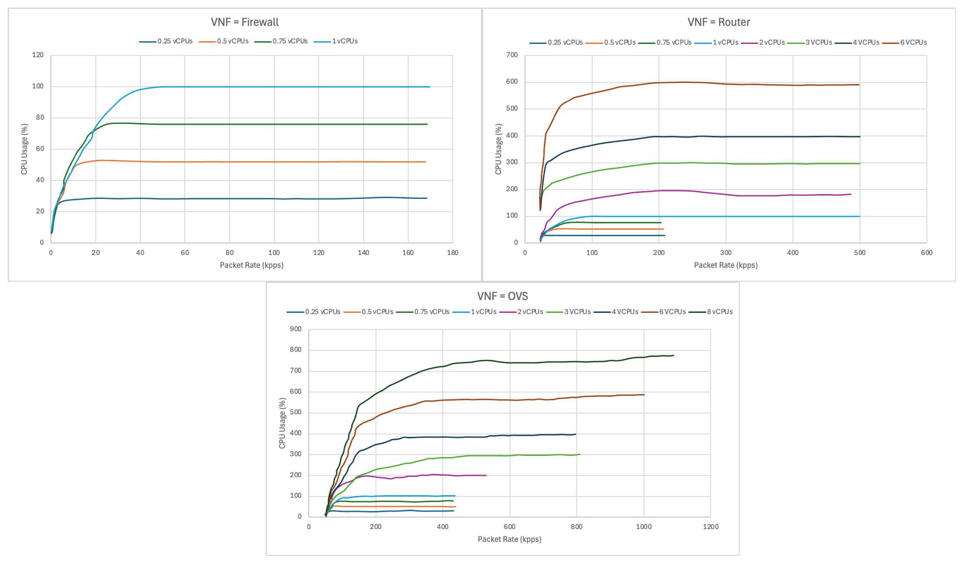
In this section, we show and compare different ML-based performance models that correlate the resource requirements of the VNF with the workload demand. The regression models considered in this work are those enumerated in Section 3.2, and the datasets used in these experiments are based on the performance profiling data obtained by [12] for three different VNFs commonly used in edge/5G-based IoT infrastructures (firewall, router, and OVS), as shown in Figure 2. These profiling data show the relationship between the input packet rate (in kpps) and CPU usage percentage for various hardware configurations (vCPUs) of the VNFs.

As mentioned in Section 3.3, to improve the performance of the different regression models, we implement a hyperparameter tuning based on a grid search combined with the k-fold cross-validation technique, as done in [9], using the RMSE as accuracy metric for selecting the best hyperparameter combination. The hyperparameter combinations used in these experiments, which are shown in

Table 2. Hyperparameter combinations used for grid search in regression models.

Model	Abbreviation	Hyperparameter Combinations
Linear Regression	Linear	No parameters
Ridge Regression	Ridge	alpha: [0.1, 1, 10]
Support Vector Regression	SVR	kernel: [’linear’, ’poly’, ’rbf’]
		C: [1, 10, 100]
		epsilon: [0.001, 0.01, 0.1]
Random Forest	Forest	n_estimators: [10, 100, 200]
Gradient Boosting Regression	Boost	learning_rate: [0.1, 0.15, 0.2, 0.25, 0.3]
		vn_estimators: [50, 100, 200, 300]
Multi-layer Perceptron regression	MLP	max_iter: [10,000]
		hidden_layer_sizes: [(50,), (100,), (200,)]
		alpha: [0.001, 0.0001, 0.00001]
		learning_rate_init: [0.01, 0.001, 0.0001]
		tol: [0.001, 0.0001]
Stochastic Gradient Descent regression	SDG	alpha: [0.0001, 0.001, 0.01, 1]
		epsilon: [0.01, 0.01, 0.1]
Gaussian regression	Gauss	alpha: [0.0001, 0.001, 0.01, 0.1, 1, 3, 5, 10]
		n_restarts_optimizer: [0, 2, 4, 6, 8]
K-Nearest Neighbors regression	KNN	n_neighbors: [2, 3, 4, 5, 6]
		weights: [’uniform’, ’distance’]
		algorithm: [’auto’, ’ball_tree’, ’kd_tree’, ’brute’]
		p: [1, 2]

, were determined through extensive offline experiments. In these experiments, we systematically explored variations in the hyperparameters to identify which combinations had the most significant impact on the accuracy of the models, using the datasets in this study. This process allowed us to empirically select the optimal hyperparameter ranges, based on the observed effects on model performance, rather than relying solely on domain knowledge or preliminary assumptions.

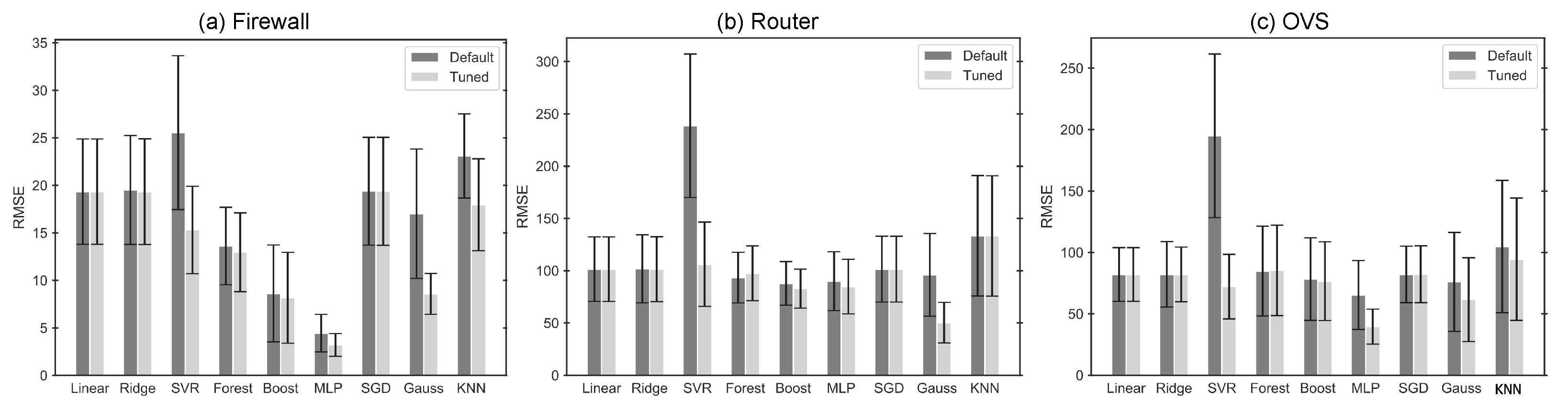
Figure 3 shows the RMSE of the various regression models for the three VNFs considered in this work. This figure also highlights the performance improvement that can be obtained on most models using hyperparameter tuning compared to the RMSE obtained with the default hyperparameters of each model.

Table 3. Training times for different regression models.

Training Time (s)				Inference Time (ms)
Model	Firewall	Router	OVS	Firewall	Router	OVS
Linear	0.01	0.01	0.01	0.22	0.22	0.22
Ridge	0.01	0.01	0.03	0.17	0.17	0.20
SVR	0.34	0.35	0.31	3.22	1.82	4.09
Forest	0.66	0.72	0.88	2.45	2.51	3.43
Boost	5.05	5.83	6.50	0.18	0.26	0.31
MLP	327.23	597.11	689.38	1.01	0.12	3.86
SGD	0.12	0.17	0.16	0.15	0.04	0.07
Gauss	0.40	0.61	61.15	42.82	49.11	62.07
KNN	0.32	0.34	0.35	0.29	0.35	1.13

shows the training times (with parameter tuning) and inference times for the different regression models evaluated. Linear, Ridge, SGD, KNN, and Gaussian models are the fastest to train, requiring less than one second (except for the Gaussian model applied to the OVS VNF, which takes up to 60 s). Boosting requires slightly higher training times, ranging from 5 to 7 s. In contrast, MLP exhibits the highest training cost, with values between 300 and 700 s. Regarding inference time, all models, except Gaussian, SVR, and Forest, provide predictions in less than one millisecond, with Gaussian being the slowest by a large margin, taking tens of milliseconds.

Table 4. Four best hyperparameter-tuned regression models for each VNF, sorted by RMSE.

VNF	4 Best Models (Sorted by RMSE)	Accuracy (RMSE)	Optimal Hyperparameters
Firewall	MLP	3.4	alpha: 0.0001; hidden_layer_sizes: (200,); learning_rate_init: 0.001; max_iter: 10,000; tol: 0.001
	Boost	8.3	learning_rate: 0.2; n_estimators: 200
	Gauss	8.6	alpha: 0.0001; n_restarts_optimizer: 0
	Forest	13.2	n_estimators: 100
Router	MLP	39.6	alpha: $1\times {10}^{-5}$; hidden_layer_sizes: (50,); learning_rate_init: 0.01; max_iter: 10,000; tol: 0.0001
	Gauss	61.6	alpha: 0.01; n_restarts_optimizer: 0
	SVR	72.2	C: 100; epsilon: 0.001; kernel: ’linear’
	Boost	76.6	learning_rate: 0.25; n_estimators: 200
OVS	Gauss	50.3	alpha: 0.0001; n_restarts_optimizer: 0
	Boost	82.9	learning_rate: 0.15; n_estimators: 200
	MLP	84.8	alpha: 0.0001; hidden_layer_sizes: (100,); learning_rate_init: 0.01; max_iter: 10,000; tol: 0.001
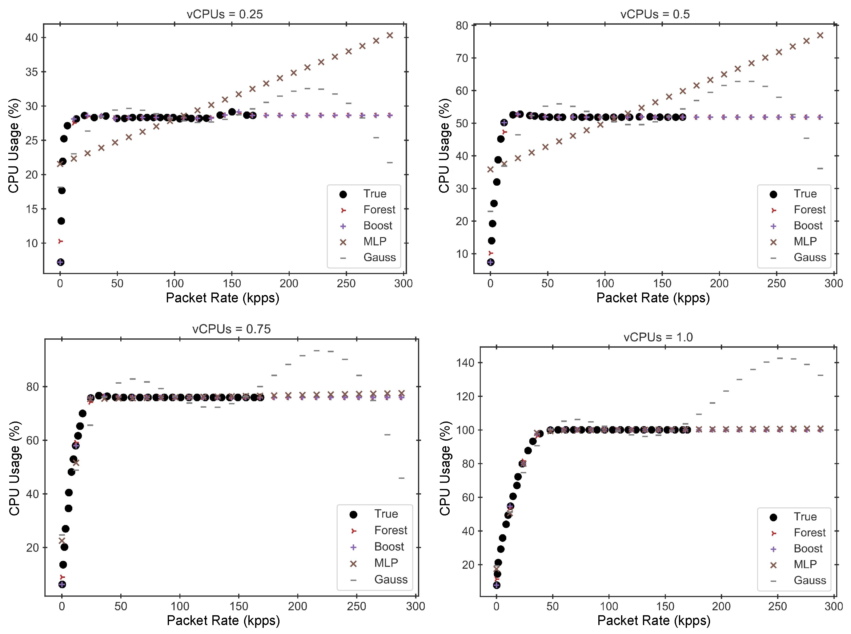
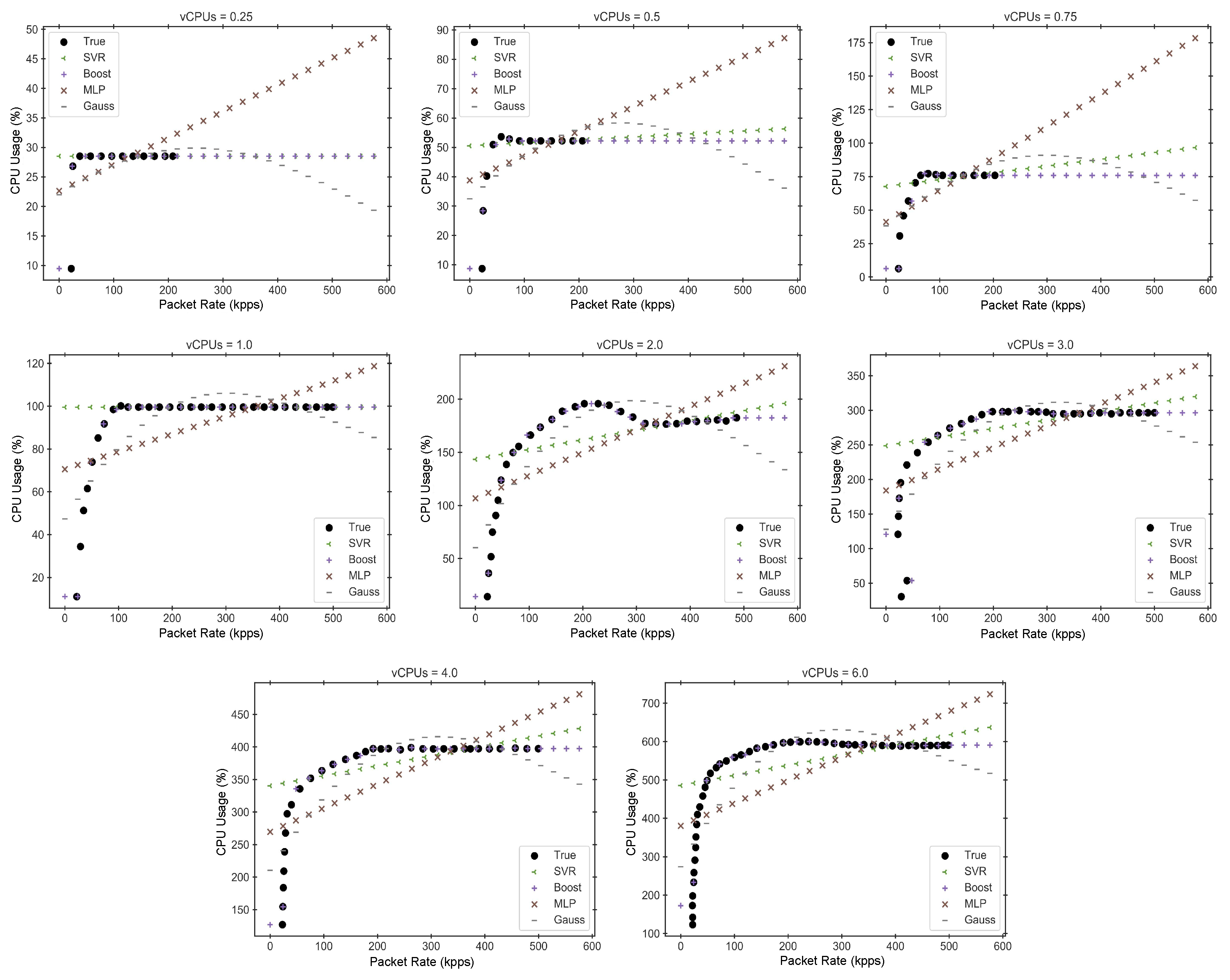
	Forest	97.5	n_estimators: 10

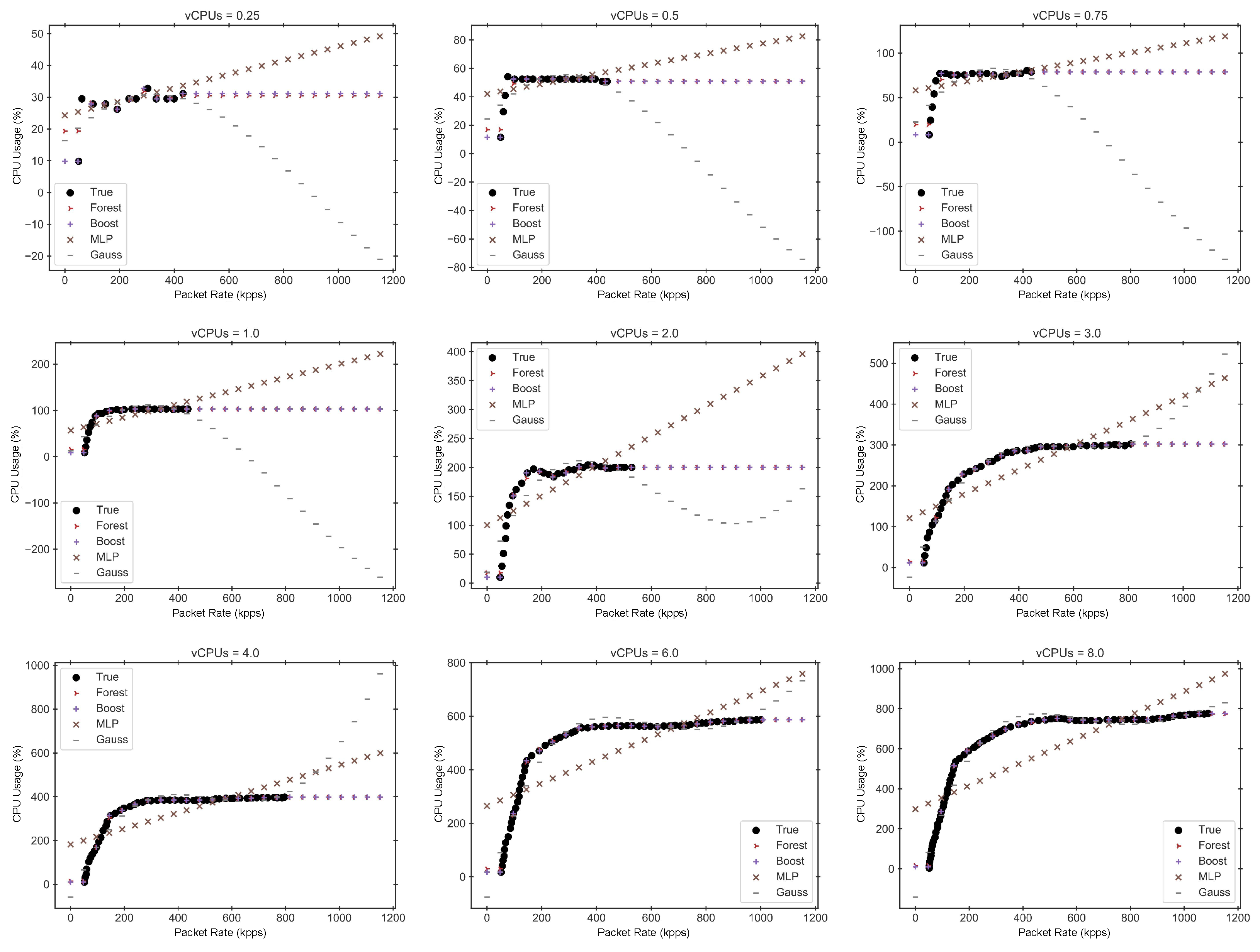
shows the four regression models that best behave for each VNF, along with the optimal hyperparameter combination of each model. Figure 4, Figure 5 and Figure 6 display the performance estimations obtained for these four best models, along with the true performance measurements of each VNF. To enhance the clarity of these figures, we have separated the data into multiple graphs, each corresponding to a different hardware configuration.

In light of the results presented in the previous graphs and tables, and based on the knowledge that the different VNFs exhibit an asymptotic behavior when the CPU reaches saturation, we conclude that Gradient Boosting Regression offers one of the best trade-offs between accuracy and both training and inference times across all cases. Therefore, this model will be used as the selected performance model for implementing the subsequent auto-scaling mechanisms.

6.2. Workload Forecasting Model Results

In this section, we show and compare different ML-based time series forecasting models to predict the workload demand for the VNFs. The forecasting models considered in this work are those enumerated in Section 4.2. The time-series datasets used in these experiments have been obtained from the traffic data repository maintained by the MAWI Working Group of the WIDE Project [22,71]. This dataset includes real daily traces at the transit link of WIDE to the upstream ISP, in operation since 2006. These traces contain anonymized traffic statistics from the WIDE backbone collected at two different frequencies (5 min and two hours). For our purposes, we have only used the aggregated traffic rate information, which is expressed in both bitrate (bps) and packet rate (pps). Specifically, in the subsequent experiments, we have chosen a one-month bihourly packet rate time series from 1 to 31 January 2024, as shown in Figure 7.

As mentioned in Section 4.3, to improve the performance of the different time series forecasting models, we implement a hyperparameter tuning based on a grid search, using the RMSE as accuracy metric for selecting the best hyperparameter combination. The combinations of hyperparameters used in these experiments are shown in

Table 5. Hyperparameter combinations used for grid search in time series forecasting models.

Time Series Forecasting Model	Hyperparameters Combinations
Regression	lags: [1, 2, 3, 6, 12, 18, 24, 36, 72]
	model: [LinearRegression(), Ridge(), BayesianRidge(), SGDRegressor(), Lasso(alpha=0.1)]
Random Forest	lags: [1, 2, 3, 6, 12, 24]
	n_estimators: [100, 200, 500]
	max_depth: [1, 10, 30]
XGBoost	lags: [1, 2, 3, 6, 12, 24, 36, 72]
TCN	input_chunk_length: [3, 6, 12, 24]
	kernel_size: [1, 2]
	dropout: [0.1, 0.4]
	num_layers: [1, 2, 3, 4]
	num_filters: [1, 3, 5]
	dilation_base: [2, 4]
	n_epochs: [100]
RNN_GRU	input_chunk_length: [2, 6, 12, 24]
	model: [“GRU”]
	hidden_dim: [3, 5, 10]
	n_rnn_layers: [1, 2, 4]
	n_epochs: [100]
RNN_LSTM	input_chunk_length: [2, 6, 12, 24]
	model: [“LSTM”]
	hidden_dim: [3, 5, 10]
	n_rnn_layers’: [1, 2, 4]
	n_epochs: [100]
Transformer	input_chunk_length: [2, 6, 12, 24]
	nhead: [2, 4, 8]
	num_encoder_layers: [2, 3, 4]
	num_decoder_layers: [2, 3, 4]
	dim_feedforward: [128, 512, 1024]
	n_epochs: 100

. As in the previous case, these combinations were determined through extensive offline experiments. The first two models (Regression and Random Forest) are non-probabilistic forecast models, while the last four models (XGBoost, TCN, RNN_GRU and RNN_LSTM) can implement probabilistic forecasts, based on quantiles.

Table 6. Training and prediction times for different time series forecasting models.

Model	Training Time (s)	Prediction Time (ms)
Regression	0.1	30.3
Random Forest	4.9	23.7
XGBoost	1.0	13.3
TCN	166.0	657.7
RNN_GRU	27.3	96.4
RNN_LSTM	27.4	30.4
Transformer	1651.7	1120.6

presents the training and prediction times for the different time series forecasting models. Regression is the fastest in terms of training time (0.1 s), followed by XGBoost (1.0 s) and Random Forest (4.9 s). RNN-based models (GRU and LSTM) show moderate training times (around 30 s). In contrast, TCN and Transformer models have the longest training times, approaching 3 and 30 min, respectively. Regarding prediction times, XGBoost is the fastest model (13.3 ms), while all other models have prediction times below 100 ms, except for TCN and Transformer, which require 0.66 and 1.65 s, respectively.

Table 7. Optimal hyperparameter and accuracy for different time series forecasting models.

Time Series Forecasting Model	Accuracy (RMSE)	Optimal Hyperparameters
Regression	54.5	lags: 18; model: SGDRegressor()
Random Forest	29.2	lags: 12; n_estimators: 500; max_depth: 30
XGBoost	38.2	lags: 1
TCN	68.5	input_chunk_length: 24; kernel_size: 1; dropout: 0.1; num_layers: 1; num_filters: 1; dilation_base: 4; n_epochs: 100
RNN_GRU	104.6	input_chunk_length: 24; model: “GRU”; hidden_dim: 3; n_rnn_layers: 2; n_epochs: 100
RNN_LSTM	129.0	input_chunk_length: 24; model: “LSTM”; hidden_dim: 3; n_rnn_layers: 2; n_epochs: 100
Transformer	48.3	input_chunk_length: 2; nhead: 8, num_encoder_layers: 2, num_decoder_layers: 4, dim_feedforward: 1024, n_epochs: 100

shows the optimal hyperparameter combination of each model and the corresponding model accuracy (RMSE). As we can observe, Random Forest and XGBoost are the models that best behave in terms of the accuracy of the prediction. Additionally, they also exhibit some of the lowest training and prediction times among all the models. The Transformer-based model also achieves good accuracy, but it requires significantly higher training and prediction times. Figure 8 displays the time series forecasting results obtained for all six forecasting models. For probabilistic models, the prediction intervals shown in the figure are based on the 5th and 95th percentiles. The predictions are made over the last n values of the time series (with n = 100 in our experiments) to allow us to compare the actual and predicted values. However, we do not predict all n values in a single step. Instead, we use the historical forecast function of the Darts library with a forecast horizon of 1. This function repeatedly builds a training set, expanding from the beginning of the series up to the point just before the current prediction, and emits a forecast of length equal to the forecast horizon.

6.3. Horizontal Auto-Scaling Results

In this subsection, we analyze the results of the horizontal auto-scaling mechanisms. For this purpose, we have selected the pre-trained performance model based on Gradient Boosting Regression for the three VNFs considered: Firewall, Router, and OVS. Additionally, for workload prediction, we have considered two different pre-trained forecasting models: the non-probabilistic Random Forest model and the probabilistic XGBoost model, with prediction intervals based on the 5th and 95th percentiles. According to the horizontal auto-scaling mechanism explained in Section 5.1, in addition to selecting the performance and forecasting models, it is necessary to choose a value for the CPU utilization threshold and define the hardware configuration of the virtual instance types used for the deployment, expressed in terms of the number of vCPUs. In the following experiments, we have chosen a fixed value of 95% for the CPU utilization threshold, meaning the CPU usage of the allocated virtual instances cannot exceed 95% of the available vCPUs. On the other hand, we have selected a limited subset of hardware configurations for the virtual instance types, tailored to the particularities of each of the VNFs considered. In particular, we have considered the hardware configurations shown in

Table 8. Hardware configurations of different VM instance types used in the experiments.

VNF	Hardware Configurations for VM Instances
	0.5 vCPUs
Firewall	0.75 vCPUs
	1.0 vCPUs
	0.5 vCPUs
Router	1.0 vCPUs
	2.0 vCPUs
	1.0 vCPUs
OVS	2.0 vCPUs
	4.0 vCPUs

.

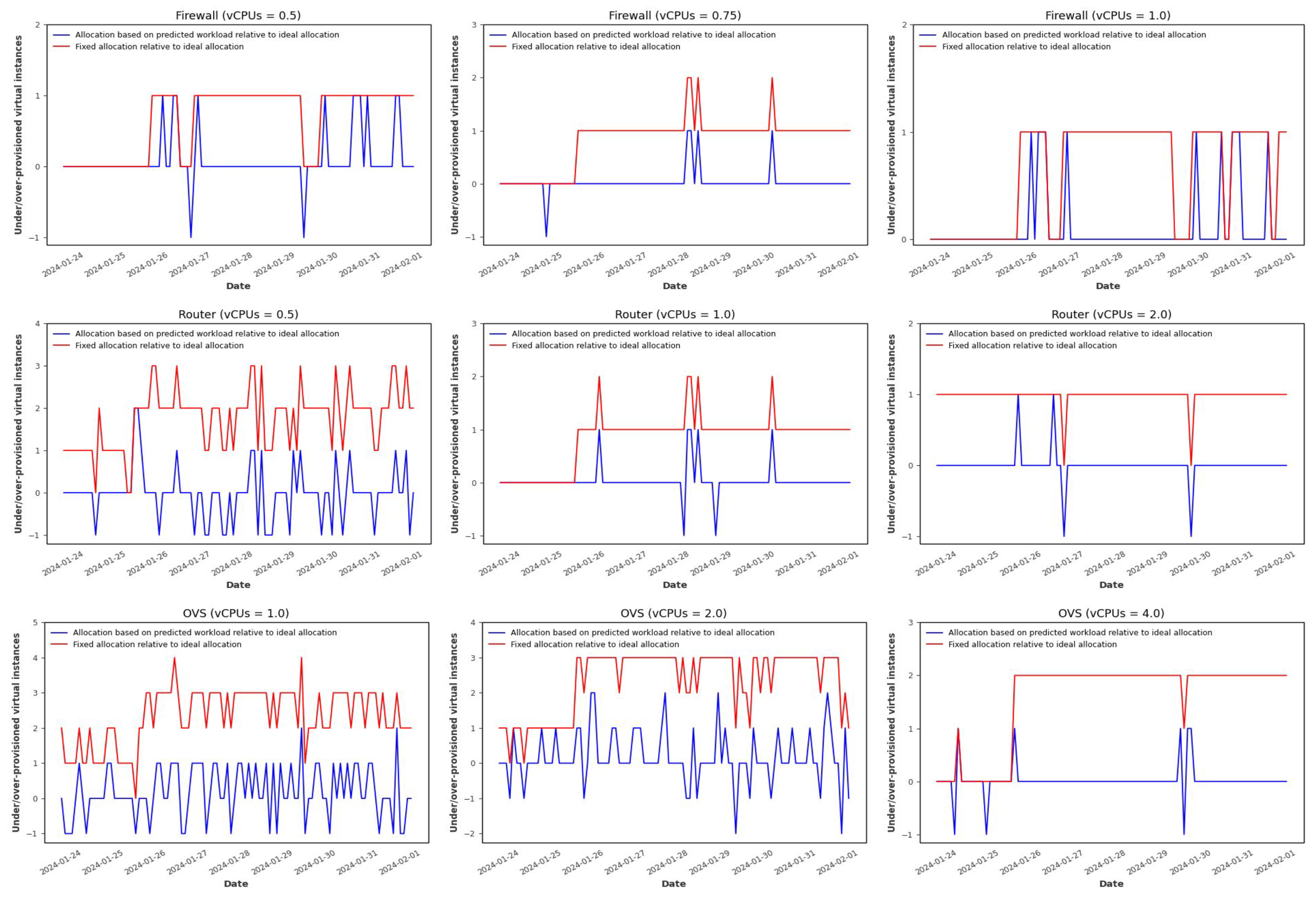
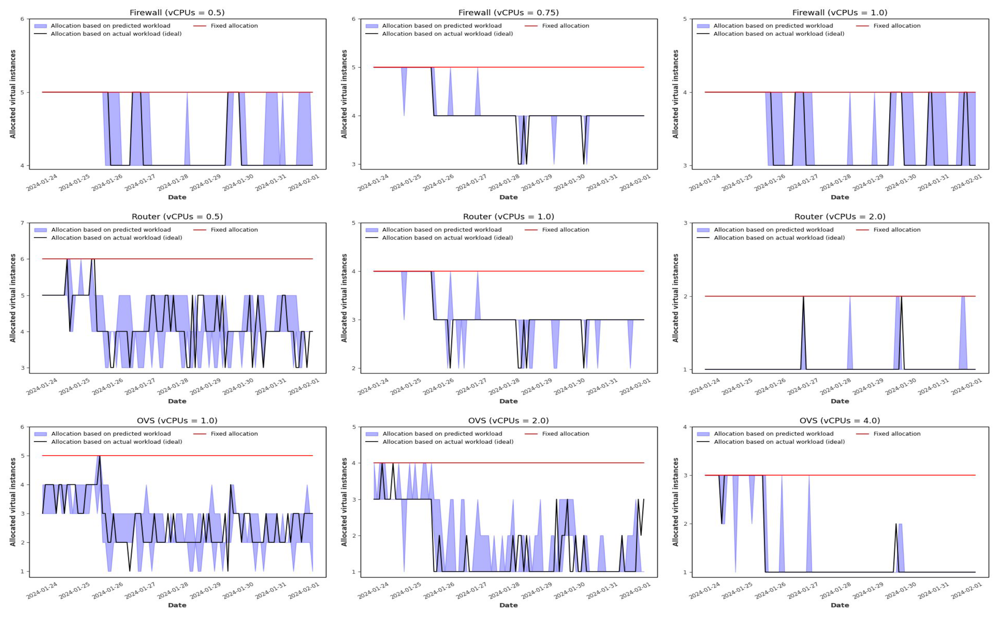
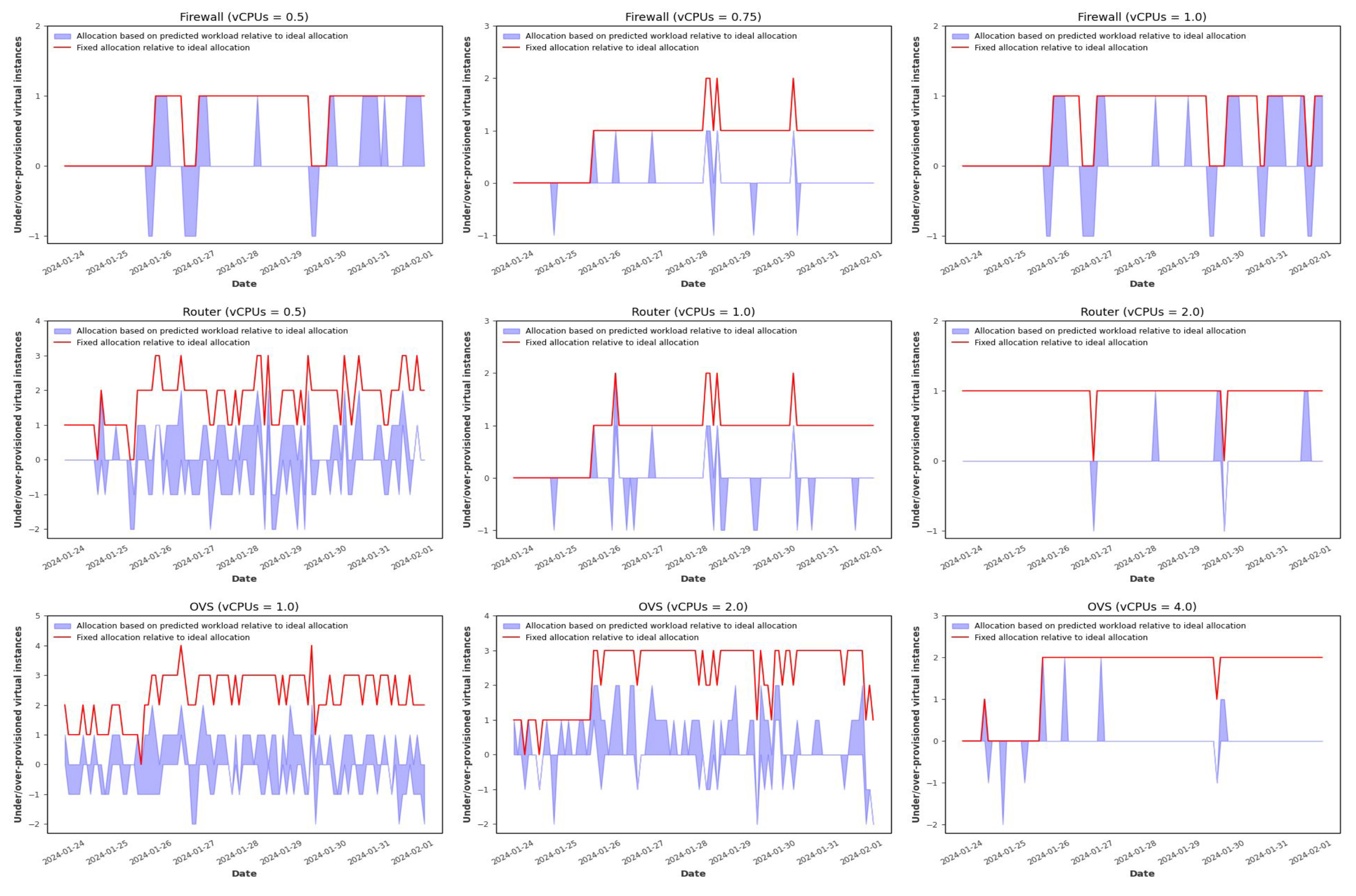
Figure 9 displays the allocation results with horizontal auto-scaling for the three VNFs and different hardware configurations when using the Random Forest-based forecasting model. These graphs compare three different allocation strategies: the horizontally auto-scaled allocation based on predicted workload (using the Random Forest model), the horizontally auto-scaled allocation based on the actual workload (ideal case), and a fixed allocation mechanism that uses a constant amount of resources to satisfy the maximum workload demand and avoid under-provisioning at any time interval. It is important to note that, although ideal, allocation based on the actual workload is unfeasible in a realistic scenario since the actual workload for the next scheduling interval cannot be known in advance. However, in our case, as we are working with historical forecasts, this information is available and very valuable for assessing the effectiveness of the proposed predictive auto-scaling mechanisms. As we can observe, the fixed allocation results in significant over-provisioning compared to the ideal allocation, while the allocation based on predicted workload better accommodates fluctuations in workload. This is clearly illustrated in Figure 10 and Figure 11, which show the over- and under-provisioning of resources for the fixed and predicted workload-based allocations, measured relative to the ideal case. 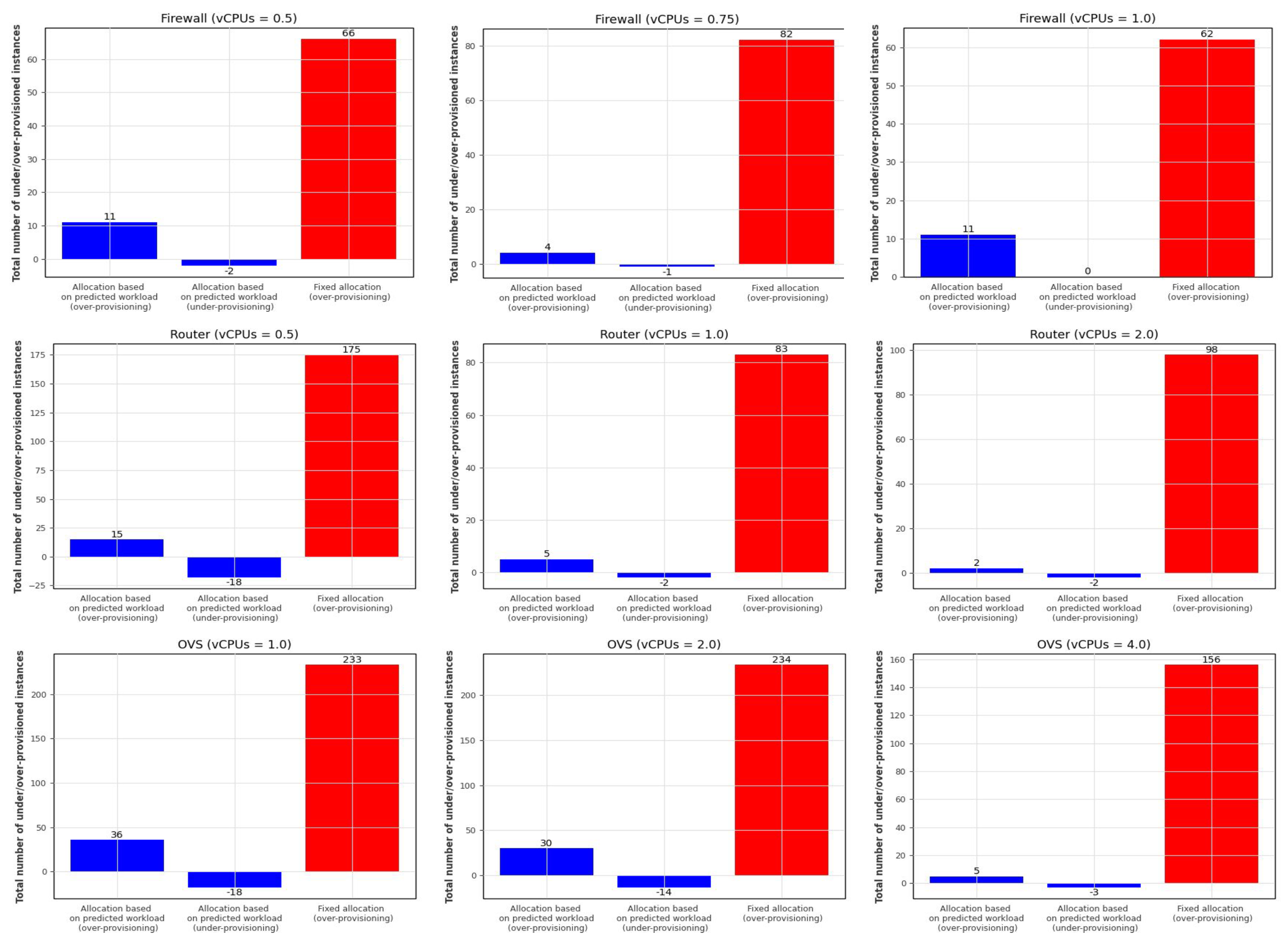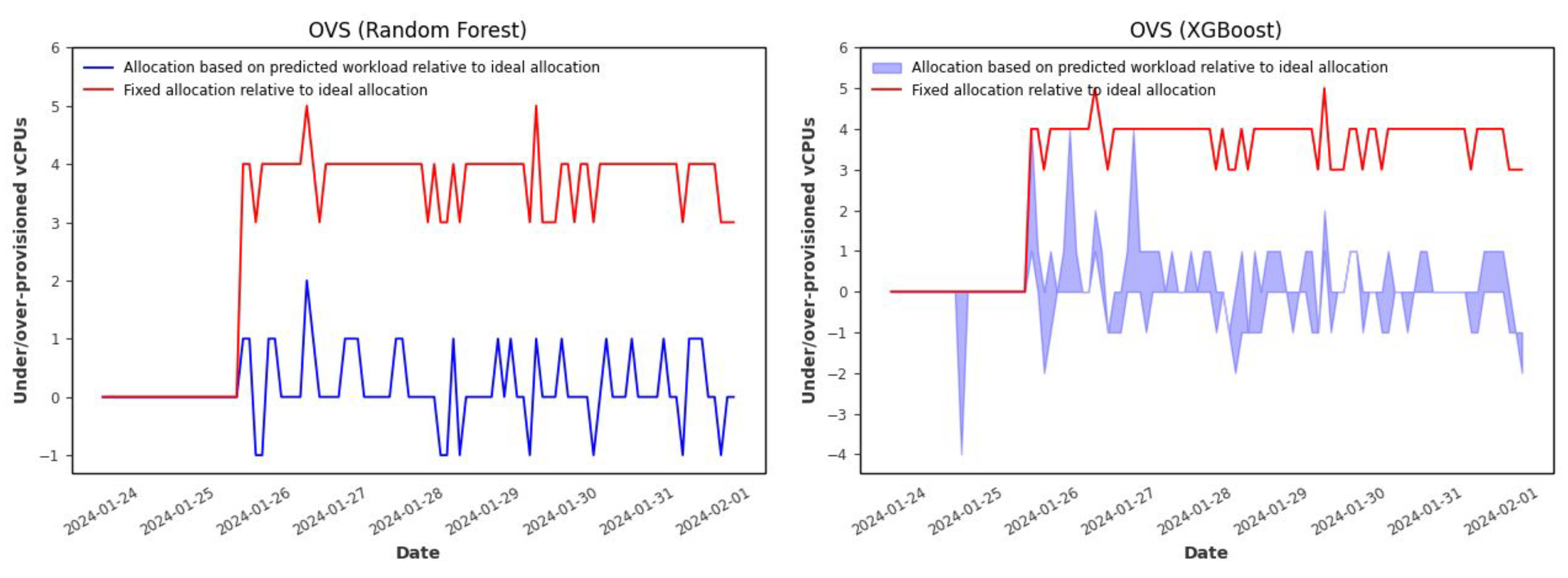Figure 10 displays the over- and under-provisioning at each time step, while Figure 11 presents the total number of over- and under-provisioned resources in each case. In this Figure, the two left bars (blue) represent the total number of over- and under-provisioned resources of the allocation based on predicted workload relative to the ideal allocation and the right bar (red) represents the total number of over-provisioned resources of the fixed allocation relative to the ideal allocation. As we can see, although the fixed allocation never incurs under-provisioning, its over-allocation is much more pronounced than that of the predicted workload-based allocation.

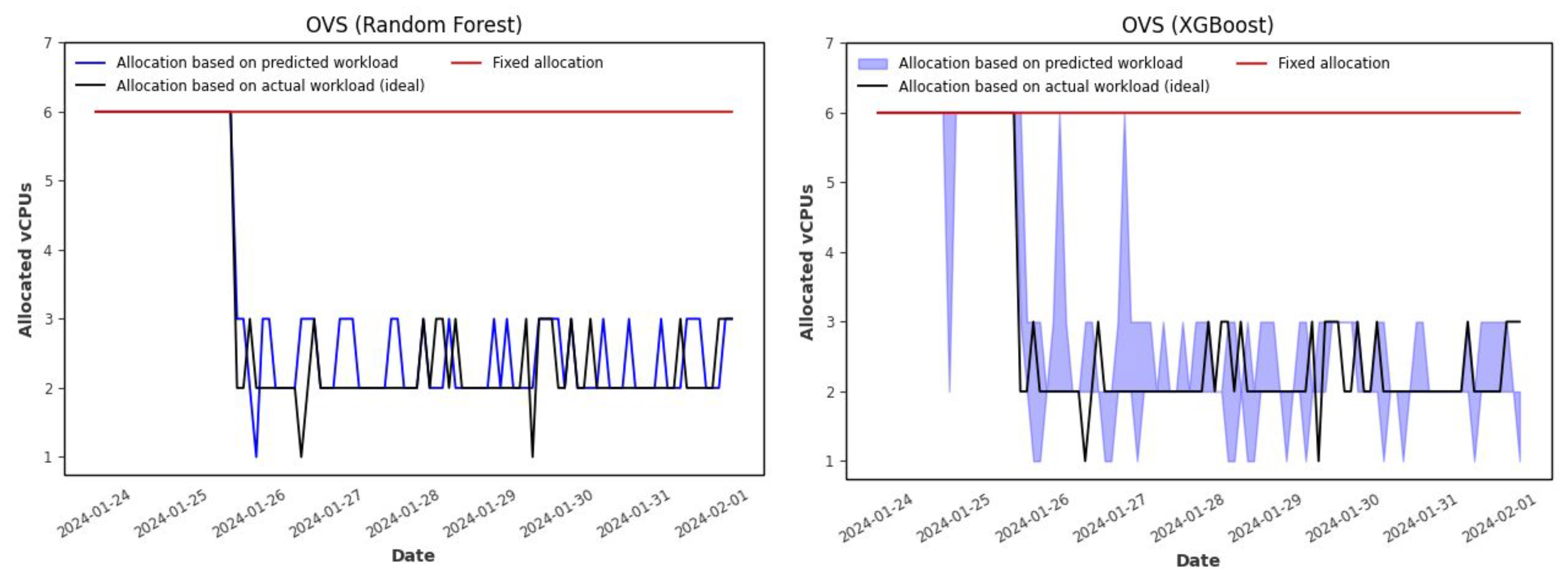
Next, we analyze the horizontal auto-scaling results obtained with the XGBoost forecasting model. Figure 12 compares the horizontally auto-scaled allocation based on predicted workload (using the XGBoost model), the horizontally auto-scaled allocation based on the actual workload (ideal case), and the fixed allocation mechanism. As we can observe, with the allocation based on the XGBoost forecasting model, instead of having a single allocation value for each time step, we can have a range of values corresponding to the lower and upper bounds of the workload prediction intervals (5th and 95th percentiles, respectively). As in the previous case, compared to the ideal case (allocation based on actual workload), the fixed allocation results in significant over-provisioning, while the allocation based on predicted workload better accommodates fluctuations in workload. This is clearly illustrated in Figure 13 and Figure 14. Figure 13 displays, for each time step, the number of over- or under-provisioned resources of the fixed and predicted workload-based allocations relative to the ideal allocation. In Figure 14, the two bars on the left and the two bars in the middle represent the total number of over- and under-provisioned resources of the allocation based on the upper and the lower bounds of the workload prediction interval, respectively, relative to the ideal allocation. The right bar (red) represents the total number of over-provisioned resources of the fixed allocation relative to the ideal allocation.

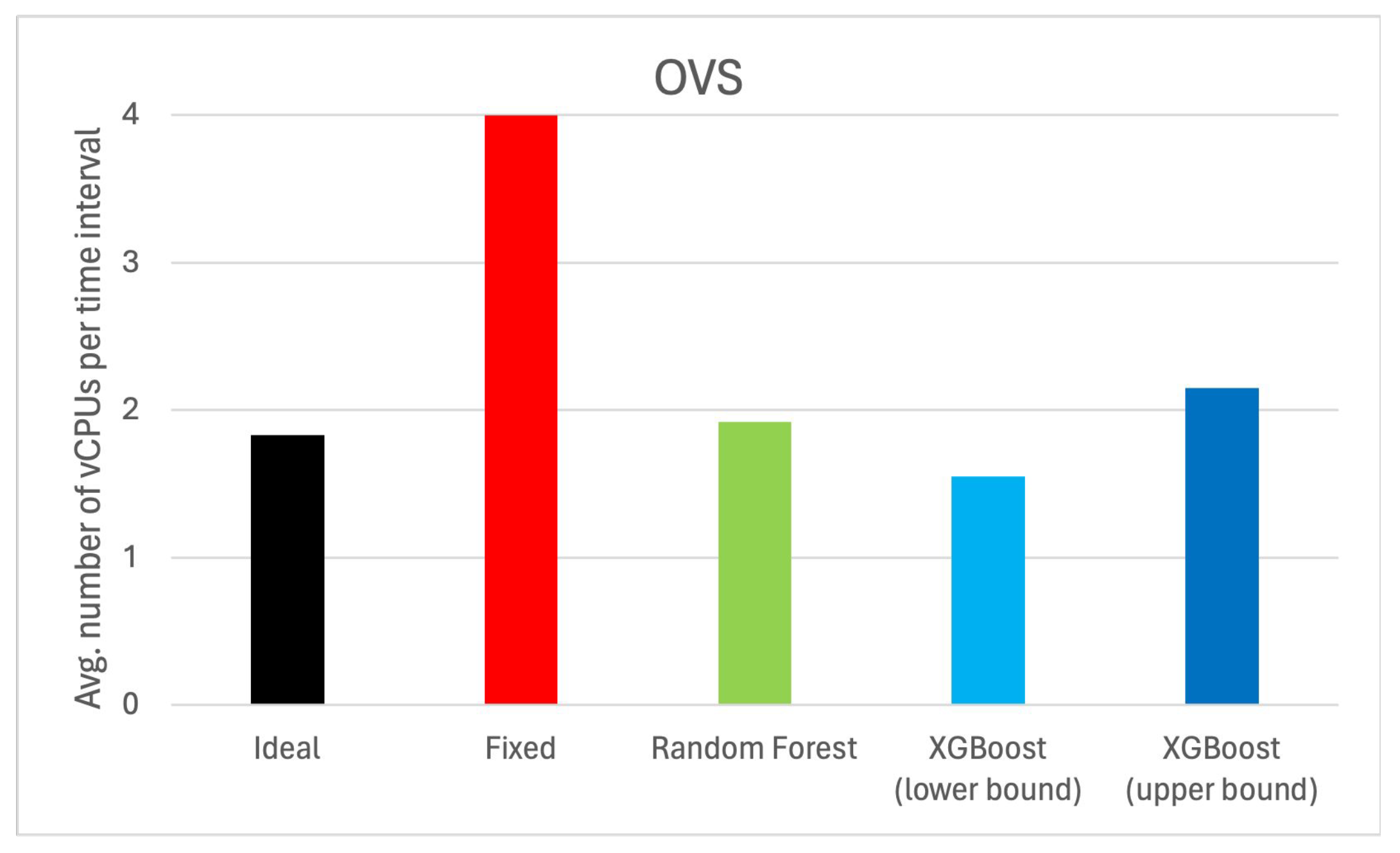
Finally, Figure 15 compares the average number of vCPUs allocated per time step for each combination of VNF and hardware configuration, and different allocation mechanisms (ideal, fixed, based on Random Forest prediction, and based on the lower and upper bound intervals of XGBoost prediction). As we can see, although the allocation mechanisms based on workload prediction can result in a slightly higher number of vCPUs allocated per time interval, the resource savings compared to fixed allocation are very significant, ranging between 9% and 57%.

Regarding all the previous results, and considering that under-provisioning should be avoided as far as possible due to the risk of service quality degradation, data loss, or even service failures, and that over-provisioning has its own significant drawbacks, such as unnecessary resource wastage, higher power consumption, and increased costs, the optimal trade-off between under-provisioning and over-provisioning is achieved by using the allocation based on the upper bound prediction interval of the XGBoost model.

6.4. Vertical Auto-Scaling Results

In this subsection, we analyze the results of the vertical auto-scaling mechanisms. As in the previous case, we have selected the pre-trained performance model based on Gradient Boosting Regression, and two different pre-trained forecasting models for workload prediction: the non-probabilistic Random Forest model and the probabilistic XGBoost model, with prediction intervals based on the 5th and 95th percentiles. The experiments with vertical auto-scaling are conducted using a single VNF: the OVF. For these experiments, we consider a CPU utilization threshold of 95% and a set of virtual instance types with different hardware configurations, sorted by the number of vCPUs. Specifically, we consider the following hardware configurations: 1.0, 2.0, 3.0, 4.0, 6.0 and 8.0 vCPUs. Figure 16 presents the allocation results of vertical auto-scaling based on predicted workload using Random Forest and XGBoost models, compared to ideal vertical auto-scaling allocation based on actual workload and fixed allocation, which uses a constant number of vCPUs to meet the maximum workload demand and avoid under-provisioning. As shown, the fixed allocation leads to significantly higher over-provisioning of vCPUs compared to the allocation based on predicted workload, which more effectively adapts to variable workloads. This is more clearly illustrated in Figure 17 and Figure 18, which display the number of over-provisioned vCPUs per time step and in total, respectively, resulting from the predicted workload-based allocation and fixed allocation, relative to the ideal allocation. Finally, Figure 19 compares the average number of vCPUs allocated per time step using vertical auto-scaling with different allocation mechanisms (ideal, fixed, based on Random Forest prediction, and based on the lower and upper bound intervals of XGBoost prediction). As we can see, the average number of vCPUs allocated for mechanisms based on workload prediction is slightly higher than the ideal case, but much lower than that obtained by the fixed allocation, resulting in resource savings ranging between 46% and 61%. Similar to the case of horizontal auto-scaling, the solution that minimizes under-provisioning while maintaining reasonable values of over-provisioning is the allocation based on the upper bound prediction interval of the XGBoost model.

While the proposed models show acceptable results in terms of under-provisioning, prediction errors may still lead to an insufficient allocation of resources, whether in vertical or horizontal auto-scaling, which could compromise the system’s ability to meet workload demands. To mitigate this issue, hybrid auto-scaling mechanisms that combine predictive strategies with reactive components represent a promising direction. By monitoring runtime performance and triggering corrective actions when necessary, these hybrid approaches can offer greater robustness and adaptability. Recent studies have shown the potential of such methods to improve the reliability and responsiveness of auto-scaling frameworks under dynamic conditions [72,73]. Integrating these techniques into our framework will be considered in future work.

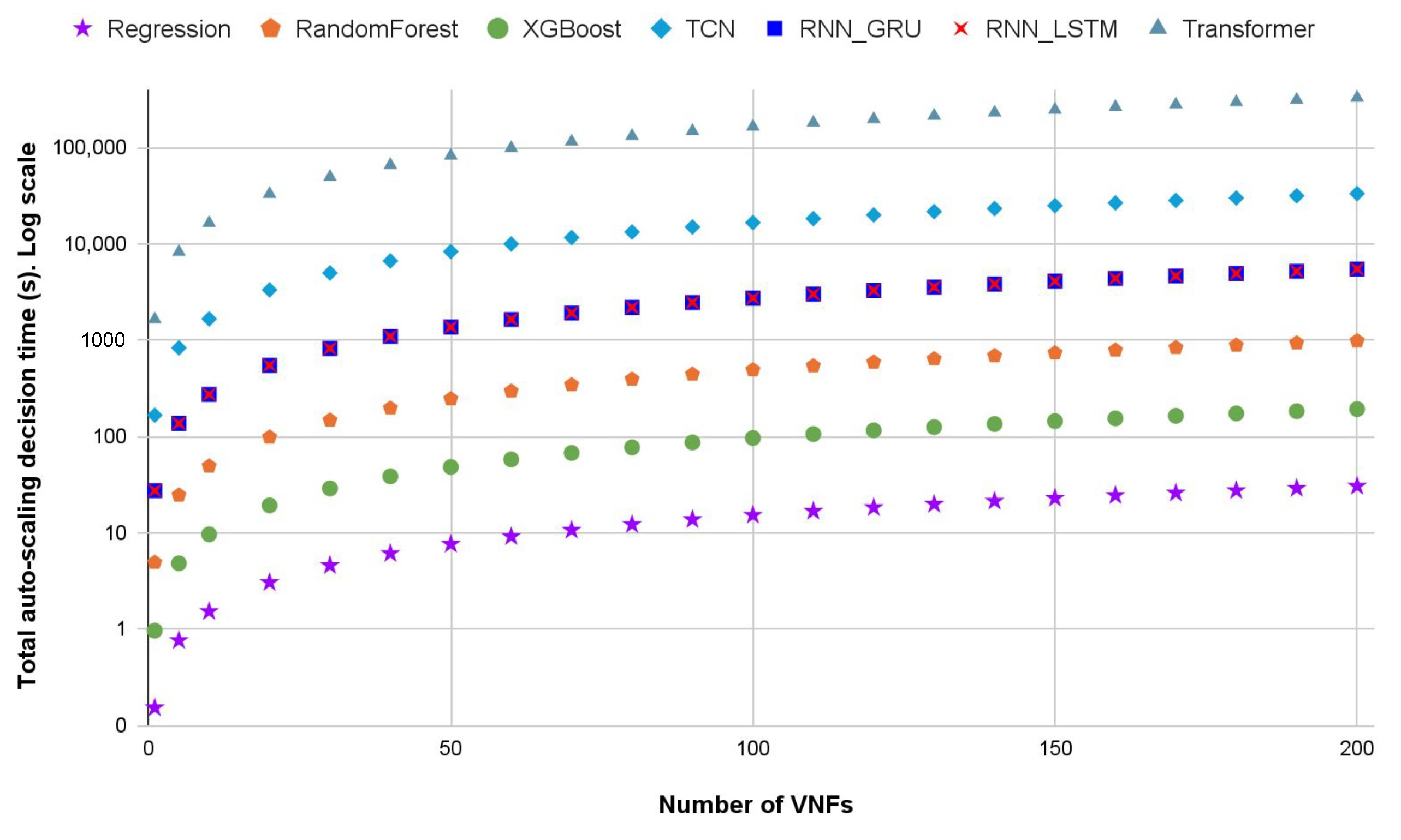
6.5. Scalability Analysis of the Auto-Scaling Mechanisms

To assess the scalability of the proposed auto-scaling framework, we conducted a performance analysis focused on the end-to-end decision-making time required at each scheduling interval. This time includes all the components involved in executing the auto-scaling mechanism for a variable number of VNFs.

Specifically, for each VNF, the following steps are performed at every scheduling interval:

• Re-training of the workload forecasting model using the most recent workload data;
• Prediction of the VNF workload for the upcoming interval using the updated time series model;
• Inference of the required resources for the VNF using the performance model;
• Execution of the auto-scaling algorithm to determine the final allocation.

We measured the total execution time required to perform these steps across an increasing number of VNFs, ranging from 1 to 200. The re-training time reflects the overhead introduced by periodic model updates in response to dynamic workload patterns, which is particularly relevant in edge environments where computational resources are limited. These steps are common to both horizontal and vertical auto-scaling mechanisms, and the decision-making time has been observed to be similar in both cases.

Figure 20 illustrates the total decision-making time of the auto-scaling mechanism as a function of the number of VNFs for each of the evaluated forecasting models. For instance, for 200 VNFs, the auto-scaling algorithm may require approximately 3 min to complete the decision-making process when using the XGBoost model, while the Random Forest model may take around 16 min. On the other hand, using RNN-based models such as GRU and LSTM, the decision-making time increases significantly, reaching up to 1.5 h. Models based on TCN and Transformer architectures exhibit even higher computational costs, requiring several hours to complete the decision for 200 VNFs.

These execution times could be substantially reduced by leveraging high-performance training platforms equipped with GPUs, or other specialized hardware. However, such hardware is not always available in Edge-IoT-5G environments, which are often characterised by modest computing capabilities and stringent energy consumption constraints.

As expected, the execution time grows approximately linearly with the number of VNFs. Nevertheless, the increase remains within acceptable limits when using lightweight models such as XGBoost, with total decision times remaining well below the typical length of a scheduling interval (e.g., 5 min). This suggests that the framework can scale to medium-sized edge deployments without violating real-time constraints, provided that suitable forecasting models are selected. These results confirm that the proposed approach is computationally feasible and scalable, supporting its practical deployment in real-world edge-5G-IoT scenarios.

7. Conclusions and Future Work

This paper presents a functional framework for AI-driven resource allocation and auto-scaling of VNFs in edge/5G-enabled IoT environments, relying on established machine learning techniques rather than focusing on the development of new ones. Our approach combines performance profiling, ML-based performance modeling, and workload forecasting to implement predictive auto-scaling mechanisms. We illustrate that accurate predictions can be obtained by employing simple yet effective ML models, such as random forest or gradient boosting, making our approach suitable for real-world environments that require frequent model retraining and estimations, allowing rapid auto-scaling decision-making. The different experiments achieved, based on real traffic data, validate our framework’s capacity to dynamically adjust resources in response to traffic demands while reducing both over- and under-provisioning.

Future research directions include extending the framework to support a broader range of VNFs and diverse SFC scenarios, as well as evaluating new machine learning and deep learning mechanisms for performance modeling and time series forecasting. We also plan to explore more advanced hyperparameter tuning techniques to enhance the efficiency of the auto-scaling mechanisms. While grid search was employed in this study for its simplicity and ease of implementation, it can become computationally expensive, particularly as the hyperparameter space grows. To address this limitation, we plan to investigate Bayesian optimization, which uses probabilistic models to intelligently explore the hyperparameter space and prioritize the most promising configurations. Additionally, we will consider evolutionary algorithms, such as genetic algorithms, which are well-suited for efficiently searching large and complex parameter spaces.

Furthermore, we plan to integrate our auto-scaling mechanisms with intelligent placement strategies to enable the optimal mapping of VNFs to physical servers across geographically distributed 5G edge locations, considering various optimization criteria such as energy efficiency and overall Service Function Chain (SFC) latency. For this research, we intend to explore a combination of classical optimization techniques, such as integer linear programming, and intelligent techniques, particularly those based on reinforcement learning (RL) and deep reinforcement learning (DRL). RL and DRL offer several advantages for this type of problem, as they enable the system to learn optimal placement strategies through interaction with the environment, rather than relying on predefined models or exhaustive search. These approaches can dynamically adapt to changing network conditions, workload fluctuations, and evolving user demands, making them particularly well-suited for the highly dynamic and distributed nature of 5G edge networks.

In addition, future work will explore more challenging and extreme network scenarios, such as traffic spikes or DDoS (Distributed Denial of Service) attacks. These types of situations pose unique challenges for auto-scaling mechanisms and resource allocation strategies, as they can cause sudden and significant shifts in traffic patterns and network behavior. By studying these scenarios, we aim to improve the resilience and adaptability of our framework in handling abnormal conditions, ensuring that the system can effectively manage the increased load and mitigate the potential impact of such events on the overall network performance.

Finally, the development of hybrid auto-scaling mechanisms that combine the predictive strategies proposed in this study with reactive approaches is also contemplated as future work, in order to correct the potential effects of prediction errors that may lead to insufficient resource provisioning.