Efficient Interference Detection for Satellite Communications Based on Non-Uniform Adaptive Segmentation

Abstract

Interference detection is one of the key technologies used in satellite communication systems to cope with complex electromagnetic environments. To accommodate the power consumption and resource-constrained application scenarios of communication satellite payloads, this paper proposes an efficient differential amplitude interference detection algorithm based on non-uniform adaptive segmentation, building upon the classical forward consecutive mean excision (FCME) algorithm in the field. The proposed algorithm replaces the traditional point-based iterative approach with a segment-based iterative strategy and employs a non-uniform adaptive segmentation scheme to achieve rapid and efficient iterative updates of detection thresholds. This significantly reduces the complexity of the whole interference detection process. Simulation experiments were conducted on different types of interference signals, and the results verified the effectiveness of the proposed algorithm.

1. Introduction

With the increasing complexity of the space electromagnetic environment and the growing openness of satellite communication links, satellite communication systems are highly susceptible to various intentional and unintentional electromagnetic interference, which can severely degrade communication performance. Therefore, the adoption of effective communication anti-jamming technologies is of great importance. Interference detection aims to analyze the location, power, and other parameters of interference within the received signal, providing essential foundations for the formulation and implementation of subsequent anti-jamming strategies. However, most existing interference detection algorithms exhibit high complexity and substantial computational requirements; while the computational resources of satellite payloads are highly valuable, their processing capability and power consumption are strictly constrained. Therefore, from the perspective of reducing system resource consumption, research on lightweight and efficient interference detection algorithms not only provides sufficient prior information for anti-jamming measures, but also enhances the anti-jamming capability of satellite communication systems, thereby improving overall system reliability.

At present, research on interference detection algorithms by scholars in the field is relatively extensive and primarily categorized into two major types: binary interference detection algorithms and frequency-domain interference detection algorithms. Binary interference detection algorithms include classical methods, such as energy detection algorithm [1,2], cyclic autocorrelation detection algorithm [3,4,5], matched filtering detection algorithm [6,7,8], etc. However, these methods have inherent limitations, as they can only determine the presence of interference but cannot provide precise spectral location, power, and other key parameters of the interference signal. This limitation restricts their applicability in refined interference analysis and the formulation of anti-jamming strategies.

To overcome this technical bottleneck, frequency-domain interference detection algorithms have been extensively studied and applied. P. Henttu et al. proposed the consecutive mean excision (CME) algorithm [9], which employs iterations to classify all samples into a noise set and an interference set [10]. However, since this method initially assumes that all samples belong to the noise set, it is not suitable for broadband interference detection. Johanna Vartiainen improved the CME algorithm and proposed the forward consecutive mean excision (FCME) algorithm [11], which optimizes the initial threshold calculation by sorting the amplitude of all samples in ascending order (taking the first 10% of the samples as noise set at first). However, the drawback of this algorithm is its high complexity [12]. To further enhance interference signal detection accuracy, reference [13] proposed the localization algorithm based on double-thresholding (LAD), which sets high and low thresholds to respectively prevent misclassification and missed detections of interference signals, thereby reducing the false alarm probability. Building upon this, reference [14] proposed the localization algorithm based on double-thresholding adjacent cluster combining (LAD-ACC), which addresses the signal segmentation problem by merging adjacent signal clusters. Additionally, reference [15] builds upon the double-threshold FCME algorithm by incorporating a predefined intermediate threshold to process the spectrum of the received signal, achieving effective detection of narrowband interference under high signal-to-noise ratio conditions.

In recent years, deep learning has been extensively applied in the field of broadband interference signal detection. The study in [16] proposed a one-dimensional fully convolutional network (FCN), which was validated on real satellite signal data, demonstrating its effectiveness. In [17], an intelligent broadband detection algorithm based on an improved You Only Look Once v3 (YOLOv3) object detection network was proposed. This algorithm detects non-cooperative signals from broadband time-frequency spectrograms, achieving high detection accuracy. However, these methods rely on large-scale datasets for neural network training, which results in a high computational load and may not be able to adapt to the resource-constrained environment of satellite payloads.

It is worth noting that, in addition to conventional interference detection and suppression strategies, for the interference among multiple users within the network, recent studies have explored treating interference structures as tunable design variables to enhance system sum rate and spectral efficiency. For example, Bing. L et al. [18] proposed a scheme based on multiantenna nonorthogonal multiple access (mNOMA) technique that exploits interference aggregation patterns under overloaded access conditions to construct power and modulation structures, achieving the quality of service (QoS) guarantees and improved system sum rate, using only partial channel state information (CSI). Although such approaches differ from the interference detection focus of this work, they reflect a new research trend toward treating interference as a potential resource rather than merely a limitation.

In non-interference signals, the noise spectrum remains relatively flat, resulting in small amplitude differences between the front and back of the spectrum. In contrast, interference-containing signals exhibit significant amplitude fluctuations in the spectrum. Based on this spectral characteristic, F. Li et al. [19] proposed a differential amplitude-based FCME algorithm, which replaces the traditional sorting process with a segmented differential approach. This method enables rapid estimation of background noise and calculation of the initial threshold while maintaining a similar detection probability and improving computational efficiency [20]. However, the fixed segmentation parameters limit the algorithm’s adaptability, and there is still room for further optimization to enhance algorithm efficiency and parameter adaptability.

Inspired by the segmented differential approach in F. Li et al.’s differential amplitude-based FCME algorithm [19], and addressing the shortcomings of existing algorithms, this paper proposes an efficient differential amplitude interference detection algorithm based on non-uniform adaptive segmentation. The proposed algorithm divides the samples into segments in a non-uniform, adaptive, and dynamic manner to optimize the calculation of the initial threshold. Additionally, it effectively utilizes the segment-based strategy to replace the traditional point-based iterations with segment-based iterations. Through simulation verification, the proposed algorithm significantly improves the computational efficiency of interference detection while ensuring detection performance.

2. Interference Signal Models

• Single-Tone Interference

Single-tone interference is one of the most fundamental forms of suppression jamming. It modulates a waveform of a single frequency onto a specific carrier frequency, resulting in concentrated high energy at that frequency while leaving other frequencies unaffected. This type of interference is typically used when the communication frequency band is known in advance, serving a targeted suppression function. In the time domain, it appears as a sinusoidal waveform, while in the frequency domain, it manifests as a single spectral peak.

• Multi-Tone Interference

Multi-tone interference consists of multiple single-tone components distributed across different frequency locations. In the frequency domain, it manifests as several pulses with high energy at specific frequencies. It is generated by the superposition of several sinusoidal signals with different frequencies and can be used to interfere with one or multiple communication channels simultaneously.

• Partial-Band Interference

Partial-band interference concentrates signal energy within a specific bandwidth. Based on the ratio of the interference bandwidth to the total system bandwidth, it can be classified as narrowband or wideband interference. Narrowband interference is more efficient and targeted, whereas wideband interference can disrupt a broader frequency range. Typically, partial-band interference is generated by passing a noise signal through a digital bandpass filter. By adjusting parameters such as the filter’s bandwidth and center frequency, interference with different bandwidth characteristics can be produced.

3. Efficient Differential Amplitude Interference Detection Algorithm Based on Non-Uniform Adaptive Segmentation

3.1. Principles of the FCME Algorithm and the Proposed Algorithm

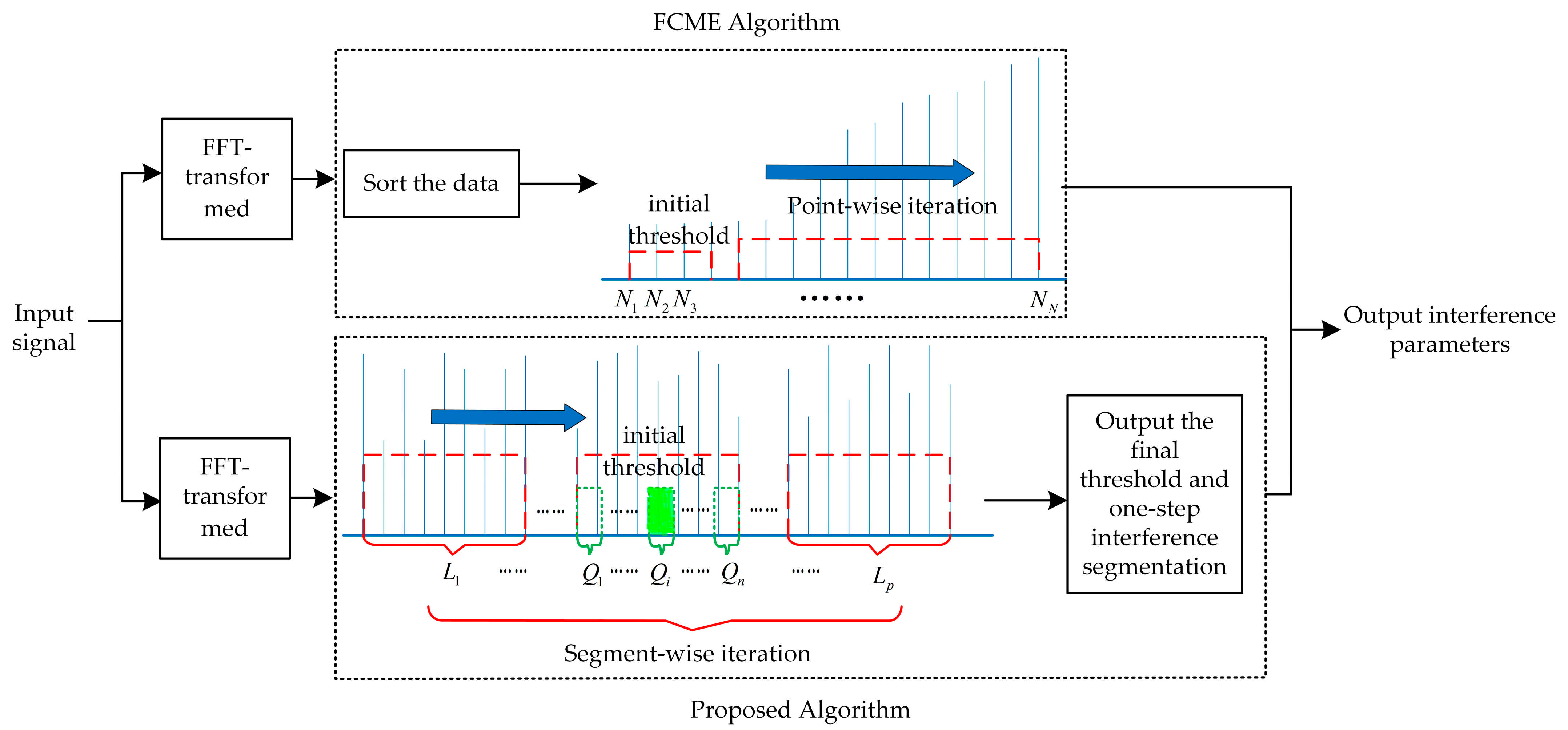
The principle of common frequency-domain interference detection algorithms is as follows: First, the input signal undergoes FFT transformation to convert the time-domain signal into the frequency domain. Then, the initial threshold is calculated, followed by iterations, and finally, the interference parameters are output. This section mainly introduces the working principles of the FCME algorithm and the proposed algorithm. Through comparative analysis, it elaborates on the similarities and differences in the processing steps of initial threshold calculation and follow-up iterations, highlighting the improvements of the proposed algorithm over the FCME algorithm. The principle comparison between the FCME algorithm and the proposed algorithm is illustrated in Figure 1.

• FCME Algorithm

First, the algorithm sorts the FFT-transformed data of length $N$ in ascending order, selecting the first 10% of frequencies as the noise set, while the remaining frequencies constitute the interference set. The initial threshold is then calculated based on the amplitudes of the frequencies in the noise set. Next, the amplitudes of the frequencies in the interference set are compared one by one with the initial threshold. Any frequencies with amplitudes smaller than the threshold are moved to the noise set, while those with larger amplitudes remain in the interference set. The threshold is then recalculated using the updated noise set, and the amplitudes of the frequencies in the updated interference set are compared with this updated threshold. The process iterates until no frequencies in the interference set have amplitudes smaller than the threshold, or the maximum number of iterations is reached, at which point the algorithm stops.

However, this algorithm requires sorting during the initial threshold calculation process. When the number of samples is large, this leads to high computational complexity and a large amount of computation. The limited memory and computational capability of satellite payloads make it difficult to support the efficient operation of this algorithm.

2.

Proposed Algorithm

This paper improves upon the limitations of the FCME algorithm by proposing an efficient differential amplitude interference detection algorithm based on non-uniform adaptive segmentation. The proposed algorithm first divides the FFT-transformed data of length $N$ into $p$ segments and uses the differential method to identify a relatively flat noise segment. The noise segment is then further subdivided into $n$ segments, and the differential method is applied again to accurately locate the final flat noise segment. The data from this flat noise segment are used to calculate the initial threshold. Next, the algorithm utilizes non-uniform data segments $L_1,L_2,\dots \dots ,Q_1,Q_2,\dots \dots ,Q_i,\dots \dots ,Q_n,\dots \dots ,L_p$, $1<i<n$ to calculate the mean amplitude of each segment, and these values are compared one by one with the initial threshold to classify the noise and interference sets. The final threshold is obtained through continuous iterations. Finally, all frequencies are compared with the final threshold and those with amplitudes greater than the threshold are classified as interference frequencies.

The proposed algorithm fully leverages the spectral characteristics of the signal by dividing it into segments of varying lengths. A two-step differential method is employed to dynamically identify the flat noise segment for initial threshold calculation and performs interference detection through segment-wise iterations. Compared to the FCME algorithm, this approach simplifies the initial threshold calculation and iterative process, making it more suitable for satellite communication systems with limited computational resources.

3.2. Specific Steps of the Proposed Algorithm

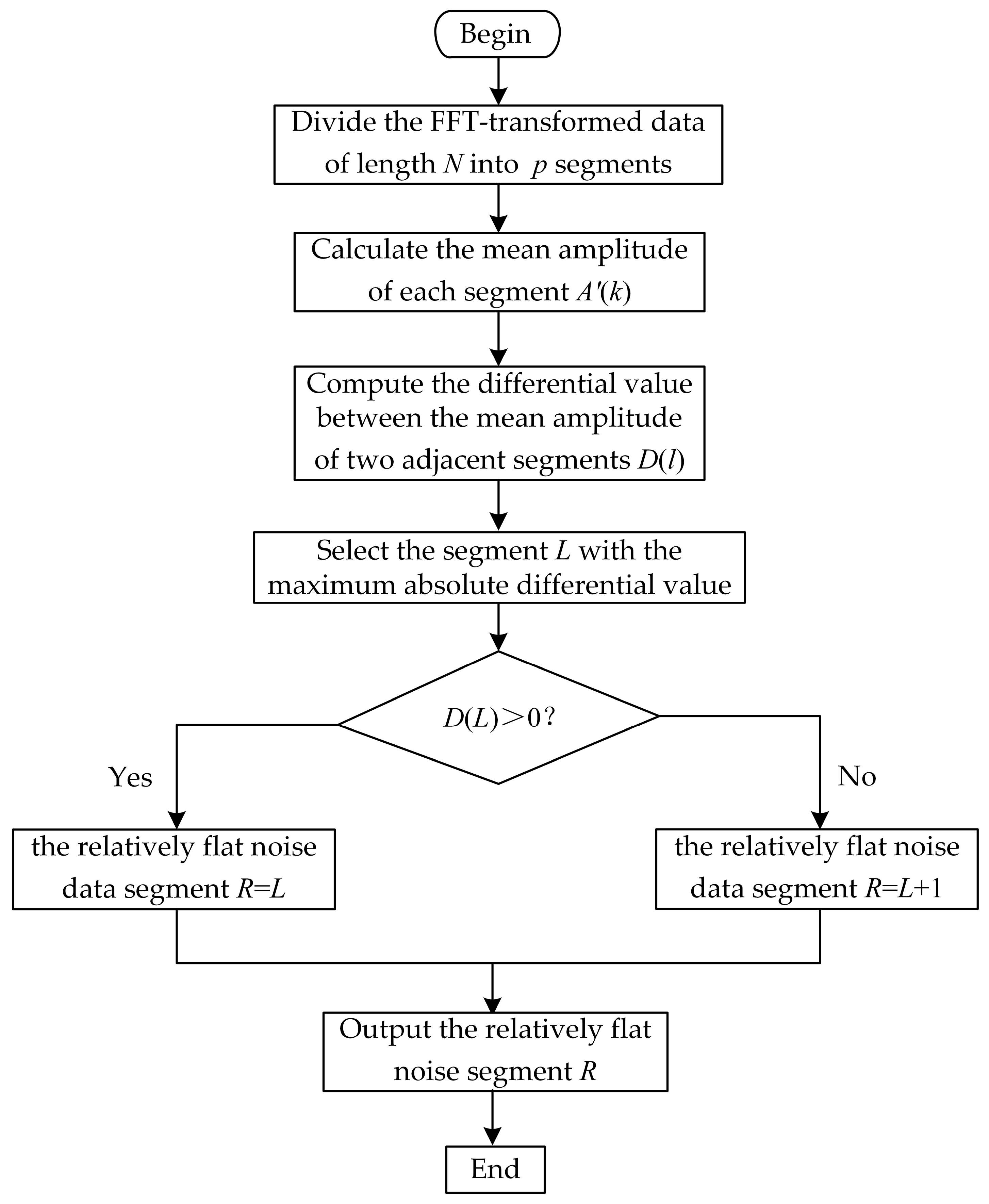
3.2.1. Steps for Calculating the Relatively Flat Noise Data Segment R

• Divide the FFT-transformed data of length N into p segments, where each segment has a length of l. Calculate the mean amplitude of each segment as follows:

  $$\begin{array}{cc}{A}^{\prime }(k)={\displaystyle \frac{1}{l}}{\displaystyle \sum _{j=1}^{l}A(l\times (k-1)+j)}& k=1,2,\dots ,p\end{array}$$

  (1)
• Compute the differential value between the mean amplitude of two adjacent segments:

  $$\begin{array}{cc}D(l)=A^{\prime }(k+1)-A^{\prime }(k)& l=1,2,\dots ,p-1\end{array}$$

  (2)
• Take the absolute value of the calculated differential value and identify the segment L with the largest absolute differential value. If the differential value is positive, the corresponding segment is considered the relatively flat noise data segment R. If the differential value is negative, the subsequent segment is considered the relatively flat noise data segment R.

The process for calculating the relatively flat noise data segment R is illustrated in Figure 2.

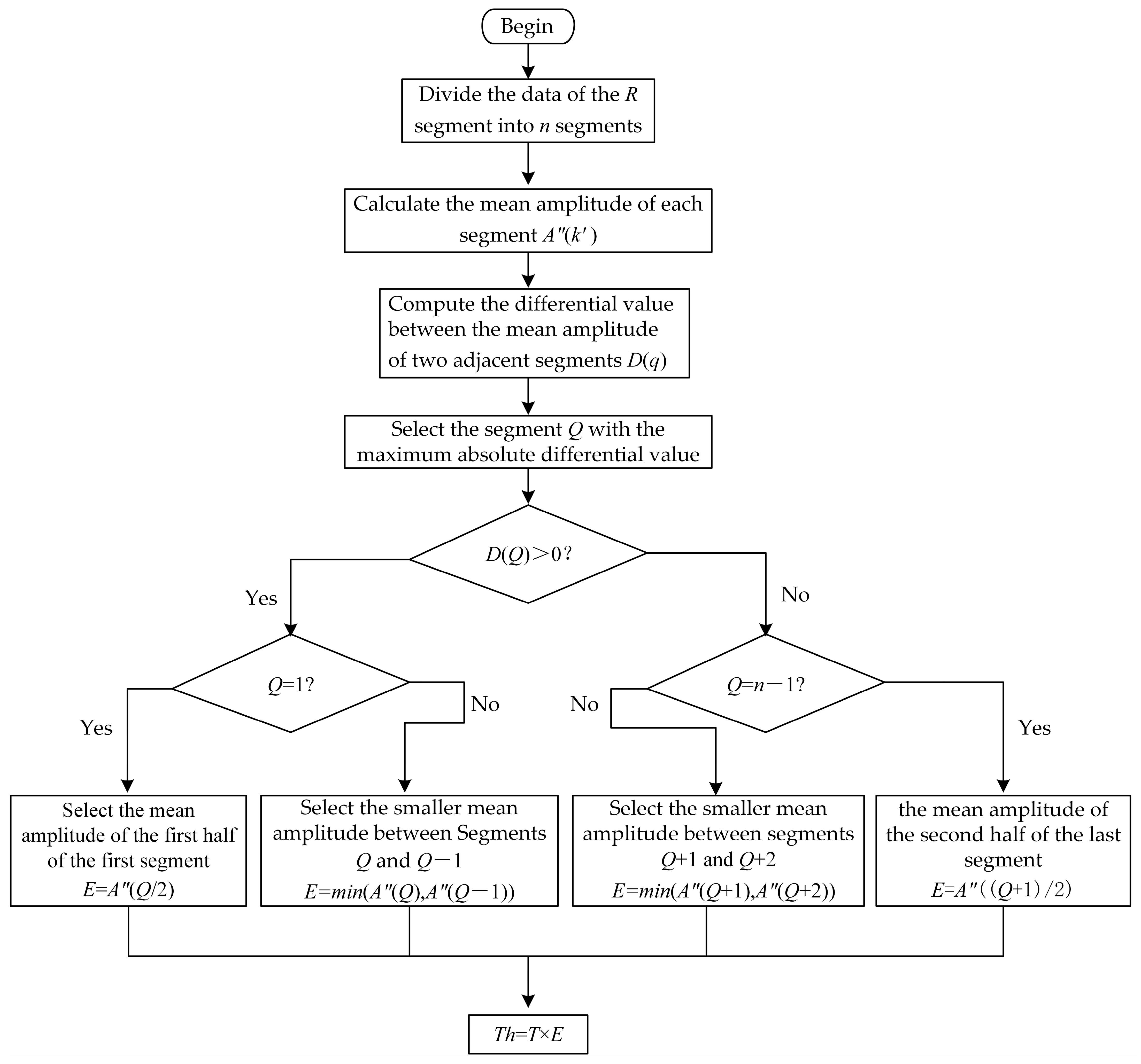
3.2.2. Steps for Initial Threshold Calculation

• Divide the data of the R segment into n segments, where each segment has a length of q. Calculate the mean amplitude of each segment as follows:

  $$\begin{array}{cc}{A}^{″}(k^{\prime })={\displaystyle \frac{1}{q}}{\displaystyle \sum _{j=1}^{q}A\left[(R-1)\times l+q\times (k^{\prime }-1)+j\right]}& k^{\prime }=1,2,\dots ,n\end{array}$$

  (3)
• Compute the differential value between the mean amplitude of two adjacent segments:

  $$\begin{array}{cc}D(q)=A^{″}(k^{\prime }+1)-A^{″}(k^{\prime })& q=1,2,\dots ,n-1\end{array}$$

  (4)
• Take the absolute value of the calculated differential value and identify the segment Q with the largest absolute differential value. If the difference value is positive, take the smaller mean amplitude between segments Q and $Q-1$ (if $Q=1$, then use the mean amplitude of the first half of the first segment). If the difference value is negative, take the smaller mean amplitude between segments $Q+1$ and $Q+2$ (if $Q=n-1$, then use the mean amplitude of the second half of the last segment).
• Multiply the calculated mean by the threshold factor T to obtain the initial threshold Th.

The process for initial threshold calculation is illustrated in Figure 3.

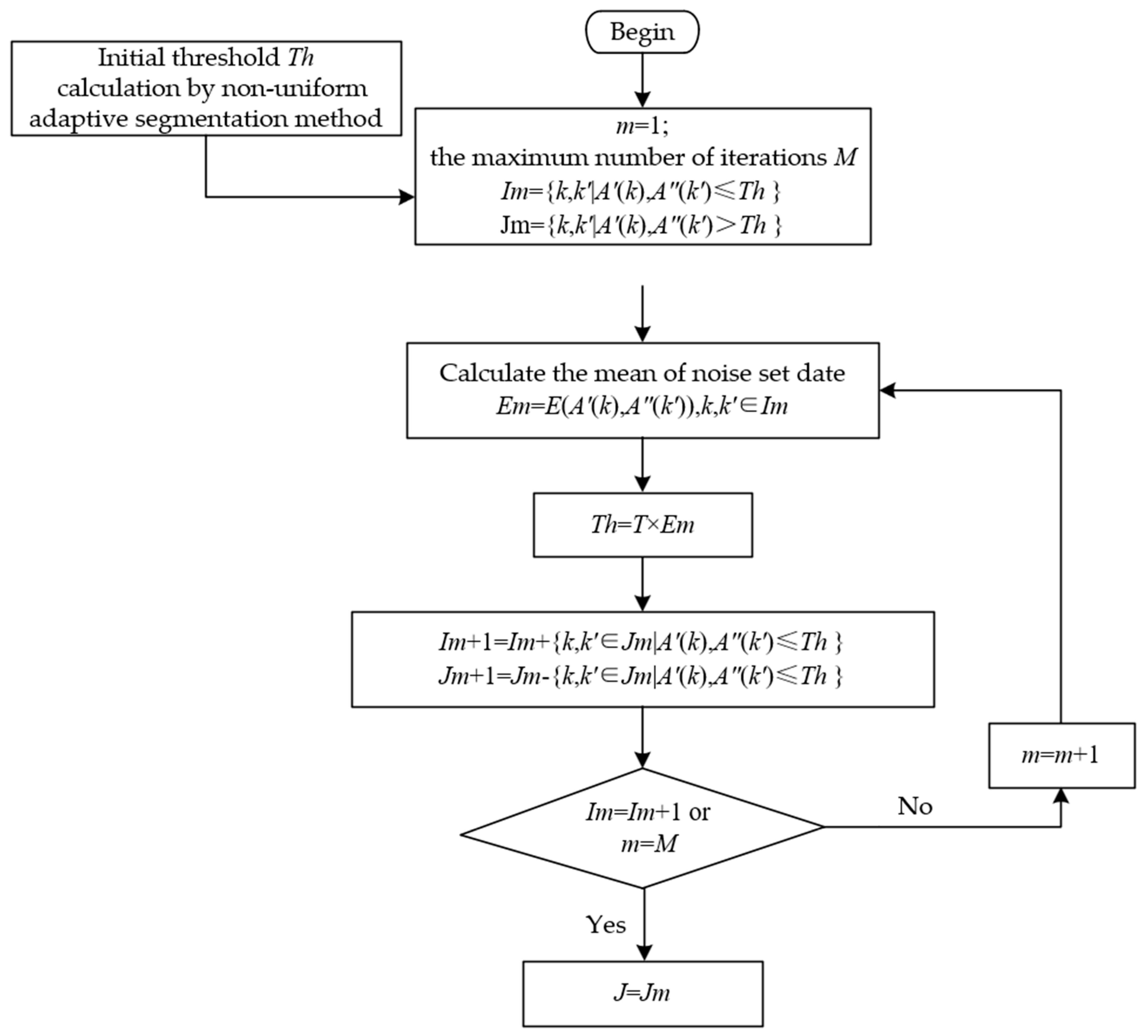
3.2.3. Steps for Iterations

• Treat the mean $A^{\prime }(k)$ of the $p-1$ segments of length $l$ and the mean $A^{″}(k^{\prime })$ of the $n$ segments of length $q$ as the interference set. Compare all data in the interference set with the initial threshold. Data smaller than the initial threshold are classified into the noise set $I_m$, while the remaining data are classified into the interference set $J_m$.
• Use the noise set $I_m$ to calculate the next threshold. Data in the interference set $J_m$ that are smaller than the new threshold are moved to the noise set, updating it to $I_{m+1}$, while the remaining data stay in the interference set, updating it to $J_{m+1}$.
• Repeat Step 2 until no new data are moved from the interference set to the noise set or the maximum number of iterations is reached, at which point the iteration stops.
• Compare the amplitude of the initial data of length $N$ with the final calculated threshold. Frequencies with amplitudes greater than this threshold are identified as interference frequencies, and the interference set $J_m$ is output.

The process for iterations is illustrated in Figure 4.

4. Simulation Results and Analysis

To validate the effectiveness of the proposed algorithm, its performance is evaluated using three indicators: detection probability, average false alarm ratio, and algorithm complexity. The proposed method is compared with the classical CME and FCME algorithms through Monte Carlo simulations to evaluate the performance of the three algorithms under single-tone interference, multi-tone interference, and partial-band interference scenarios. The simulation parameters are set as follows: FFT points $N$ = 2048; sampling frequency $f_s$ = 5 MHz; single-tone interference frequency, 1.745 MHz; multi-tone interference frequencies, 0.325 MHz, 0.7125 MHz, 1 MHz, 1.25 MHz, 1.625 MHz, and 2 MHz; the relative bandwidth (RBW) of partial-band interference is set to 10%, 50%, and 80%; and the number of Monte Carlo simulations is set to 5000. For the proposed algorithm, the two-step segmentation sizes are set as $p$ = 64 and $n$ = 2, and false alarm probability $P_f$ = 0.00001. The jammer-to-noise ratio (JNR) ranges from −35 dB to 5 dB and −10 dB to 20 dB. In this context, the relative bandwidth (RBW) is defined as the ratio of the interference signal bandwidth to the sampling signal bandwidth, while the jammer-to-noise ratio (JNR) is defined as the ratio of the interference signal power to the noise signal power.

4.1. Analysis of Detection Results for Single-Tone and Multi-Tone Interference

The detection probability is defined as the ratio of the number of times interference frequencies are correctly detected to the total number of Monte Carlo simulation runs, expressed as

$$P_d=a/5000$$

(5)

where a represents the number of times interference frequencies are correctly detected.

A higher detection probability indicates better algorithm performance, whereas a lower detection probability suggests poorer performance.

As illustrated in Figure 5, the detection performance of the CME, FCME, and the proposed algorithm is nearly identical. For single-tone interference, when JNR > −18 dB, the detection probability can approximately reach 1. For multi-tone interference, when JNR > −13 dB, the detection probability can approximately reach 1. Under the same JNR conditions, the detection probability of single-tone interference is higher than that of multi-tone interference. For the same detection probability, single-tone interference outperforms multi-tone interference by approximately 5 dB. The increase in the number of interference frequencies causes the interference signal energy to become more dispersed, thus requiring a higher JNR to achieve the same detection probability.

4.2. Analysis of Detection Results for Partial-Band Interference

In the simulation experiment, since partial-band interference is generated by white Gaussian noise passing through a bandpass filter, the resulting partial-band interference exhibits attenuation in both the side lobes and the passband. To address these issues, we define the detection probability of partial-band interference as the ratio of the number of times the correctly detected interference frequencies exceed 80% of the frequencies within the interference range to the total number of Monte Carlo simulation runs.

Figure 6 illustrates the detection probability curves for different bandwidth interferences using the three algorithms. When RBW = 10%, the detection performance of the CME, FCME, and the proposed algorithm is nearly identical. When RBW = 50%, the proposed algorithm performs about 3 dB better than the FCME algorithm, while the CME algorithm completely fails. This is because the CME algorithm assumes that all samples are free from interference when calculating the initial threshold, and as the interference bandwidth increases, the initial threshold becomes too high, making it unable to detect the interference signal. When RBW = 80%, the proposed algorithm still maintains good detection performance, whereas the CME and FCME algorithms nearly fail completely. Additionally, it can be observed that the detection performance of the algorithms decreases as the relative bandwidth increases.

4.3. Analysis of Average False Detection Rate

The average false detection rate is defined as the ratio of the average number of non-interference frequencies detected per detection run, while correctly detecting all interference frequencies, to the total number of frequencies in the signal. That is

The average false detection rate = b/2048

(6)

where b represents the average number of non-interference frequencies detected per detection run.

The lower the average false detection rate, the better the algorithm’s performance, and vice versa.

4.3.1. Analysis of Average False Detection Rate for Single-Tone and Multi-Tone Interference

In the simulation experiments, detection is performed on background noise signals with interference signals under both single-tone and multi-tone interference scenarios. For each trial, the number of frequencies exceeding the threshold is recorded, from which the number of actual interference frequencies is subtracted. The average of the remaining samples across all trials is taken as the number of non-interference frequencies.

As illustrated in Figure 7 and Figure 8, the average false detection rates of all three algorithms under both single-tone and multi-tone interferences initially increase with JNR and then gradually level off. This trend occurs because, at low JNR levels, the interference signal is not prominent enough and most of the frequencies are classified as background noise, resulting in reduced algorithm sensitivity and, consequently, lower false detection rates. As the JNR increases, the algorithms begin to detect the interference more effectively; however, they also become more prone to misclassifying non-interference frequencies as interference frequencies, causing the false detection rates to rise. When the JNR becomes sufficiently high, the interference features become more distinguishable, enabling the algorithms to accurately identify interference and reduce misclassification, leading the false detection rates to stabilize. Under single-tone interference, the average false detection rates of the three algorithms are nearly identical. Under multi-tone interference, the average false detection rates of the three algorithms, in increasing order, are as follows: CME < the proposed algorithm < FCME. Overall, the average false detection rates of all three algorithms are quite similar, and nearly zero, meaning they can be considered negligible.

4.3.2. Analysis of the Average False Detection Rate for Partial-Band Interference

In the case of noise signals under partial-band interference, the number of frequencies exceeding the threshold outside the known interference band is recorded for each trial. The average of these values across all trials is then taken as the number of non-interference frequencies.

As illustrated in Figure 9, the average false detection rates of the three algorithms also increase with the JNR at first, and then gradually level off, with the values being nearly identical across all the three methods (with similar trends as illustrated in Section 4.3.1).

4.4. Analysis of Algorithm Complexity

We will split the algorithm into two parts for analysis: initial threshold calculation and follow-up iterations. To simplify the discussion, we will focus on comparing and analyzing the parts where the three algorithms differ.

Initial Threshold: Given that the signal data length is $N$, FCME uses the Heapsort algorithm [21] for sorting, with an average time complexity of $Nlo{g}_{2}N$. The proposed algorithm divides the signal data of length $N$ into $p$ segments, then further divides a segment of length $N/p$ into $n$ segments. By incorporating the initial threshold complexity estimation method from F. Li et al.’s differential amplitude-based FCME algorithm [19], the initial threshold complexity of the proposed algorithm is $N/p+N+p+n+2$.

Follow-up Iterations: The CME algorithm compares the amplitudes of $N$ frequencies with the initial threshold one by one for classification, resulting in a complexity of $N$. The FCME algorithm compares the amplitudes of the remaining 0.9$N$ frequencies with the initial threshold one by one for classification, resulting in a complexity of 0.9$N$. Similarly, the proposed algorithm compares the mean values of the $p-1+n$ non-uniformly segmented data segments with the initial threshold, followed by a final comparison of $N$ frequency amplitudes with the final threshold. Thus, the iterative computation complexity of the proposed algorithm is $N+p+n-1$.

By adding the complexities of the initial threshold computation and the follow-up iterations, the total complexity of each algorithm is obtained. The complexity of the CME algorithm is $O(N)$, the complexity of the FCME algorithm is $O(Nlo{g}_{2}N+0.9N)$, while the complexity of the proposed algorithm is $O(N/p+2N+2p+2n+1)$.

Table 1. Comparison of algorithm complexity between FCME and oroposed algorithm.

Algorithm	Complexity	Simulation Time for Different Types of Interference (s)
		Single-Tone Interference	Multi-Tone Interference	Partial-Band Interference (10%)
CME	$O(N)$	2.307	4.658	14.566
FCME	$O(Nlo{g}_{2}N+0.9N)$	21.436	23.382	25.921
Proposed Algorithm	$O(N/p+2N+2p+2n+1)$	3.406	5.342	13.316

presents a comparison of the computational complexity and simulation time among the CME algorithm, the FCME algorithm, and the proposed algorithm. The simulation time is the cumulative time taken to perform 5000 Monte Carlo simulations for single-tone interference, multi-tone interference, and partial-band interference detection on a computer equipped with an Intel Core i5-10210U 4-core processor (Intel Corporation, Santa Clara, CA, USA) using MATLAB R2023b.

It can be seen that, compared to the CME algorithm, the proposed algorithm is slightly slower in detecting single-tone and multi-tone interference, but slightly faster in detecting partial-band interference. In contrast, compared to the FCME algorithm, the proposed algorithm improves the detection speed by nearly seven times for single-tone interference, four to five times for multi-tone interference, and nearly two times for partial-band interference. Moreover, as the number of interference frequencies increases, the detection time for both algorithms also increases. This is because a greater number of interference frequencies leads to a more dispersed interference signal energy, making it more challenging to determine the optimal segmentation threshold between interference and noise. Consequently, more iterations are required, resulting in longer detection times.

From the analysis of the above three indicators, compared with the FCME algorithm, the proposed algorithm significantly reduces computational complexity while maintaining comparable detection probability and average false detection rate. This leads to a substantial improvement in detection efficiency. In contrast, although the proposed algorithm does not show a significant advantage in computational speed over the CME algorithm under single-tone and multi-tone interference, the CME algorithm exhibits clear shortcomings in detection performance, particularly under wideband interference, where its effectiveness is notably limited. Therefore, from the perspective of adaptability to various interference types and overall performance, the proposed algorithm not only maintains robust detection capability, but also achieves higher computational efficiency. It demonstrates superior detection performance even in wideband interference scenarios, making it an interference detection algorithm that is both efficient and reliable.

5. Conclusions

To address the high complexity of existing interference detection algorithms in satellite communication systems, this paper proposes an efficient differential amplitude interference detection algorithm based on non-uniform adaptive segmentation. Simulation experiments on different types of interference signals demonstrate that, compared to the classical CME and FCME algorithms, the proposed algorithm offers superior overall performance under wideband interference conditions. In the future, we will further optimize the algorithm and explore its hardware implementation on FPGA chips to enable real-time interference detection in practical satellite communication environments, thereby enhancing system anti-interference capabilities and engineering application value.