Article

Anomalous Radio Signal Detection Based on an Adversarial Autoencoder

School of Information Engineering, Southwest University of Science and Technology, Mianyang 621000, China
*
Author to whom correspondence should be addressed.
Electronics 2025, 14(9), 1785; https://doi.org/10.3390/electronics14091785
Submission received: 26 March 2025 / Revised: 18 April 2025 / Accepted: 25 April 2025 / Published: 27 April 2025

Abstract

:
In complex and ever-changing electromagnetic environments, a large number of anomalous radio signals illegally occupy spectrum resources and interfere with legitimate communications. To address this challenge, this paper proposes an anomalous radio signal detection method based on an Adversarial Autoencoder (AAE). The method comprises an autoencoder and a Generative Adversarial Network. The autoencoder is used to extract time–frequency features of radio signals, generate latent feature vectors, and reconstruct the signals. By comparing the original signals to their reconstructions, anomalies can be rapidly and accurately detected via the reconstruction error. Meanwhile, the adversarial network regularizes the latent vectors produced by the encoder, forcing them to approximate a predefined prior distribution, thereby improving the model’s generative capability and enhancing the structural consistency of the latent representations. We used a Pluto SDR device to capture real-world radio data in the field, performed frequency-domain analysis, and constructed a high-resolution power spectrum time–frequency dataset for model training and testing. Experimental results show that the proposed method achieves a detection accuracy of 95.5% for anomalous radio signals, exhibiting excellent performance on multiple metrics across diverse scenarios.

Graphical Abstract

1. Introduction

With the rapid development of wireless communication technologies and radio devices, radio frequency spectrum resources have become an asset of critical strategic importance. As the number of spectrum-using devices increases, various anomalous radio signals continue to emerge. Generally, anomalous signals refer to those transmitted without governmental authorization or license [1], such as illegal (pirate) broadcast signals and malicious jamming. Illegal radio stations—e.g., pirate broadcasters and spoofing base stations—often disseminate objectionable content or fraudulent advertisements for profit [2]. Malicious jamming signals may be deliberately transmitted by certain individuals or organizations to disrupt legitimate communications or steal information [3], potentially causing severe consequences including communication disruptions, radar failures, and navigation signal distortion [4]. Anomalous radio signals thus seriously interfere with citizens’ day-to-day communications, endanger social stability, and even threaten national security [5]. Swift and accurate identification of anomalous radio signals is essential for ensuring uninterrupted access to broadcasting and communications, as well as maintaining national information security. Anomalous radio signal detection and identification have long been a hot topic in radio regulation research, and they continue to garner significant attention. Existing detection approaches generally fall into two major categories: parameter-based detection and deep-learning-based detection [6].
The anomalous radio detection method based on signal characteristic parameters determines the presence of anomalies by comparing the differences in characteristic parameters between the signal to be detected and the reference signal [7]. The parameters mainly include time-domain features and frequency-domain features, such as center frequency, bandwidth, signal energy, and higher-order cumulants [8,9]. However, in complex electromagnetic environments, radio signals are easily affected by random burst noise [10,11], making single-parameter anomalies insufficient for an accurate decision; more features often need to be analyzed comprehensively [12,13]. Moreover, parameter extraction can be laborious and prone to declining accuracy in highly dynamic radio environments. Purely parameter-based approaches are thus struggling to meet the growing demands for modern radio anomaly detection [14,15].
The anomalous radio identification method based on deep learning conducts anomaly identification by extracting high-level abstract feature vectors of the signals [16,17]. In practice, however, anomalous radio signals are rare [18], making it difficult to collect sufficient labeled data to support large-scale supervised training. As a result, research efforts have shifted toward unsupervised anomaly detection. In unsupervised learning, anomaly scores are generally derived from the discrepancy between the input and the model’s output [19]. Depending on how discrepancies are computed, methods can be either forecast-error-based or reconstruction-error-based. Forecast-error-based approaches predict future signal states based on historical data, then detect anomalies by comparing predicted signals against actual measurements [20,21]. Owing to the time-varying nature of radio channels, purely forecast-based methods are often unreliable. Consequently, reconstruction-based methods—where normal samples train an encoder–decoder (autoencoder) to reconstruct them accurately, and the reconstruction error is used to detect anomalies—are more popular [22]. Although this approach demonstrates good performance without requiring extensive labeled data, it can still suffer from limited representation capacity or difficulty in handling complex multimodal data distributions [23,24]. Further improving the model’s robustness under diverse anomalies remains a challenge.
To overcome these shortcomings, this paper presents an anomalous radio signal detection method based on an Adversarial Autoencoder (AAE). The autoencoder component extracts time- and frequency-domain features of signals and reconstructs them, with reconstruction errors serving as the indicator of anomalies. Meanwhile, the Generative Adversarial Network regularizes the latent vectors generated by the encoder, making them approximate a preset prior distribution, which strengthens the structural consistency of the latent representation and enhances reconstruction quality.
The contributions of the paper are mainly the following:
  • A detection scheme for anomalous radio signals based on an Adversarial Autoencoder is designed. It encompasses the extraction of features from radio signals and their high-quality reconstruction. Moreover, the detection of anomalous radio signals is accomplished by means of reconstruction error.
  • Based on software-defined radio tools, a platform for radio signal acquisition and preprocessing is established. The entire process, including signal reception, down-conversion, digitization, and FFT transformation, is completed to construct training and testing datasets.
  • By comparing the detection performance of the proposed detection method in different scenarios using real electromagnetic signal data and analyzing the detection accuracy, the advantages of the proposed detection method for anomalous radio signals are demonstrated.
The remainder of this paper is organized as follows:
Section 2 describes the structure of the proposed Adversarial Autoencoder (AAE) and its training process. Section 3 explains the radio data acquisition and dataset construction procedures. Section 4 demonstrates the system’s performance on detecting anomalous signals under different test conditions and compares it with other methods. Section 5 summarizes the main contributions and Section 6 provides a discussion on future directions.

2. Adversarial Autoencoder-Based Detection Model and Training Process

For the detection of anomalous radio signals, this paper proposes a model based on the Adversarial Autoencoder (AAE) framework. The model consists of three components: an encoder, a decoder and a discriminator. The encoder and decoder together form a standard Autoencoder (AE), which is employed to extract features from the raw input data, generate latent feature vectors, and reconstruct the input, enabling the computation of reconstruction error. Normal radio signal samples can be effectively reconstructed, resulting in low reconstruction error. In contrast, anomalous signals, which deviate from the normal data distribution, are difficult to reconstruct accurately, leading to significantly higher reconstruction errors. Therefore, anomaly detection can be achieved by applying a threshold to the reconstruction error. The encoder and discriminator constitute a Generative Adversarial Network (GAN), where adversarial training is used to regularize the latent vector distribution produced by the encoder to approximate a predefined prior distribution. This enhances the generative capability of the model and imposes structure on the latent space. The architecture of the proposed AAE model is illustrated in Figure 1.

2.1. Feature Extraction and Reconstruction Using Autoencoder

The encoder–decoder model employed in this study is a self-encoding network composed of a convolutional autoencoder and a deconvolutional decoder. The anomaly detection target in this paper is the two-dimensional time–frequency data matrix obtained by performing Short-Time Fourier Transform (STFT) on the collected spatial radio signals. Compared to time-domain and frequency-domain signals, this represents high-dimensional data. The convolutional encoder, serving as a core component of the system, is primarily responsible for transforming high-dimensional input data into low-dimensional latent feature representations. Given that radio signal time–frequency data are inherently high-dimensional and rich in temporal and spectral information, simple fully connected neural networks often struggle to capture key local features within such a vast input space, which may lead to overfitting and training instability. To address these challenges, the proposed model adopts a Convolutional Neural Network (CNN) architecture for the encoder due to its advantages in local perception and weight sharing. This design helps to significantly reduce the number of trainable parameters and enhances generalization capability during feature extraction. As illustrated in Figure 2, the encoder applies several layers of convolutional kernels to perform localized feature extraction, combined with pooling layers to gradually downsample the resolution. After several rounds of convolution and pooling, the input is compressed into a compact latent space, yielding a final low-dimensional latent vector representation.
To enhance detection accuracy and robustness, several optimization strategies were integrated into the model design. Specifically, L2 regularization was applied to the neural network layers to penalize large weight values and mitigate overfitting. Additionally, dropout layers were introduced to randomly deactivate a portion of neurons during training, preventing the network from becoming overly reliant on specific neuron activations and further reducing the risk of overfitting to the training data. Furthermore, batch normalization was applied after each convolutional or fully connected layer to normalize the activation distributions. This technique accelerates model convergence and improves training stability. The detailed architecture of the encoder is presented in Table 1.
In the structure of the Adversarial Autoencoder (AAE), the deconvolutional decoder is responsible for reconstructing the original high-dimensional time–frequency data from the low-dimensional latent vectors generated by the encoder. The decoder aims to produce reconstructed outputs that closely resemble the input data. To achieve this, transposed convolution (also known as deconvolution) and upsampling operations are employed to progressively restore the spatial resolution of the input. These techniques enable the decoder to gradually expand the latent representation back to the full resolution of the original signal. In neural networks, transposed convolutions offer flexibility in adjusting output dimensions while simultaneously learning effective feature mappings during the reconstruction process. The architecture of the deconvolutional decoder is illustrated in Figure 3.
Each layer of the decoder incorporates key operations such as transposed convolution, batch normalization, and nonlinear activation functions. The transposed convolution layers primarily serve to enlarge the spatial dimensions of the feature maps, typically using 3 × 3 kernels with a stride of 2 to ensure stable upsampling. Batch normalization is applied after each layer to regularize the output distribution, which helps prevent issues such as vanishing or exploding gradients and contributes to improved training stability. The final output layer employs a combination of linear activation and a Sigmoid function to constrain the reconstructed values within a valid range, ensuring consistency with the distribution of the original input data. With this architectural design, the decoder is capable of effectively restoring the spatial information of high-dimensional data while maintaining coherence in the generated outputs. The detailed configuration of the deconvolutional decoder is provided in Table 2.
In the encoder–decoder network, deep convolutional layers are capable of extracting multi-level feature representations, which significantly enhance the model’s ability to identify various types of anomalies. These layers can capture both complex local patterns and long-range dependencies, thereby providing higher resolution and representational power for high-dimensional spectral data. Through end-to-end training, the AAE model establishes a bidirectional mapping—from high-dimensional input data to latent vectors, and from latent vectors back to reconstructed high-dimensional data. This enables the autoencoder to effectively learn from large-scale unlabeled radio signal data and extract underlying key features and structural information. The model generates reconstructed time–frequency representations, which are then compared with the original input data to calculate the reconstruction error. For normal signals, the encoder–decoder module can accurately capture their inherent features, resulting in low reconstruction errors. In contrast, for anomalous signals, the encoder struggles to learn meaningful latent representations, limiting the decoder’s ability to reconstruct them accurately. This leads to significantly higher reconstruction errors. The reconstruction error reflects the amount of information lost during the reconstruction process and serves as a critical metric for determining whether a given radio signal is anomalous.

2.2. Adversarial Regularization of the Latent Space

In unsupervised anomaly detection tasks, the ability of an autoencoder to maintain discriminative and well-structured representations within its latent space is critical to effectively separating normal and anomalous signals. To achieve this, the proposed approach integrates the adversarial mechanism of Generative Adversarial Networks (GANs) into the autoencoder framework. Specifically, a discriminator is introduced to distinguish whether the latent vectors produced by the encoder originate from the predefined prior distribution. This adversarial interaction encourages the encoder to generate latent representations that conform to the desired distribution, thereby regularizing the latent space. Through adversarial training, the model learns the true distribution of the radio signal’s time–frequency characteristics more effectively, while also improving its generalization capability. The structure of the regularization model is illustrated in Figure 4.
The discriminator serves as a critical component within the AAE architecture. Its primary function is to determine whether a given latent vector originates from the true prior distribution or has been generated by the encoder through mapping real radio signal inputs. The discriminator is composed of multiple fully connected or convolutional layers, which are capable of extracting discriminative features from the distributional characteristics of latent vectors. To perform binary classification, the final layer of the discriminator adopts a Sigmoid activation function, enabling it to estimate the probability that an input sample belongs to the true prior distribution. The encoder and discriminator are engaged in an adversarial game: the encoder strives to “fool” the discriminator by producing latent vectors that are indistinguishable from those sampled from the true prior, while the discriminator continuously improves its ability to distinguish between the two. This adversarial process is guided by the minimization of adversarial loss, which gradually pushes the encoder’s latent outputs toward the target distribution—typically a standard normal distribution—thus achieving more effective regularization of the latent space. The structure of the discriminator used in the proposed AAE model is shown in Table 3. It consists of several fully connected layers with ReLU activations and L2 regularization. The output layer is a dense layer with a Sigmoid activation function that facilitates binary classification.
Through this mechanism, the model not only enhances its reconstruction performance for normal samples but also improves its ability to detect anomalies. Even under low signal-to-noise ratio (SNR) conditions, the model maintains stable detection performance. This approach significantly improves the robustness of radio signal anomaly detection, enabling the model to effectively distinguish between normal and anomalous signals in unsupervised learning scenarios.

2.3. Training Strategy and Optimization Workflow

The training process of the model consists of two main phases: the reconstruction phase and the regularization phase. The overall training workflow is summarized in Algorithm 1.
Algorithm 1. AAE-Based Anomaly Detection Training Steps.
Input: Time–frequency data X, prior distribution P ( z )
Output: Trained encoder E, decoder D, and discriminator Q
1.   Initialize encoder E, decoder D, discriminator Q.
2.   Repeat until convergence or max iterations:
   2.1 Pass X through AE model: X = D ( E ( X ) ) .
   2.2 Compute reconstruction loss: L recon = X X .
   2.3 Update E and D to minimize L recon .
   2.4 Encode X to latent vector Z = E ( X ) .
   2.5 Sample Z prior P ( z ) .
   2.6 Input Z, Z prior into discriminator Q.
   2.7 Compute adversarial loss L adv .
   2.8 Update E, Q to minimize L adv .
3.   Return: trained encoder E, decoder D, and discriminator Q.

2.3.1. Reconstruction Phase

The core objective of the reconstruction phase is to optimize the reconstruction capability of the autoencoder. The encoder is trained to extract key features from the input data, while the decoder is optimized to accurately reconstruct the original signal from the latent representation. By minimizing the reconstruction loss, the output of the decoder is encouraged to remain as consistent as possible with the original input data. The parameters of both the encoder and decoder are updated to minimize the reconstruction loss using stochastic gradient descent (SGD). This iterative optimization continues until the loss no longer decreases significantly or the maximum number of training epochs is reached. In this work, the Mean Squared Error (MSE) is used as the reconstruction loss, which is defined as:
L reco = 1 N i = 1 N x i x ^ i 2
In Equation (1), x i represents the i-th sample point or spectral value of the input signal, and x ^ i denotes the corresponding reconstructed value predicted by the decoder. The variable N indicates the total number of sampling points in the signal. The reconstruction loss L reco directly reflects the autoencoder’s ability to reconstruct the original signal. A smaller reconstruction loss indicates that the model can more accurately capture and reproduce the key characteristics of the input signal. At the beginning of training, the reconstruction loss is typically high, implying that the model has limited reconstruction capability. As training progresses, the model gradually learns to reconstruct the data more effectively, and the loss decreases and eventually stabilizes. If the reconstruction loss remains consistently high throughout training, it may suggest that the encoder or decoder has failed to learn meaningful representations.

2.3.2. Adversarial Regularization Phase

The regularization phase introduces an adversarial training mechanism to encourage the encoder to generate latent vectors that follow a predefined prior distribution. In this phase, a batch of real samples is drawn from a standard normal prior distribution and labeled as “real”. Simultaneously, pseudo samples are generated by passing real radio time–frequency data through the encoder, and the resulting latent vectors are labeled as “fake”. During the discriminator’s optimization, it receives both real and pseudo samples, calculates a binary classification loss, and updates its parameters to improve its discrimination ability. The goal of the discriminator is to correctly distinguish between the true prior samples and the latent vectors produced by the encoder. In contrast, the encoder is optimized to generate latent vectors that resemble the true prior distribution as closely as possible. While updating the encoder, the discriminator’s parameters are kept frozen. The encoder then minimizes the classification error made by the discriminator on the pseudo samples via backpropagation, attempting to “fool” the discriminator into believing the generated vectors originate from the real prior. As adversarial training proceeds, the encoder gradually adjusts its output such that the latent vectors increasingly match the standard normal distribution. This process improves the structure of the latent space and enhances the model’s ability to distinguish between normal and anomalous signals. To quantify the adversarial dynamics between the encoder and the discriminator, the adversarial loss is computed. It ensures that the encoder outputs latent vectors consistent with the standard Gaussian distribution. The adversarial loss consists of two components: the discriminator loss and the encoder loss.
The discriminator loss L D is calculated as:
L D = E z P z [ log D ( z ) ] E x P data [ log ( 1 D ( E ( x ) ) ) ]
The encoder’s adversarial loss L adv is computed as:
L adv = E x P enco [ log D ( E ( x ) ) ]
In the above equations, D ( · ) denotes the output of the discriminator, representing the probability that a given latent vector belongs to the target prior distribution. The distribution P z refers to the target prior, which in this study is selected as the standard normal distribution. The distribution E ( x ) corresponds to the latent vector distribution generated by the encoder.
The objective of the regularization phase is to minimize the adversarial loss L adv , thereby making it difficult for the discriminator to distinguish between true prior samples and the encoder-generated latent vectors. Through this adversarial mechanism, the encoder is forced to generate latent vectors that conform to the prior distribution, which enhances the structural consistency of the latent space. As a result, the decoder is able to generate higher-quality reconstructions that more accurately preserve the semantic content of the original input.

2.3.3. Analysis of Training Results

During model training, the RMSProp optimizer is employed to dynamically adjust the learning rate for each parameter based on gradient information. The global base learning rate η is set to 0.001, and the decay factor β is set to 0.9. This dynamic adjustment of the learning rate helps accommodate the varying gradients of different parameters, thereby ensuring efficient training while enhancing the stability of the model in complex tasks. The optimizer demonstrates strong performance when training deep neural networks, particularly in scenarios where there is a significant amount of noisy gradients or when the training data are non-stationary.
The choice of batch size has a significant impact on training stability and convergence speed. Larger batch sizes can reduce gradient noise, but they may lead to excessive memory consumption and cause convergence to flat local minima, thus compromising generalization ability. Conversely, smaller batch sizes may introduce high variance in gradient estimation, leading to unstable training. A moderate batch size was selected, and through multiple training experiments, the variations in training time, convergence speed, training stability, and test set performance were observed. Adjustments to the batch size were made to identify the optimal balance between convergence speed and model generalization. The final batch size was determined to be 64.
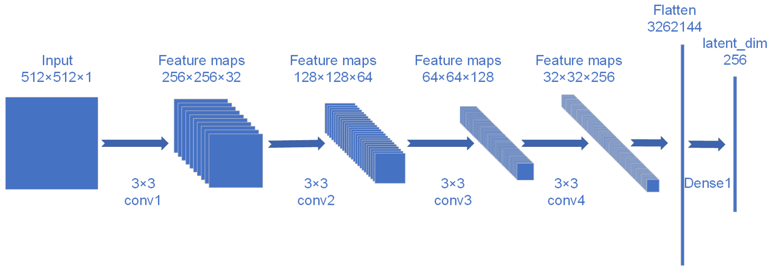
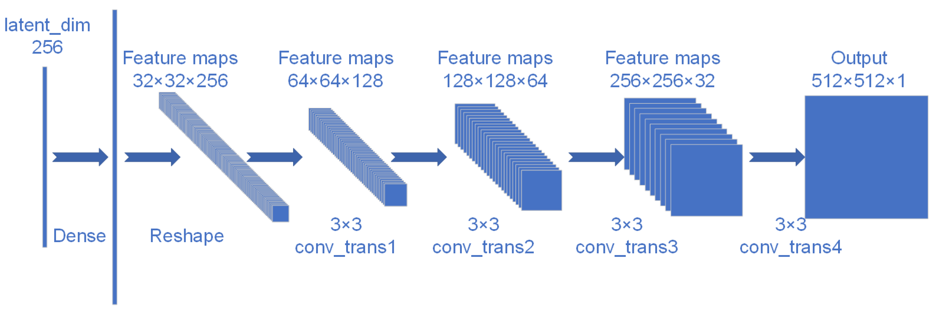
The latent space dimension in the Adversarial Autoencoder (AAE) model is a critical parameter. The input data for the model consist of single-channel images of size 512 × 512 × 1. Different latent space dimensions, such as 128, 256, 512, and 1024, were compared based on reconstruction error, discriminator performance, and generative quality. The latent space dimension of 256 was ultimately selected as the optimal configuration based on the best performance across these metrics.
During training, the model weights are saved at each epoch, allowing for reproducibility, model comparison, and recovery. An early stopping mechanism is implemented to terminate training when either the reconstruction loss or adversarial loss fails to improve significantly over 10 consecutive epochs, thereby preventing overfitting and saving computational resources.
The detailed hyperparameter settings are listed in Table 4. With a properly tuned configuration and optimization strategy, the proposed model effectively balances training complexity and generalization ability, ensuring accurate representation of normal samples while maximizing its capacity to detect anomalous signals.
The training process is illustrated in Figure 5, where all three loss values—reconstruction loss, discriminator loss, and encoder loss—are expressed in decibels (dB).
During the training process of the Adversarial Autoencoder (AAE), the reconstruction loss stabilizes after a certain number of epochs, indicating that the model has successfully learned to reconstruct the input data. The losses of the discriminator and encoder exhibit typical adversarial training behavior, where they are unstable in the early stages and then stabilize, suggesting that both components have been effectively trained. It is worth noting that the fluctuations in the loss values during the initial epochs reflect the challenges encountered during the training process. However, as the model converges, these issues are resolved. The adversarial loss guides the encoder in optimizing the distribution of the latent space, assisting the model in learning the true underlying structure of the data, while the reconstruction loss provides an evaluation of the quality of the reconstructed input data. The combination of these two losses allows the model to ensure the diversity of the generated samples while maintaining a high-quality reconstruction. The reconstruction error is a crucial parameter for subsequent anomaly detection, and the trend of the reconstruction error during training is shown in Figure 6.
At the beginning of training, the reconstruction loss is relatively high but rapidly decreases, indicating that the encoder and decoder are effectively learning the data features and gradually improving the model’s reconstruction ability. Around epoch 150, noticeable fluctuations appear in the loss curve, primarily due to the adversarial interaction between the encoder and discriminator. As the latent representations generated by the encoder begin to approach the prior distribution, the discriminator responds by adjusting its decision boundaries.
With continued training, the encoder progressively improves its ability to deceive the discriminator, and the adversarial training between the two networks reaches a stable equilibrium. Consequently, the reconstruction loss stabilizes, reflecting strong reconstruction performance and the model’s ability to accurately reproduce normal signal patterns.
Through the combination of both the reconstruction and regularization phases, the model ultimately converges to a state where it successfully balances reconstruction accuracy and latent space regularization. At this point, the learned latent representations exhibit meaningful separability, enabling the model to better distinguish between normal and anomalous samples.

3. Data Acquisition and Dataset Construction

This study focuses on the detection of anomalous radio signals within the FM broadcast frequency band (88 MHz to 108 MHz) in Mianyang City, Sichuan Province, China. This band encompasses multiple authorized FM radio transmissions, providing a solid foundation for analyzing and detecting anomalous states of licensed signals. A Pluto SDR device was used to capture ambient radio signals in the target frequency range. Fast Fourier Transform (FFT) was applied to perform frequency-domain analysis, resulting in a high-resolution power spectral time–frequency dataset. During the data acquisition process, the signal bandwidth was set to 20 MHz to fully cover the entire FM broadcast band. The key configuration parameters of the Pluto SDR are summarized in Table 5.
To shift the signal from the 88–108 MHz FM broadcast band to baseband, a local oscillator is employed to perform complex exponential downconversion. The mathematical expression is given as follows:
S down ( t ) = s ( t ) · e j 2 π f c t
In Equation (4), s ( t ) represents the received FM signal, and e j 2 π f c t is the complex exponential signal generated by the local oscillator, where f c = 98 MHz denotes the downconversion carrier frequency. After mixing, the resulting signal contains both the desired baseband components ranging from 10 MHz to + 10 MHz and undesired high-frequency image components. An IIR low-pass filter is applied to remove the high-frequency components. The passband and stopband frequencies of the filter are set to f pass = 9 MHz and f stop = 9.5 MHz , respectively. As a result, the FM radio band from 88 MHz to 108 MHz is successfully downconverted and sampled at 20 MHz. A 2048-point Fast Fourier Transform (FFT) is then performed on the filtered signal to compute the power spectral data. The frequency resolution of the FFT is calculated by the following equation:
Δ f = f s N FFT
The calculated frequency resolution is 9.77 KHz. Given a sampling frequency of 20 MHz and 2000 samples per frame, the duration of each frame is 0.1 ms. Therefore, the time resolution of the time–frequency data is 0.1 ms. The parameter settings of the collected radio signal samples are summarized in Table 6.
The time–frequency waterfall plot of the radio power spectrum is illustrated in Figure 7. This visualization intuitively presents the power distribution characteristics of various signals within the target frequency band, including the frequency locations of normal broadcast signals and the temporal variations in signal strength.
In this study, each data acquisition session lasted approximately 1.35 h, resulting in a total of 5 × 10 7 FFT samples. The ambient electromagnetic environment during acquisition was assumed to be normal, meaning that all signals were operating within their authorized specifications and no unauthorized or illegal transmissions were present. The collected radio signals under this natural electromagnetic environment were used to construct the normal-signal dataset for training the anomaly detection model. To build the dataset, 1024 consecutive time slices were randomly selected from the time–frequency data matrix, and for each slice, the first 1024 FFT data points were extracted. A channel dimension was added to match the input format required by the Convolutional Neural Network (CNN), resulting in an input shape of ( 1024 , 1024 , 1 ) . In total, 80,000 such samples were generated, forming a four-dimensional dataset with shape ( 80 , 000 , 1024 , 1024 , 1 ) for model training.

4. Experimental Evaluation

4.1. Reconstruction-Based Anomaly Detection Principle

The anomaly detection capability of the proposed model primarily relies on its ability to reconstruct the input signal. Reconstruction error reflects the discrepancy between the original input and its reconstructed version generated from compressed or low-dimensional representations. It serves as an indicator of how well the model preserves the information contained in the original signal. For normal samples, the input data closely match the learned data distribution, enabling the encoder to effectively map the signal into latent space and allowing the decoder to reconstruct it with high precision. However, if the input data deviate significantly from the training distribution, the model typically struggles to reconstruct it accurately, resulting in a noticeable increase in reconstruction error. This property enables the use of reconstruction error as a basis for anomaly detection.
In this work, the Mean Squared Error (MSE) is employed to quantify the reconstruction discrepancy. A lower MSE value indicates minimal deviation between the reconstructed and original signals, suggesting that the input is likely a normal sample. The choice of reconstruction error threshold is critical, as it defines the decision boundary between normal and anomalous signals and directly affects the overall detection performance. To balance detection sensitivity and false alarm risk, a dynamic threshold based on the 3 σ rule is adopted. The 3 σ threshold method is particularly well-suited for anomaly detection in radio signals. Given that radio signals often exhibit predictable patterns within certain ranges, the 3 σ method effectively identifies deviations from normal behavior as anomalies. This method leverages the assumption that most normal signals will fall within a specific range defined by the mean and standard deviation of the signal’s characteristics. When applied to radio signal data, this thresholding technique can efficiently highlight anomalous signals, especially when the signal characteristics follow a Gaussian or near-Gaussian distribution. According to the empirical properties of a normal distribution, approximately 99.73% of the data fall within the range of μ ± 3 σ , where μ is the mean and σ is the standard deviation. Therefore, values beyond this range have a very low probability (0.27%) of occurrence and are likely to be anomalies.

4.2. Experimental Results on Reconstruction Performance

Through the previous unsupervised training process, the model gradually learns and internalizes the distributional characteristics of normal signals. It continually improves its reconstruction capability, allowing normal signals to be accurately reconstructed from their latent representations. To evaluate the reconstruction performance, the original training dataset containing only normal signals is input into the trained model. A comparison between the original signal spectrogram and the reconstructed spectrogram is presented in Figure 8, where the horizontal axis represents frequency and the vertical axis represents time. The comparison clearly shows that the reconstructed signals preserve key characteristics of the original input, including center frequency, bandwidth, and temporal structure. This demonstrates the model’s ability to capture essential features of normal signals and verifies the effectiveness of its reconstruction capability.
In the electromagnetic environment, multiple anomalous signals were transmitted using the GNU Radio platform in conjunction with the ADALM-PLUTO hardware device. These signals were used to construct an anomalous signal dataset. By altering the modulation schemes of the transmitted signals, various illegal or anomalous modulation patterns were simulated. The signals were transmitted across multiple frequency bands to simulate multi-band anomalous signals. In addition, periodic square wave signals were transmitted to simulate pulse interference. Three different types of anomalous signal datasets were generated, each containing 1000 anomalous samples. During the experiment, 100 samples were randomly selected from the normal dataset and the three anomalous datasets. These selected samples were input into the trained Adversarial Autoencoder (AAE) model, and their reconstruction errors were computed and compared.
The reconstruction error results for normal and anomalous signals are illustrated in Figure 9 which visually demonstrates the model’s ability to distinguish between signal types based on reconstruction performance.
It can be observed that the reconstruction errors of normal signals consistently remain within a relatively low range, while the reconstruction errors of anomalous signals are significantly higher. This is because the model is trained exclusively on normal signal data, and thus only learns the underlying feature distribution of normal signals. As a result, when anomalous signals are input, the model struggles to accurately reconstruct them, leading to a substantial increase in reconstruction error.
This clear discrepancy in reconstruction error demonstrates that it can serve as an effective indicator for distinguishing between normal and anomalous signals. In practical applications, an appropriate threshold can be defined. If the reconstruction error of an input signal exceeds this threshold, the signal is classified as anomalous.

4.3. Comparative Analysis of Detection Accuracy

To evaluate the detection accuracy of the proposed system for anomalous radio signals, the three anomalous signal datasets constructed in the previous section are each combined with the normal signal dataset to form three distinct test datasets: Dataset1, Dataset2, and Dataset3.
Each test dataset is then fed into the anomaly detection system to assess its performance. The evaluation metrics for each test case, including accuracy, precision, recall, and F1-score, are presented in Table 7.
In all experiments, the precision consistently exceeds 90%, indicating that most of the samples identified as anomalous are indeed true anomalies. This demonstrates the model’s strong capability in reducing false positives. The recall also remains above 90% across all datasets, showing the model’s effectiveness in detecting actual anomalous signals. Notably, in Dataset2, the recall reaches 95.1%, further validating the model’s high sensitivity in anomaly detection. The F1-score, which serves as the harmonic mean of precision and recall, provides a balanced assessment of the model’s performance. Across the three test datasets, the F1-score ranges from 91.2% to 94.1%, indicating that the model maintains a good trade-off between precision and recall.
To further validate the detection accuracy of the proposed method, this study evaluates the performance of the Convolutional Neural Network-Adversarial Autoencoder (CNN-AAE) model, the traditional Adversarial Autoencoder (AAE) model, and the standard Autoencoder (AE) model on three test datasets containing anomalous signals. In addition, to provide a comprehensive comparison of the different methods’ performance, the Isolation Forest, K-Means Clustering, and One-Class Support Vector Machine (One-Class SVM) are also included in the comparative experiments. The comparison results are presented in Table 8.
The experimental results comparing the detection accuracy of different models across three test datasets demonstrate that the CNN-AAE model consistently outperforms other methods, exhibiting exceptional performance in handling complex anomaly detection tasks. The AAE model also demonstrates strong performance, although its accuracy shows a slight decline on Dataset3, it remains robust overall. In contrast, the AE model achieves lower accuracy, particularly on more complex datasets, indicating its limited capacity for anomaly detection. This performance gap arises because both the AAE and AE models primarily focus on frequency-domain anomalies and lack the ability to effectively capture anomalies involving temporal structures. When input signals exhibit complex time-domain variations, these traditional models struggle to reliably detect such changes. In contrast, the network structures and processes for calculating reconstruction error and anomaly detection during testing are identical for all three models, resulting in the same processing time. However, the CNN-AAE model, with its convolutional architecture, is able to learn both spectral and temporal features, allowing it to detect a wider range of subtle signal anomalies with higher accuracy and robustness. Both Isolation Forest and One-Class SVM perform well but do not surpass the deep learning models, especially in high-dimensional data. On the other hand, K-Means Clustering shows relatively lower accuracy for anomaly detection, suggesting that it is more suitable for clustering tasks rather than anomaly detection. Overall, deep learning models, particularly CNN-AAE, offer a distinct advantage in detecting anomalies in signal data.
To evaluate the model’s sensitivity to anomalies of varying signal strength, the transmission power of the FM anomaly signal generated by the vector signal source is adjusted. Anomalous datasets with different signal strengths are then collected and tested. The detection results are illustrated in Figure 10.
When the power of anomalous signals is relatively low, models generally encounter difficulties in detecting anomalies with high accuracy. This is primarily due to the associated decrease in signal-to-noise ratio (SNR), which results in less prominent feature information, thereby complicating the identification of anomalies. The detection accuracy of all models tends to decrease because, under low-power signal conditions, the models may struggle to distinguish subtle differences between normal and anomalous signals. This is particularly true for simpler spectral-based feature extraction methods, where the anomalous features of low-power signals are often overshadowed by the noise present in the normal signals.
This advantage arises from the fact that the AAE and AE models primarily focus on spectral features, which limits their ability to detect complex anomalies involving temporal components. When the input signal contains rich time-domain information, these models struggle to recognize anomalous patterns. In contrast, the CNN-AAE model captures both time and frequency features, allowing it to maintain high accuracy even under challenging low-power conditions. This demonstrates its superior robustness and adaptability to varying signal environments.

5. Conclusions

This study presents a Convolutional Neural Network-Adversarial Autoencoder (CNN-AAE) framework for the detection of anomalous radio signals based on time–frequency representations. The proposed model leverages Convolutional Neural Networks to extract spatial features from time–frequency spectrograms and employs adversarial regularization to enforce a structured latent representation. Through unsupervised training, the model learns to accurately reconstruct normal signal patterns, enabling the detection of anomalies by evaluating reconstruction errors.
Experimental results demonstrate that the CNN-AAE model achieves high detection accuracy across multiple test datasets, consistently outperforming traditional AAE and AE baselines. In particular, the model shows strong robustness against variations in signal strength, maintaining high performance under low SNR conditions. The effectiveness of the reconstruction-based detection mechanism and the regularized latent space contribute significantly to the model’s generalization capability in unseen environments. The proposed approach offers a promising solution for real-time, unsupervised anomaly detection in wireless communication systems, with potential applications in spectrum monitoring, signal intrusion detection, and cognitive radio security.

6. Discussion

Although the CNN-AAE framework demonstrates strong detection performance, there are several aspects that warrant further exploration. First, while the model effectively detects anomalies based on reconstruction error, it may be less sensitive to subtle anomalies that do not significantly alter the signal structure. Incorporating additional temporal modeling techniques could enhance the model’s sensitivity to temporal changes. For example, introducing RNN layers (such as LSTM or GRU) in the encoder or decoder could effectively capture the time dependencies and dynamic variations in the input signal, thereby enabling the model to learn temporal information. Alternatively, integrating self-attention mechanisms (such as Transformer or Self-Attention) into the encoder or decoder could allow the model to focus on important relationships between different time steps in the input sequence, dynamically adjusting the attention at each moment.
Deploying the CNN-AAE model in a real wireless monitoring system also presents several practical implementation challenges. These challenges include model training time, hardware requirements, and integration with existing wireless infrastructure. In wireless monitoring systems, the data traffic and signal characteristics are highly dynamic and variable, which necessitates frequent model training and updates, often leading to longer training cycles. The CNN-AAE model, with its complex computations, particularly in the convolutional layers and adversarial training processes, places high demands on computational resources. Integrating the model into existing wireless infrastructure requires addressing issues such as data flow management, model interface design, and ensuring compatibility with traditional wireless protocols.
When conducting radio signal anomaly detection tasks, assuming data collection under “normal” electromagnetic conditions may lead to reduced model generalization, as real-world environments are often more complex. In reality, the noise in the electromagnetic environment is dynamic, with its intensity and characteristics changing over time. Additionally, interference sources may be unpredictable or not considered during data collection. Unmodeled interference can result in decreased model performance in real-world applications. To enhance model robustness, future research should focus on data collection in various real-world environments to simulate different noise scenarios. Incorporating complex noise models (e.g., Gaussian noise, colored noise, flicker noise, etc.) can better simulate the dynamic noise characteristics found in real-world environments, ultimately improving the generalization capability of the detection model.
In summary, although the CNN-AAE model shows promising prospects for anomaly detection in wireless monitoring systems, deploying the model into real-world wireless monitoring systems presents several practical implementation challenges. Additionally, more diverse data collection scenarios and the integration of complex noise models are needed to enhance the model’s robustness and improve its generalization capability.

Author Contributions

Conceptualization, H.W. and Y.L.; methodology, Y.L.; software, Y.L.; validation, Y.L., H.W., F.L. and Y.F.; formal analysis, Y.L.; investigation, H.W. and F.L.; resources, H.W.; data curation, H.W. and Y.F.; writing—original draft preparation, Y.L.; writing—review and editing, H.W. and F.L.; visualization, Y.L.; supervision, Y.F.; project administration, H.W.; funding acquisition, H.W. All authors have read and agreed to the published version of the manuscript.

Funding

This work was supported in part by National Science Foundation grant 62261051 and Southwest University of Science and Technology PhD Fund grant 21ZX7128.

Data Availability Statement

The data presented in this study are available on request from the corresponding author. The data are not publicly available due to institutional restrictions.

Acknowledgments

The authors would like to express their sincere gratitude to the Intelligent Communication and High-Speed Signal Processing Laboratory at Southwest University of Science and Technology for providing technical support, experimental resources, and a valuable research environment throughout this study.

Conflicts of Interest

The authors declare no conflicts of interest.

Abbreviations

The following abbreviations are used in this manuscript:
AAEAdversarial Autoencoder
CNNConvolutional Neural Network
GANGenerative Adversarial Network
MSEMean Squared Error
SDRSoftware-Defined Radio
FFTFast Fourier Transform
FMFrequency Modulation
SNRSignal-to-Noise Ratio
AEAutoencoder
RFRadio Frequency

References

  1. Kim, J.; Kim, H.; Kim, B. Wireless Anomaly Signal Dataset (WASD): An Open Dataset for Wireless Cellular Spectrum Monitoring and Anomaly Detection. IEEE Access 2024, 12, 196240–196248. [Google Scholar] [CrossRef]
  2. Asikainen, E. Anomaly Detection in Radio Access Network Performance Data. Master’s Thesis, Aalto University, Espoo, Finland, 2024. [Google Scholar]
  3. Guo, J.; Xu, Y.; Zhang, M.; Huang, W.; Guo, H. Behavior Recognition and Anomaly Detection Utilizing Memory Electromagnetic Emanation. In Proceedings of the MILCOM 2024—IEEE Military Communications Conference (MILCOM), Washington, DC, USA, 28 October–1 November 2024; pp. 530–535. [Google Scholar]
  4. Bhateja, M.; Ogbe, D.; Towfic, Z. Anomaly Detection for Spacecraft Radios Based on Open-Loop Recording Data. In Proceedings of the 2024 IEEE Aerospace Conference, Big Sky, MT, USA, 2–9 March 2024; pp. 1–9. [Google Scholar]
  5. Wei, T.; Li, Y.; Niu, Y. Adversarial Sample Generation Method for Modulated Signals Based on Edge-Linear Combination. Electronics 2025, 14, 1260. [Google Scholar] [CrossRef]
  6. Xu, Y.; Zheng, K.; Liu, X.; Li, Z.; Liu, J. Cognitive Radio Networks: Technologies, Challenges and Applications. Sensors 2025, 25, 1011. [Google Scholar] [CrossRef] [PubMed]
  7. Rajeshkumar, C.; Soundar, K.R.; Muthuselvi, R.; Kumar, R.R. UTO-LAB model: USRP-based Touchless Lung Anomaly Detection Model with an Optimized Machine Learning Classifier. Biomed. Signal Process. Control 2025, 99, 106823. [Google Scholar] [CrossRef]
  8. Fan, Y.; Chen, Z.; Su, T. Anomalous Electromagnetic Radiation Detection Method for Distributed Electromagnetic Spectrum Detection System Based on RF I/Q Signal in Pre-earthquake Period. In Proceedings of the 2024 Photonics & Electromagnetics Research Symposium (PIERS), Chengdu, China, 21–25 April 2024; pp. 1–7. [Google Scholar]
  9. Perez-Portero, A.; Querol, J.; Mas-Vinolas, A.; Amezaga, A.; Jove-Casulleras, R.; Camps, A. Development of a Dynamically Re-Configurable Radio-Frequency Interference Detection System for L-Band Microwave Radiometers. Sensors 2024, 24, 4034. [Google Scholar] [CrossRef] [PubMed]
  10. Zhou, Y.; Li, J.; Gao, Y.; Wang, R.; Zhu, X.; Yu, J.; Liu, H. Electromagnetic Environment Monitoring and Analysis of the Candidate Site for the Large Array Radio Telescope. Chin. J. Radio Sci. 2024, 39, 698–705. [Google Scholar]
  11. Kim, T.-Y.; Park, E. Detecting Wireless Signal Noise in Mobile Radio Communications Using Spatiotemporal AnoGAN-Based Approaches. IEEE Can. J. Electr. Comput. Eng. 2023, 46, 310–321. [Google Scholar] [CrossRef]
  12. Anwar, U.; Khan, S.; Arslan, T.; Russ, T.C.; Lomax, P. Radio Frequency-Enabled Cerebral Blood Flow Monitoring and Classification Using Data Augmentation and Machine Learning Techniques. IEEE Sens. J. 2024, 24, 31040–31053. [Google Scholar] [CrossRef]
  13. Xu, D.; Fang, R.; Xuan, Q.; Shen, W.; Zheng, S.; Yang, X. AT-GAN: A Backdoor Attack Against Radio Signals Modulation Based on Adaptive Trigger. IEEE Trans. Circuits Syst. II Express Briefs 2024, 71, 3251–3255. [Google Scholar] [CrossRef]
  14. Yuan, A.; Zou, C.; Wang, Y.; Hu, J. Multivariate Time Series Anomaly Detection Based on Time-Frequency Dynamic Analysis. In Proceedings of the 2024 13th International Conference on Communications, Circuits and Systems (ICCCAS), Xiamen, China, 10–12 May 2024; pp. 375–379. [Google Scholar]
  15. Ye, M.; Jiang, Z.; Xue, X.; Li, X.; Wen, P.; Wang, Y. A Novel Spatiotemporal Correlation Anomaly Detection Method Based on Time-Frequency-Domain Feature Fusion and a Dynamic Graph Neural Network in Wireless Sensor Networks. IEEE Sens. J. 2025. [Google Scholar] [CrossRef]
  16. Zhang, R.; Ji, H.; Li, W.; Shang, Z.; Zhang, T. Spectrum Anomaly Detection Method Fusing Time-Frequency Attention. In Proceedings of the 2024 5th International Symposium on Computer Engineering and Intelligent Communications (ISCEIC), Wuhan, China, 23–25 August 2024; pp. 426–431. [Google Scholar]
  17. Shiri, F.M.; Perumal, T.; Mustapha, N. A Comprehensive Overview and Comparative Analysis on Deep Learning Models: CNN, RNN, LSTM, GRU. arXiv 2023, arXiv:2305.17473. [Google Scholar]
  18. Park, D.; Lee, W.; Kim, B.; Lee, J.Y. Unsupervised Learning-Based Threat Detection System Using Radio Frequency Signal Characteristic Data. J. Internet Comput. Serv. 2024, 25, 147–155. [Google Scholar]
  19. Senol, N.S.; Rasheed, A.; Baza, M.; Alsabaan, M. Identifying Tampered Radio-Frequency Transmissions in LoRa Networks Using Machine Learning. Sensors 2024, 24, 6611. [Google Scholar] [CrossRef] [PubMed]
  20. Al-Selwi, S.M.; Hassan, M.F.; Abdulkadir, S.J.; Muneer, A.; Sumiea, E.H.; Alqushaibi, A.; Ragab, M.G. RNN-LSTM: From Applications to Modeling Techniques and Beyond—Systematic Review. J. King Saud Univ. Comput. Inf. Sci. 2024, 36, 102068. [Google Scholar] [CrossRef]
  21. Wen, X.; Li, W. Time Series Prediction Based on LSTM-Attention-LSTM Model. IEEE Access 2023, 11, 48322–48331. [Google Scholar] [CrossRef]
  22. RNO-G Collaboration. Anomaly Detection in Early Data from the Radio Neutrino Observatory Greenland. In Proceedings of the 38th International Cosmic Ray Conference (ICRC2023)—Neutrino Astronomy & Physics (NU) (Proceedings of Science), Nagoya, Japan, 26 July–3 August 2024; Volume 444. [Google Scholar]
  23. Chen, X.; Deng, L.; Zhao, Y.; Zheng, K. Adversarial Autoencoder for Unsupervised Time Series Anomaly Detection and Interpretation. In Proceedings of the Sixteenth ACM International Conference on Web Search and Data Mining, Singapore, 27 February–3 March 2023; pp. 267–275. [Google Scholar]
  24. Fan, Y.; Zhang, L.; Li, K. AE-BiLSTM: Multivariate Time-Series EMI Anomaly Detection in 5G-R High-Speed Rail Wireless Communications. In Proceedings of the 2024 IEEE International Conference on Communications Workshops (ICC Workshops), Denver, CO, USA, 9–13 June 2024; pp. 439–444. [Google Scholar]
Figure 1. Architecture of the proposed CNN-AAE model for anomaly detection.
Electronics 14 01785 g001
Figure 2. CNN-based encoder structure for feature extraction.
Electronics 14 01785 g002
Figure 3. CNN-based decoder structure for data reconstruction.
Electronics 14 01785 g003
Figure 4. Adversarial regularization structure using latent vector discrimination.
Electronics 14 01785 g004
Figure 5. Training loss values over epochs.
Electronics 14 01785 g005
Figure 6. Reconstruction loss over training epochs (in decibels, dB).
Electronics 14 01785 g006
Figure 7. Waterfall plot of the time–frequency signal (in decibels, dB).
Electronics 14 01785 g007
Figure 8. Original and reconstructed time–frequency spectrograms.
Electronics 14 01785 g008
Figure 9. Reconstruction loss comparison across normal and three anomalous signal datasets (Unit: dB).
Electronics 14 01785 g009
Figure 10. Accuracy comparison under different anomalous signal strengths.
Electronics 14 01785 g010
Table 1. Encoder architecture used in the proposed AAE model.
Layer NameTypeOutput ShapeActivationRegularizationDropout
Input LayerInput(512, 512, 1)LeakyReLU
Conv1Conv2D (3 × 3, s = 2)(256, 256, 32)LeakyReLUL2(0.001)0.3
Conv2Conv2D (3 × 3, s = 2)(128, 128, 64)LeakyReLUL2(0.001)0.3
Conv3Conv2D (3 × 3, s = 2)(64, 64, 128)LeakyReLUL2(0.001)0.3
Conv4Conv2D (3 × 3, s = 2)(32, 32, 256)LeakyReLUL2(0.001)0.3
FlattenFlatten(3262144)
DenseDense(256)LeakyReLUL2(0.001)0.3
“Conv2D” refers to 2D convolutional layers with kernel size 3 × 3 and stride 2. “L2(0.001)” denotes L2 regularization with a weight decay factor of 0.001.
Table 2. Decoder architecture used in the proposed AAE model.
Layer NameTypeOutput ShapeActivationRegularizationDropout
Input LayerInput(256)LeakyReLU
Dense1Dense(3262144)LeakyReLUL2(0.001)0.3
ReshapeReshape(32, 32, 256)
Deconv1Deconv (3 × 3, s = 2)(64, 64, 128)LeakyReLUL2(0.001)0.3
Deconv2Deconv (3 × 3, s = 2)(128, 128, 128)LeakyReLUL2(0.001)0.3
Deconv3Deconv (3 × 3, s = 2)(256, 256, 64)LeakyReLUL2(0.001)0.3
Deconv4Deconv (3 × 3, s = 2)(512, 512, 32)LeakyReLUL2(0.001)0.3
Output LayerDeconv (3 × 3, s = 2)(512, 512, 1)Linear
Final Output(512, 512, 1)
“Deconv” denotes transposed convolution (Conv2DTranspose). All transposed convolutions use 3 × 3 kernels and stride 2. L2(0.001) indicates L2 regularization with a penalty factor of 0.001.
Table 3. Discriminator layer structure used in the proposed AAE model.
Layer NameTypeOutput ShapeActivationRegularizationDropout
Input LayerInput(512)NoneNoneNone
Dense1Dense(512)ReLUL2 (0.001)None
Dense2Dense(128)ReLUL2 (0.001)None
Dense3Dense(64)ReLUL2 (0.001)None
Dense4Dense(32)ReLUL2 (0.001)None
Dense5Dense(16)ReLUL2 (0.001)None
OutputDense(1)SigmoidNone
Table 4. Model hyperparameter settings.
HyperparameterValue
Learning Rate OptimizerRMSProp ( η  = 0.001,  β  = 0.9)
Batch Size64
Number of Training Epochs500 (with early stopping)
Latent Space Dimension256
Table 5. Key configuration parameters of the Pluto SDR.
ParameterValue
Center Frequency98 MHz
Baseband Sampling Rate20 MHz
Samples per Frame2000
FFT Points2048
Table 6. Signal acquisition parameters used in the experiment.
ParameterValue
Signal Acquisition Band88 MHz–108 MHz
Frequency Resolution9.77 kHz
Time Resolution0.1 ms
Baseband Sampling Rate20 MHz
Acquisition Duration5000 s
Number of Samples(50,000,000; 2048)
Table 7. Precision, recall, and F1-score of the proposed CNN-AAE model on three different anomalous signal datasets.
DatasetPrecision (%)Recall (%)F1-Score (%)
Dataset194.892.693.7
Dataset293.295.194.1
Dataset395.593.891.2
Table 8. Accuracy comparison of different models on three test datasets.
DatasetCNN-AAE (%)AAE (%)AE (%)IsoForest (%)K-Means (%)SVM(%)
Dataset196.7191.1276.3776.3980.1781.71
Dataset293.1490.2666.3473.1377.3980.24
Dataset396.6288.7363.1778.3279.0982.94
Disclaimer/Publisher’s Note: The statements, opinions and data contained in all publications are solely those of the individual author(s) and contributor(s) and not of MDPI and/or the editor(s). MDPI and/or the editor(s) disclaim responsibility for any injury to people or property resulting from any ideas, methods, instructions or products referred to in the content.

