2.3.2. Adversarial Regularization Phase
The regularization phase introduces an adversarial training mechanism to encourage the encoder to generate latent vectors that follow a predefined prior distribution. In this phase, a batch of real samples is drawn from a standard normal prior distribution and labeled as “real”. Simultaneously, pseudo samples are generated by passing real radio time–frequency data through the encoder, and the resulting latent vectors are labeled as “fake”. During the discriminator’s optimization, it receives both real and pseudo samples, calculates a binary classification loss, and updates its parameters to improve its discrimination ability. The goal of the discriminator is to correctly distinguish between the true prior samples and the latent vectors produced by the encoder. In contrast, the encoder is optimized to generate latent vectors that resemble the true prior distribution as closely as possible. While updating the encoder, the discriminator’s parameters are kept frozen. The encoder then minimizes the classification error made by the discriminator on the pseudo samples via backpropagation, attempting to “fool” the discriminator into believing the generated vectors originate from the real prior. As adversarial training proceeds, the encoder gradually adjusts its output such that the latent vectors increasingly match the standard normal distribution. This process improves the structure of the latent space and enhances the model’s ability to distinguish between normal and anomalous signals. To quantify the adversarial dynamics between the encoder and the discriminator, the adversarial loss is computed. It ensures that the encoder outputs latent vectors consistent with the standard Gaussian distribution. The adversarial loss consists of two components: the discriminator loss and the encoder loss.
The discriminator loss
is calculated as:
The encoder’s adversarial loss
is computed as:
In the above equations, denotes the output of the discriminator, representing the probability that a given latent vector belongs to the target prior distribution. The distribution refers to the target prior, which in this study is selected as the standard normal distribution. The distribution corresponds to the latent vector distribution generated by the encoder.
The objective of the regularization phase is to minimize the adversarial loss , thereby making it difficult for the discriminator to distinguish between true prior samples and the encoder-generated latent vectors. Through this adversarial mechanism, the encoder is forced to generate latent vectors that conform to the prior distribution, which enhances the structural consistency of the latent space. As a result, the decoder is able to generate higher-quality reconstructions that more accurately preserve the semantic content of the original input.
2.3.3. Analysis of Training Results
During model training, the RMSProp optimizer is employed to dynamically adjust the learning rate for each parameter based on gradient information. The global base learning rate is set to 0.001, and the decay factor is set to 0.9. This dynamic adjustment of the learning rate helps accommodate the varying gradients of different parameters, thereby ensuring efficient training while enhancing the stability of the model in complex tasks. The optimizer demonstrates strong performance when training deep neural networks, particularly in scenarios where there is a significant amount of noisy gradients or when the training data are non-stationary.
The choice of batch size has a significant impact on training stability and convergence speed. Larger batch sizes can reduce gradient noise, but they may lead to excessive memory consumption and cause convergence to flat local minima, thus compromising generalization ability. Conversely, smaller batch sizes may introduce high variance in gradient estimation, leading to unstable training. A moderate batch size was selected, and through multiple training experiments, the variations in training time, convergence speed, training stability, and test set performance were observed. Adjustments to the batch size were made to identify the optimal balance between convergence speed and model generalization. The final batch size was determined to be 64.
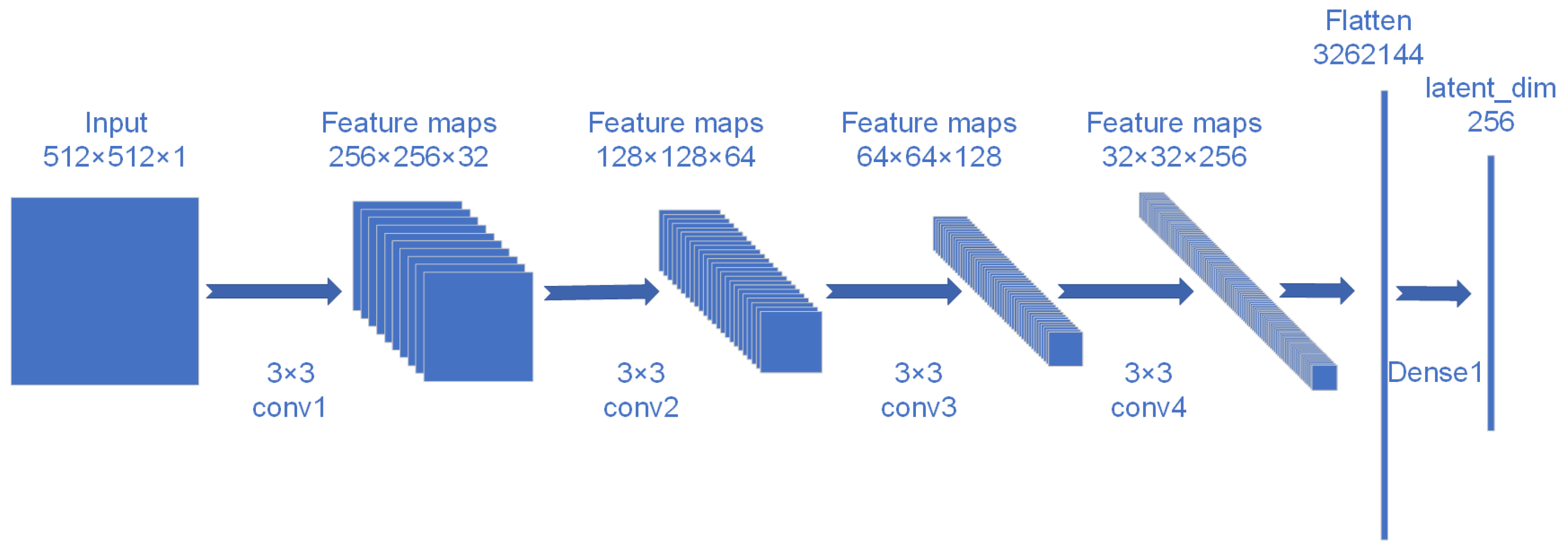
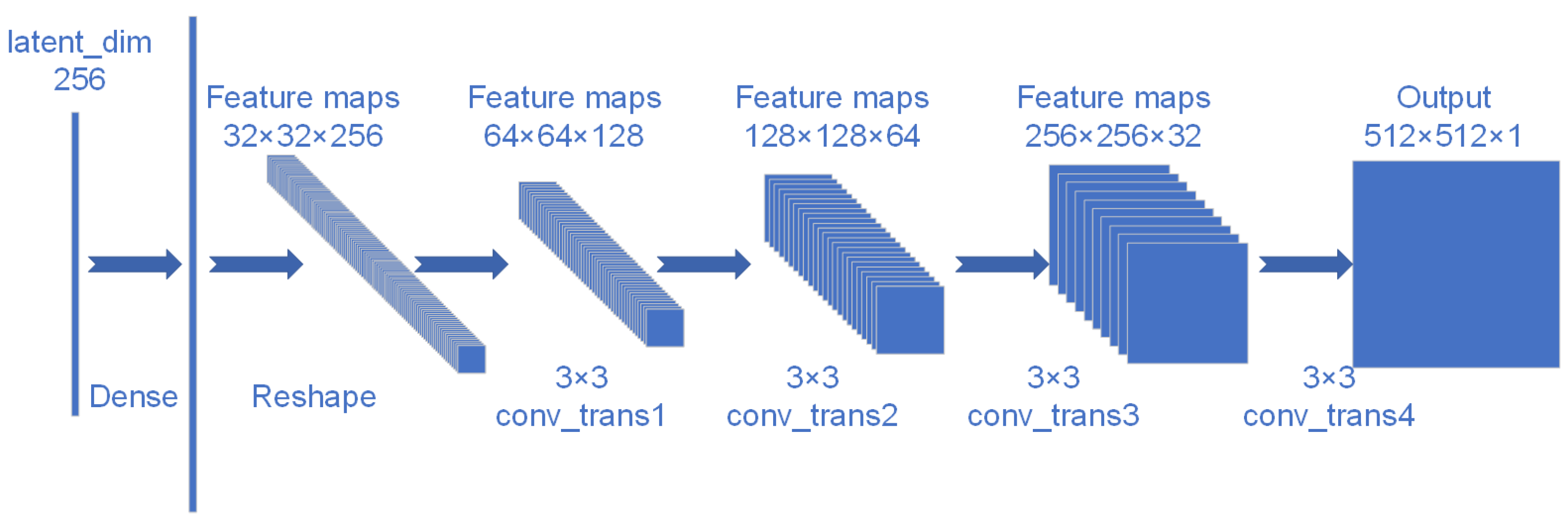
The latent space dimension in the Adversarial Autoencoder (AAE) model is a critical parameter. The input data for the model consist of single-channel images of size 512 × 512 × 1. Different latent space dimensions, such as 128, 256, 512, and 1024, were compared based on reconstruction error, discriminator performance, and generative quality. The latent space dimension of 256 was ultimately selected as the optimal configuration based on the best performance across these metrics.
During training, the model weights are saved at each epoch, allowing for reproducibility, model comparison, and recovery. An early stopping mechanism is implemented to terminate training when either the reconstruction loss or adversarial loss fails to improve significantly over 10 consecutive epochs, thereby preventing overfitting and saving computational resources.
The detailed hyperparameter settings are listed in
Table 4. With a properly tuned configuration and optimization strategy, the proposed model effectively balances training complexity and generalization ability, ensuring accurate representation of normal samples while maximizing its capacity to detect anomalous signals.
The training process is illustrated in
Figure 5, where all three loss values—reconstruction loss, discriminator loss, and encoder loss—are expressed in decibels (dB).
During the training process of the Adversarial Autoencoder (AAE), the reconstruction loss stabilizes after a certain number of epochs, indicating that the model has successfully learned to reconstruct the input data. The losses of the discriminator and encoder exhibit typical adversarial training behavior, where they are unstable in the early stages and then stabilize, suggesting that both components have been effectively trained. It is worth noting that the fluctuations in the loss values during the initial epochs reflect the challenges encountered during the training process. However, as the model converges, these issues are resolved. The adversarial loss guides the encoder in optimizing the distribution of the latent space, assisting the model in learning the true underlying structure of the data, while the reconstruction loss provides an evaluation of the quality of the reconstructed input data. The combination of these two losses allows the model to ensure the diversity of the generated samples while maintaining a high-quality reconstruction. The reconstruction error is a crucial parameter for subsequent anomaly detection, and the trend of the reconstruction error during training is shown in
Figure 6.
At the beginning of training, the reconstruction loss is relatively high but rapidly decreases, indicating that the encoder and decoder are effectively learning the data features and gradually improving the model’s reconstruction ability. Around epoch 150, noticeable fluctuations appear in the loss curve, primarily due to the adversarial interaction between the encoder and discriminator. As the latent representations generated by the encoder begin to approach the prior distribution, the discriminator responds by adjusting its decision boundaries.
With continued training, the encoder progressively improves its ability to deceive the discriminator, and the adversarial training between the two networks reaches a stable equilibrium. Consequently, the reconstruction loss stabilizes, reflecting strong reconstruction performance and the model’s ability to accurately reproduce normal signal patterns.
Through the combination of both the reconstruction and regularization phases, the model ultimately converges to a state where it successfully balances reconstruction accuracy and latent space regularization. At this point, the learned latent representations exhibit meaningful separability, enabling the model to better distinguish between normal and anomalous samples.

