An Effective Mixed-Precision Quantization Method for Joint Image Deblurring and Edge Detection

Abstract

Deploying deep neural networks (DNNs) for joint image deblurring and edge detection often faces challenges due to large model size, which restricts practical applicability. Although quantization has emerged as an effective solution to this issue, conventional quantization methods frequently struggle to optimize for the unique characteristics of the targeted model. This paper introduces a mixed-precision quantization method that dynamically adjusts quantization precision based on the edge regions of the input image. High-precision quantization is applied to edge neighborhoods to preserve critical details, while low-precision quantization is employed in other areas to reduce computational overhead. In addition, a zero-skipping computation strategy is designed for model deployment, thereby enhancing computational efficiency when processing sparse input feature maps. The experimental results demonstrate that the proposed method significantly outperforms existing quantization methods in model accuracy across different edge neighborhood settings (achieving 97.54% to 98.23%) while also attaining optimal computational efficiency under both 3 × 3 and 5 × 5 edge neighborhood configurations.

1. Introduction

Edge detection is a fundamental task in advanced image processing [1,2,3,4,5]. When dealing with motion-blurred images, effective image deblurring techniques are crucial for enhancing edge detection accuracy. With significant advances in deep learning, recent approaches using DNNs for image deblurring have achieved remarkable success, making them a key area of focus in this field [6,7,8,9,10,11]. However, in applications involving industrial defect detection, mobile robotics, and autonomous driving, there is a strong demand for real-time algorithm performance [12,13,14]. Given the substantial parameter and computational requirements of DNNs, the integration of image deblurring and edge detection places a significant burden on memory and processing resources, potentially hindering real-time performance. Therefore, efficient strategies are required to address this challenge.

Most researchers employ model compression techniques to reduce model complexity and improve computational efficiency, with representative methods including low-rank decomposition, knowledge distillation, pruning, and quantization [15]. Among these, quantization compresses networks by representing model parameters and feature maps using low-precision-quantized integer values [16,17], thereby significantly reducing model size without altering the network architecture. Nonetheless, due to the information loss induced by low-precision representations, quantization may lead to model accuracy degradation. Driven by the real-time performance requirements of motion-blurred image edge detection tasks, this research aims to develop a quantization method that reduces model complexity while maintaining model accuracy.

Early studies primarily adopted uniform low-bit quantization, compressing model precision from FP32 down to INT8 or even INT2. This approach applies the same low-bit precision across all layers or parameters, thereby significantly reducing model size and accelerating inference. Representative methods in this direction include binary quantization such as BinaryConnect [18] and ABC-Net [19], as well as ternary quantization like TWN [20] and TTQ [21]. While these approaches efficiently decrease computational complexity and memory usage, they do not account for the diverse sensitivity of different layers or feature maps. As a result, layers that are more sensitive to quantization errors may suffer noticeable performance degradation. Moreover, strict uniform quantization strategies often limit fine-grained control over bit-width distribution, constraining the achievable balance between accuracy and speed.

To achieve a more flexible trade-off between model complexity and accuracy, researchers have explored mixed-precision quantization, where certain layers are assigned higher bit-widths while others use lower bit-widths. By allocating more bits to layers that are particularly sensitive to quantization errors, these methods can substantially mitigate accuracy loss compared to uniform quantization, thereby achieving higher accuracy under real-time constraints. The key challenge in this process is determining the optimal bit-width configuration for each layer. HAQ [22] employs reinforcement learning to navigate the extensive space of layer-wise weight and activation bit-width assignments and identify an optimal setting, while DNAS [23] uses random sampling from a super-network to jointly optimize bit-widths and network architecture. Furthermore, HAWQ [24], PyHessian [25], and Q-BERT [26] analyze the Hessian matrix to identify which layers are most sensitive to quantization errors, allocating more bits to these layers to mitigate accuracy loss. However, these quantization methods are primarily applied at the inter-layer level and often lack fine-grained optimizations that are tailored to the particular model being employed.

Meanwhile, existing research indicates that input feature maps do not exert a uniform impact on overall network performance [27,28]. To advance mixed-precision quantization even further, recent studies have investigated intra-layer quantization strategies that allow multiple precision settings within the same layer. For example, AutoQ [29] leverages reinforcement learning to determine kernel-level bit-widths, while DRQ [30] dynamically adjusts the precision of DNN models based on sensitive regions in feature maps, achieving fine-grained intra-layer mixed precision. Motivated by these findings, this paper proposes an effective quantization method for joint image deblurring and edge detection, making the following key contributions:

• A fine-grained mixed-precision quantization method is introduced, enabling the dynamic adjustment of quantization precision across different regions of input feature maps;
• To ensure efficient computation when the input feature map is sparse, a zero-skipping computation strategy is proposed for model deployment;
• The quantized model is deployed on an FPGA platform, demonstrating both improved inference speed and high accuracy in comparative experiments, thus validating the effectiveness of the proposed method.

2. Methods

2.1. Quantization Method Based on Edge Neighborhood

Previous studies have shown that different regions of the input feature map contribute differently to the accuracy of a neural network [30]. A small subset of key regions plays a crucial role in maintaining network performance and is most sensitive to quantization errors. Specifically, in a joint image deblurring and edge detection task, the edge and its surrounding neighborhood often contain essential information, such as object contours and fine details, which directly impact the accuracy of detection. Additionally, edge-neighboring regions exhibit sharp intensity variations and high gradient values, which not only serve as significant features for edge determination but also play a critical role in both forward and backward propagation within the network. Therefore, we identify edge neighborhoods as the regions most sensitive to quantization errors. To determine these sensitive regions, we first perform initial edge detection on the input image. Based on the detected edge points, we expand a fixed-size neighborhood around them to obtain the complete set of sensitive regions. Finally, we apply high-precision quantization to these error-sensitive edge neighborhoods, while employing low-precision quantization for the remaining regions that exhibit higher tolerance to quantization errors. These steps form the quantization method illustrated in Figure 1.

Initially, we conduct both high-precision and low-precision quantization-aware training (QAT), which yields two quantized models: a high-precision-quantized model and a low-precision-quantized model. Without a loss of generality, our high-precision model uses 8-bit symmetric linear quantization: weights are quantized per channel (range [−127, 127]) to minimize quantization error, while activations are quantized per layer (range [0, 255]) to improve hardware efficiency; the low-precision model simply reduces the bit-width to 4 bits—mapping weights to range [−8, 7] and activations to range [0, 15]—while all other quantization settings remain identical.

To guide our deblurring process, we first apply the Canny edge detection algorithm [31] to extract an edge mask from the motion-blurred image. In this study, we used the following parameter settings: Gaussian smoothing with a 3 × 3 kernel and σ = 1.0; hysteresis thresholds of 50 (low) and 150 (high) on a 0–255 scale; and an edge neighborhood expansion size of 3. Based on this edge mask, we generate two distinct feature maps. The first feature map, referred to as the Edge Neighborhood Map, retains the pixel values of the edge mask along with those in its m × m neighborhood, while setting all other pixel values to zero. The second feature map, called the Inverse Edge Neighborhood Map, does the opposite—it sets the pixel values of the edge mask and its m × m neighborhood to zero, preserving only the pixel values in the remaining regions. Each of these feature maps is then processed independently using different quantized models: the high-precision model for the Edge Neighborhood Map and the low-precision model for the Inverse Edge Neighborhood Map. The outputs from these two branches are subsequently combined to produce the initial deblurred result. Finally, we apply the Canny edge detection algorithm once more to the combined output to obtain an enhanced edge detection result for the motion-blurred image.

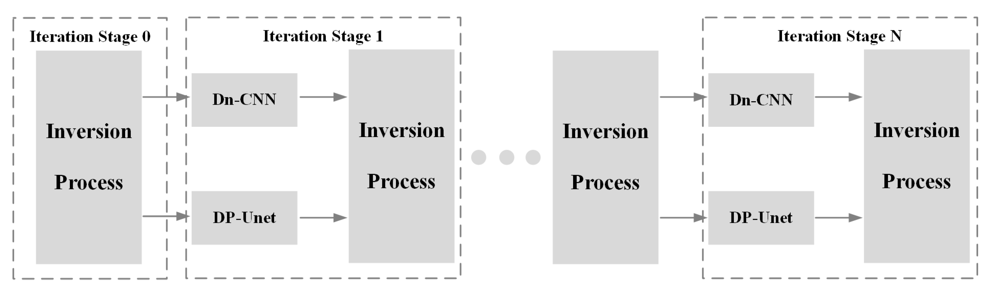
2.2. Workflow for Model Deployment

In our proposed quantization method, models with both high- and low-precision quantization are derived through the workflow depicted in Figure 2 and ultimately deployed on FPGA devices. The workflow consists of two main stages: quantization-aware training based on the Xilinx Brevitas library, and model conversion and deployment based on the FINN framework [32].

First, the Brevitas library is employed to apply quantization parameters to standard PyTorch layers (version: 1.13.1), systematically reducing the model to different bit-width representations, including 8-bit, 4-bit, and 2-bit precision. Quantization-aware training is then conducted on the prepared dataset, optimizing the performance of the quantized models to mitigate accuracy loss resulting from quantization. Upon completion of training, the quantized model is exported to Quantized Open Neural Network Exchange (QONNX) format [33], ensuring compatibility with subsequent tools in the deployment process.

The QONNX-exported model is subsequently converted into a hardware-synthesizable dataflow graph format using the ModelWrapper() function as part of the broader model transformation workflow in FINN. Next, the dataflow graph is translated into hardware description language (HDL) code through Vivado High-Level Synthesis (HLS), preparing it for FPGA synthesis. Through the adjustment of parameters such as processing element (PE) and SIMD width, parallelism and resource utilization can be optimized for the specific application requirements. The generated HDL code is then synthesized into an FPGA bitstream using Vivado 2022.2, ensuring compatibility with the target FPGA platform. Additionally, a custom driver is developed to facilitate communication between the host CPU and FPGA, and the necessary runtime files are prepared and loaded onto the target device.

Finally, the bitstream file and the custom driver are deployed on the target FPGA platform, and the model can be run on the platform using the PYNQ framework.

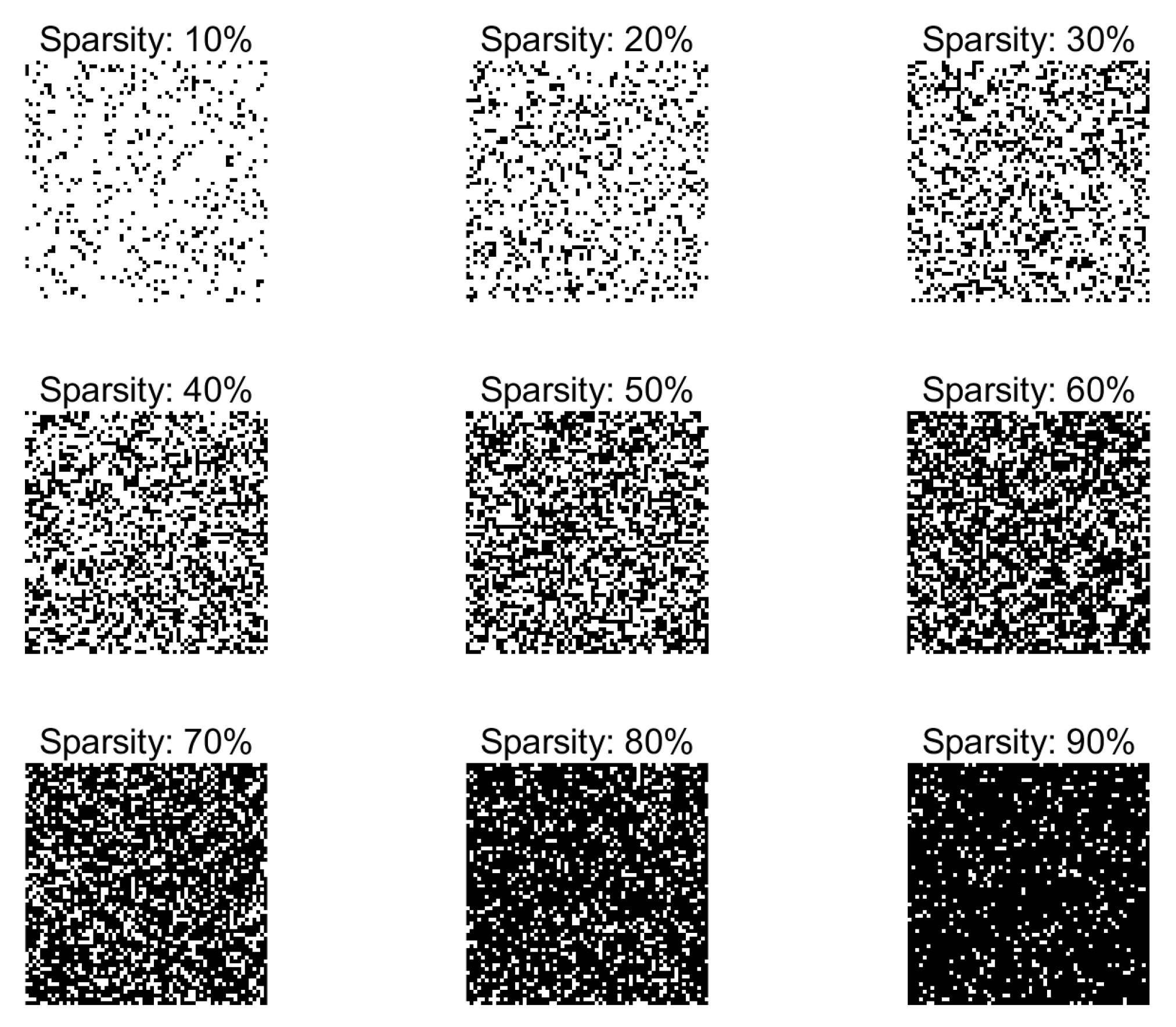
2.3. Zero-Skipping Computation

Once the model is deployed using the proposed quantization method, the bottleneck for improving computation efficiency primarily comes from the high-precision-quantized model, which incurs the largest computational load. Given that the Edge Neighborhood Map, which serves as the input for the high-precision-quantized model, is predominantly composed of zero values, we developed a zero-skipping computation method, illustrated in Figure 3, to effectively reduce inference time for sparse inputs.

The proposed zero-skipping computation method is primarily aimed at convolutional neural networks (CNNs). Since the main computational load of CNN models is in the convolutional layers, we designed the zero-skipping operation specifically for convolutional computation. In the FINN framework, the computation of convolutional layers is converted into two steps: Im2Col (Image to Column) and MatMul (Matrix Multiplication). The Im2Col operation transforms the input feature map into a Flattened Input Matrix, where each column represents a flattened region of the input that corresponds to the receptive field of a convolution kernel, as illustrated in Figure 3a.

Let the input feature map be $\mathit{X}\in {ℝ}^{C_{in}\times H_{in}\times W_{in}}$, where $C_{in}$ is the number of input channels, and $H_{in}$ and $W_{in}$ are the input height and width. The convolution kernel is $\mathit{W}\in {ℝ}^{K\times C_{in}\times K_h\times K_w}$, where K is the number of output channels (i.e., number of convolution kernels), and $K_h$ and $K_w$ are the height and width of the convolution kernel.

After the Im2Col transform, the input tensor is rearranged into the Flattened Input Matrix:

$${\mathit{X}}_{flat}\in {ℝ}^{(C_{in}{K}_h{K}_w)\times \left(H_{out}{W}_{out}\right)},$$

(1)

where $H_{out}$ and $W_{out}$ are the height and width of the output feature map, determined by the input feature-map size, kernel size, stride, and padding settings. For multi-channel inputs ($C_{in}>1$), the Im2Col operation concatenates the $K_h{K}_w$ patches from all $C_{in}$ channels into each column of ${\mathit{X}}_{flat}$. Consequently, each column vector has length $C_{in}{K}_h{K}_w$ and contains the flattened values from every input channel at a single spatial location.

Likewise, every convolution kernel is stacked into a row vector, forming the Flattened Kernel Matrix:

$${\mathit{W}}_{flat}\in {ℝ}^{K\times \left(C_{in}{K}_h{K}_w\right)}.$$

(2)

In the MatMul operation, the convolution is compactly expressed as

$${\mathit{Y}}_{flat}={\mathit{W}}_{flat}{\mathit{X}}_{flat}, {\mathit{Y}}_{flat}\in {ℝ}^{K\times \left(H_{out}{W}_{out}\right)}.$$

(3)

To implement the zero-skipping computation, after the Im2Col operation, we output an additional 1 × N zero-skipping mask along with the Flattened Input Matrix.

$$\mathit{M}\in {\left\{0, 1\right\}}^{1\times \left(H_{out}{W}_{out}\right)}, M_j=\{\begin{array}{c}0, {\Vert {\mathit{x}}_j\Vert }_0=0, \\ 1, otherwise. \end{array}$$

(4)

When a column of the matrix has all values as zero, the corresponding entry in the zero-skipping mask is also zero; otherwise, it is set to one, as shown in Figure 3b. During the MatMul operation, based on the zero-skipping mask, the multiplication and accumulation operations for the column vectors with a mask value of zero are skipped. Let the column-level sparsity be

$$\rho =1-{\displaystyle \frac{{\Vert \mathit{M}\Vert }_0}{H_{out}{W}_{out}}}.$$

(5)

The theoretical multiply–accumulate (MAC) count of this convolution layer is reduced from

$$MA{C}_{ori}=K{C}_{in}{K}_h{K}_w{H}_{out}{W}_{out}.$$

(6)

to

$$MA{C}_{ZS}=K{C}_{in}{K}_h{K}_w\left(1-\rho \right)(H_{out}{W}_{out})=\left(1-\rho \right)MA{C}_{ori},$$

(7)

For CNN models, when input images exhibit high sparsity, the feature maps generated after the initial convolutional layers tend to preserve this sparse characteristic. Consequently, zero-skipping acceleration techniques accumulate computational efficiency gains across multiple network layers, effectively reducing the computation.

Note that in FINN’s fully streaming architecture, no full output matrix ${\mathit{Y}}_{flat}$ is ever materialized on-chip between layers. Each column vector produced by one MatMul IP is streamed directly into the next layer’s Im2Col unit. Only after the final convolutional layer is the complete one-dimensional stream transferred off-chip to external DRAM. The host then takes this flat sequence—whose logical shape is $K\times \left(H_{out}{W}_{out}\right)$—and reshapes it into a feature map of dimensions $K\times H_{out}\times W_{out}$, thereby reconstructing the final output tensor.

3. Experiments

3.1. Experiments for Zero-Skipping Computation

To verify the effectiveness of the proposed zero-skipping acceleration method, we conducted experiments on two architectures: a simple CNN consisting of a single convolutional layer and the more complex Dn-CNN which was introduced in [34]. This allowed us to evaluate the acceleration benefits across both shallow and deeper networks, demonstrating the generalizability of our approach. Since accuracy testing was not a focus, the quantization-aware training step was omitted. The network parameters were randomly initialized, and subsequently, the model was quantized to 8-bit precision using the Brevitas library. The quantized model was then converted and deployed on the Xilinx Zynq UltraScale+ MPSoC ZCU102 development board using the FINN framework, which had been modified to include the zero-skipping functionality.

The input data consisted of 64 × 64 binary matrices, with sparsity (i.e., the proportion of elements that are zero) incremented from 10% to 90% in increments of 10%. The effectiveness of the zero-skipping acceleration method was verified by measuring the computation time of the model for input matrices with varying levels of sparsity. The input matrices with different sparsity levels and their corresponding computation times are illustrated in Figure 4 and Figure 5. Specifically, as the sparsity increases from 10% to 90%, the computation time gradually decreases from 1.20 × 10⁻⁴ s to 3.86 × 10⁻⁵ s for the single-layer CNN and from 1.01 × 10⁻³ s to 5.82 × 10⁻⁴ s for the Dn-CNN. These results demonstrate that the zero-skipping acceleration method can significantly reduce the computational load for highly sparse input data, thereby significantly improving model inference speed.

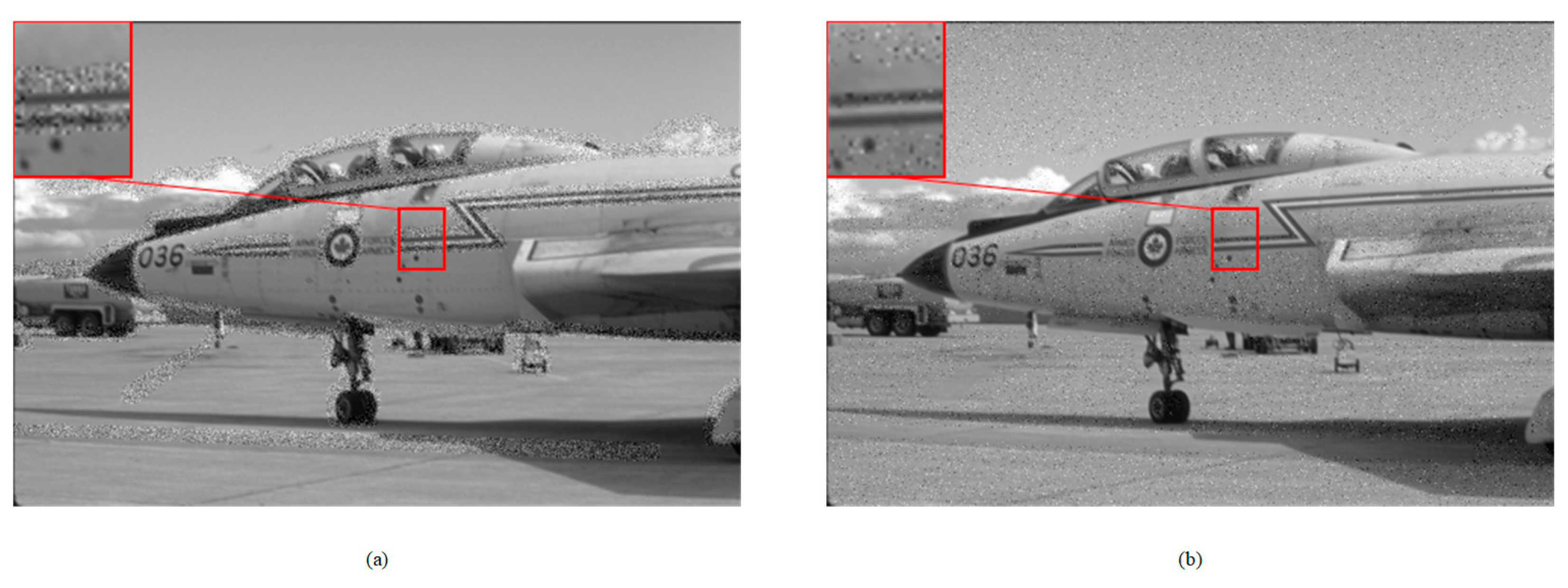
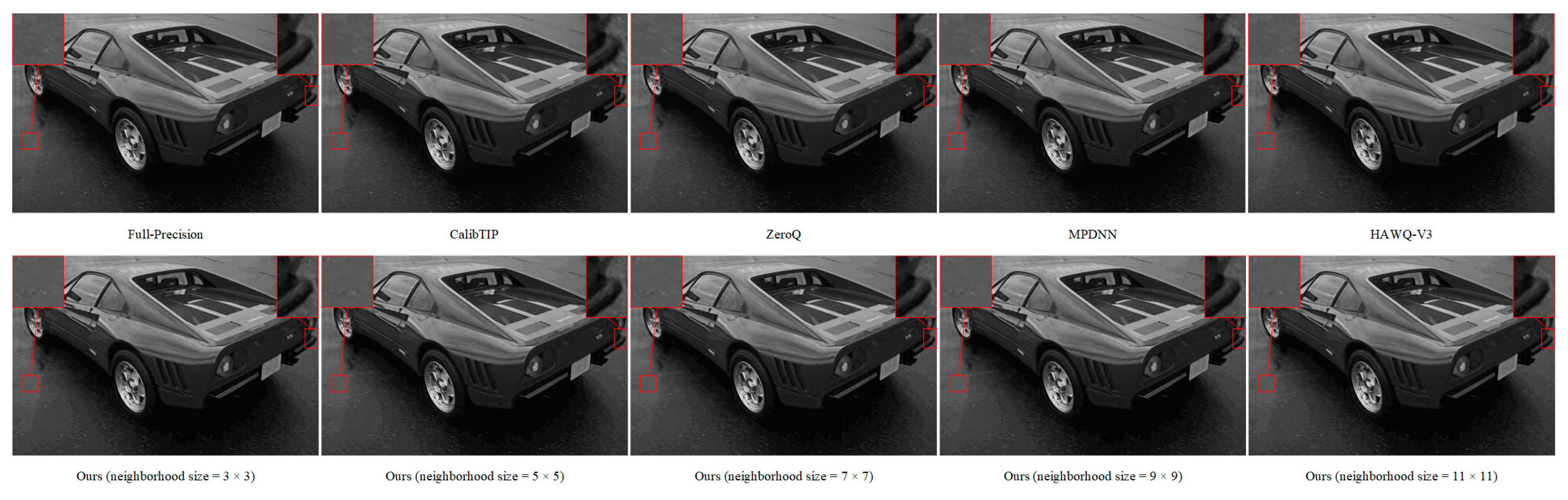
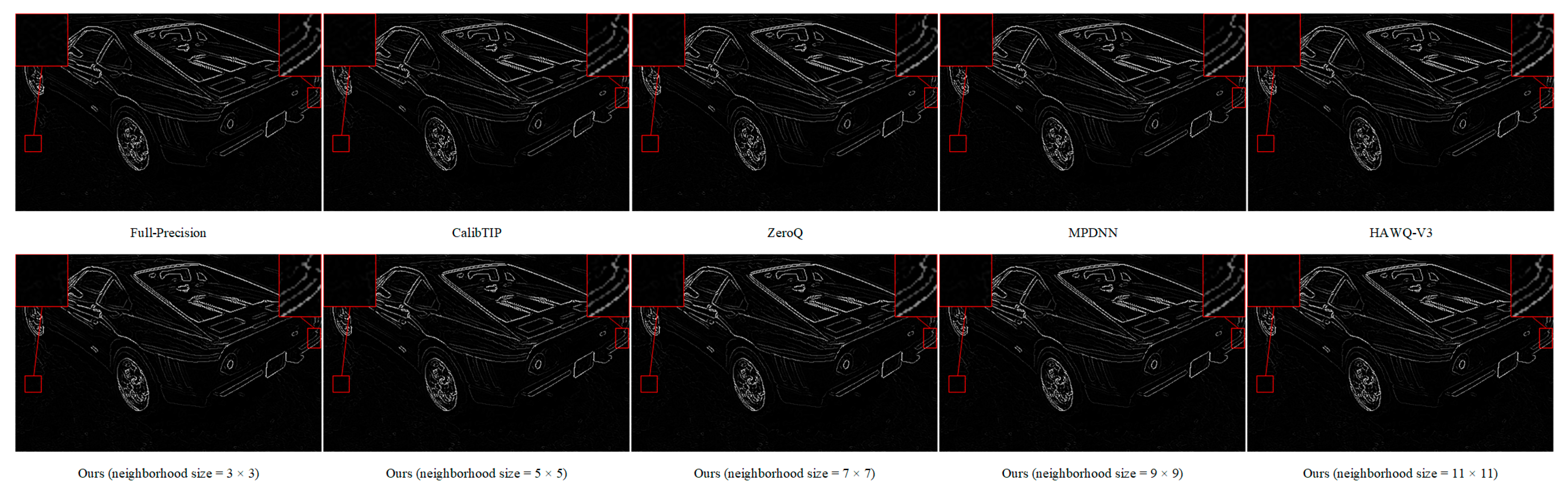
3.2. Experiments for Joint Image Deblurring and Edge Detection

In our prior work [35], we proposed a deblurring method tailored for edge detection tasks. This approach, built on an iterative optimization algorithm, effectively handles blur-kernel errors during the deblurring process, thereby ensuring the method’s robustness. Meanwhile, this method integrated the Canny edge detection algorithm into the iterative process, introducing edge information into the loss function, thereby achieving tight coupling between the deblurring process and edge detection task, thus guaranteeing the accuracy of edge detection.

In this section, our deblurring model follows the architecture introduced in our prior work [35], as depicted in Figure 6. This model performs single-image deblurring through an iterative process. Each iteration consists of a Dn-CNN network and a DP-Unet network, whose outputs are combined through an inversion process based on the discrete Fourier transform to obtain the deblurred image at that stage. Dn-CNN is the denoising convolutional neural network introduced in [34], while DP-Unet is the dual-path U-net structure proposed in [36].

For model training and validation, this study also employs the blurred image edge detection dataset proposed in our previous work [35], which was constructed based on the BSDS500 edge detection dataset [37]. Specifically, we synthesized motion-blurred images by applying physics-based motion blur simulation to pristine BSDS500 images, subsequently pairing them with corresponding edge annotation ground truths. The training set contains a total of 48,000 image pairs after cropping. The validation and test sets contain 100 and 200 image pairs, respectively, matching the original BSDS500 splits. The large training set was constructed through cropping and data augmentation to enhance the model’s generalization ability, while the relatively smaller validation and test sets follow the original BSDS500 splits to maintain consistency with widely adopted benchmarks in edge detection. For quantitative evaluation, we utilized the F-measure under Optimal Dataset Scale (ODS), which is a common metric for evaluating edge detection, balancing the precision and recall of the detected edges. ODS refers to calculating the F-measure by selecting the optimal threshold for each image in the dataset.

First, we verified whether the image edges and their neighborhoods serve as sensitive areas affecting model accuracy in the joint deblurring and edge detection task. To simulate quantization errors, we added random noise with intensities ranging from 0.01 to 10 to the test images of the blurred image edge detection dataset. Based on the locations where the noise was added, the noisy images were categorized into two types, as shown in Figure 7: one type consisted of images with noise added to the ground-truth edges and their m × m neighborhood, while the other type comprised images with the same amount of noise added to regions outside the ground-truth edges and their m × m neighborhood.

The noisy test images were inferred using the pre-trained network from our previous work [35], which was trained with the Adam optimizer at a learning rate of 1 × 10⁻⁴, at a batch size of 4, and for 100 epochs using the blurred image edge detection dataset. Using the pre-trained model to conduct inference on the noise-added test sets with 3 × 3, 5 × 5, and 7 × 7 edge neighborhood configurations, we evaluated the resulting edge detection accuracy, as illustrated in Figure 8. The experimental results indicate that under the same noise intensity, the edge detection accuracy is consistently lower when noise is added to the edge neighborhood compared to when it is added to non-edge regions; furthermore, the decline in edge detection accuracy is more rapid when noise is introduced in the edge neighborhood. These noise experiments further demonstrate that in the joint deblurring and edge detection task, image edges and their neighborhoods are more sensitive to quantization errors. Therefore, the high-precision quantization of the edge neighborhoods is necessary to ensure inference accuracy.

To validate the effectiveness of the proposed mixed-precision quantization method, we conducted comparative experiments against existing mixed-precision quantization methods using the Xilinx ZCU102 development board. The primary evaluation metrics were model accuracy after deployment and computational time.

For the QAT of the model, we utilized the Adam optimizer with the learning rate, training batch size, and number of epochs set to 1 × 10⁻⁴, 4, and 50, respectively. In the proposed method, both weights and activations of the high-precision-quantized model used an 8-bit representation, while the low-precision-quantized model used a 4-bit representation for both weights and activations. Moreover, the QAT was performed using the blurred image edge detection dataset described above. During the testing phase, we employed five different m × m edge neighborhood sizes for generating the Edge Neighborhood Map: 3 × 3, 5 × 5, 7 × 7, 9 × 9, and 11 × 11.

We compared the proposed method against four open-source mixed-precision quantization methods: CalibTIP [38], ZeroQ [39], MPDNN [40], and HAWQ-V3 [41]. These methods applied 4-bit and 8-bit mixed-precision quantization to the deblurring model, which was then converted and deployed on the ZCU102 development board using the standard FINN framework.

During accuracy evaluation, the deblurring of the test set images was completed on the development board, followed by consistent Canny edge detection to obtain edge detection results. Figure 9 illustrates the deblurring results obtained using various methods. The top panel presents the deblurring outcome of the original full-precision model, while the subsequent panels display the performance of models quantized by CalibTIP, ZeroQ, MPDNN, and HAWQ-V3. In addition, the lower panels reveal the performance variation in the proposed quantization method with increasing edge neighborhood sizes from 3 × 3 to 11 × 11. Figure 10 correspondingly presents the edge detection results for the aforementioned models.

In terms of deblurring performance, the proposed quantization method achieves results closer to those of the original full-precision model in regions near image edges. Meanwhile, in a small portion of the background, the deblurring quality slightly deteriorates due to the application of low-precision quantization. As for edge detection, it can be observed that compared with other quantization methods, the model quantized by our approach produces edges that are clearer and more stable, and more consistent with the output of the original model. This indicates that our method effectively preserves key structural information. Although the model quantized using the proposed method exhibits minor background artifacts in the deblurring process, these artifacts do not adversely affect edge detection performance. To further investigate this phenomenon, we randomly selected 20 deblurred images exhibiting typical background artifacts from the full test set of 200 images. For each image, we followed the Canny edge detection procedure described in this study and computed the gradient distribution within the manually annotated artifact regions. The results showed that the maximum gradient magnitude in all of these regions did not exceed 28, which is well below the low and high hysteresis thresholds (50 and 150 on a 0–255 scale) used by our Canny detector. Consequently, during the double-threshold hysteresis filtering step, these weak gradient artifacts are effectively suppressed and do not generate any spurious edges.

We used the ODS F-measure of 0.5686, obtained from the model running on a PC as reported in [35], as the baseline, and recorded the percentage of this value achieved by the quantized models on the FPGA board. The edge detection results of all the quantization methods on the test set are presented as precision–recall curves in Figure 11. Their quantitative accuracy (ODS F-measure) and average processing time per image across the entire test set are summarized in

Table 1. Performance comparison of our method and competitors.

Method	ODS F-Measure (% of Baseline)	Computation Time (s)
ZeroQ	94.55	0.0175
CalibTIP	95.72	0.0154
MPDNN	95.82	0.0163
HAWQ-V3	96.84	0.0168
Ours (3 × 3)	97.54	0.0145
Ours (5 × 5)	97.91	0.0151
Ours (7 × 7)	98.11	0.0164
Ours (9 × 9)	98.18	0.0185
Ours (11 × 11)	98.23	0.0216

.

In the accuracy evaluation, among the four comparative methods, HAWQ-V3 achieved the highest edge detection accuracy, reaching 96.84% of the baseline value. By contrast, our proposed method attained accuracy levels of 97.54%, 97.91%, 98.11%, 98.18%, and 98.23% of the baseline under neighborhood sizes of 3 × 3, 5 × 5, 7 × 7, 9 × 9, and 11 × 11, respectively. The accuracy increased as the neighborhood size grew, aligning well with our expectations. Across all neighborhood sizes, our method consistently outperformed the other methods, owing to the high-precision quantization strategy employed for edge neighborhoods, which preserved more edge information.

In the computation time evaluation, among the comparative methods, CalibTIP achieved the shortest inference time of 0.0154 s. For our method, the inference times were 0.0145 s, 0.0151 s, 0.0164 s, 0.0185 s, and 0.0216 s under the five neighborhood sizes, respectively. The increase in neighborhood size led to a reduction in the sparsity of the model input, which consequently resulted in longer computation times. This observation aligns with the conclusions drawn from our zero-skipping experiments. For neighborhood sizes of 3 × 3 and 5 × 5, our method achieved the shortest computation times.

The experimental results suggest that our proposed quantization method offers a superior balance between computational efficiency and accuracy. Additionally, it demonstrates robustness across different neighborhood sizes, consistently maintaining high performance in both accuracy and computational efficiency.

Although our mixed-precision quantization method brings significant inference advantages, it does introduce extra work during the model training phase, since two QAT branches (high-precision and low-precision) must be trained. In future work, we plan to investigate a progressive precision-scheduling strategy: in the early stages of training, only the high-precision branch will be activated to allow the model to rapidly converge to a high-accuracy baseline; subsequently, the low-precision branch will be incrementally activated and jointly optimized alongside the high-precision branch in the latter half of training, thereby shortening overall training time.

Furthermore, while the quantization method proposed in this paper is primarily designed for the edge detection task of blurred images, its fundamental concept is equally applicable to a wider range of image processing tasks. For instance, in the fields of infrared image processing and target detection, the characteristics of different tasks or images can guide the design of quantization precision allocation strategies, thereby yielding fine-grained quantization methods suitable for various tasks. Existing studies have also provided both theoretical and practical support for this idea [42,43]. Specifically, because the infrared emission intensity of targets generally exceeds that of the background [44], we could apply a mean filter to smooth the infrared image and then use an adaptive-threshold step function to generate a binary mask. After performing morphological opening to remove small connected components, the resulting mask could delineate sensitive and non-sensitive regions. Detection models quantized at different precisions could then be applied to these regions. The method’s robustness and adaptability can be verified by measuring Mean Average Precision and inference time on standard infrared object-detection datasets.

4. Conclusions

In this study, we introduced an effective mixed-precision quantization method for the joint tasks of image deblurring and edge detection. Our method employs a region-based quantization strategy, using high precision for edge neighborhoods to retain important details and low precision for other regions to reduce computational load. This approach successfully balances model accuracy and efficiency. Furthermore, we designed and implemented a zero-skipping computation strategy that skips unnecessary operations, thereby improving computation efficiency when dealing with sparse inputs.

Our experimental results, validated on FPGA hardware, showed that the proposed method outperforms existing quantization approaches in terms of accuracy and computational speed. The reduction in computation time, coupled with the negligible loss in accuracy, highlights the potential of our method for use in more complex scenarios where computational efficiency is crucial.

Future work will focus on expanding the applicability of the proposed quantization method to other challenging image processing problems and exploring more advanced optimization techniques for hardware deployment to further boost computational performance.

References

1. Olson, C.F.; Huttenlocher, D.P. Automatic target recognition by matching oriented edge pixels. IEEE Trans. Image Process. 1997, 6, 103–113. [Google Scholar] [CrossRef] [PubMed]
2. Aquino, A.; Gegúndez-Arias, M.E.; Marín, D. Detecting the Optic Disc Boundary in Digital Fundus Images Using Morphological, Edge Detection, and Feature Extraction Techniques. IEEE Trans. Med. Imaging 2010, 29, 1860–1869. [Google Scholar] [CrossRef] [PubMed]
3. Mohan, K.; Seal, A.; Krejcar, O.; Yazidi, A. Facial Expression Recognition Using Local Gravitational Force Descriptor-Based Deep Convolution Neural Networks. IEEE Trans. Instrum. Meas. 2021, 70, 5003512. [Google Scholar] [CrossRef]
4. Pu, M.Y.; Huang, Y.P.; Liu, Y.M.; Guan, Q.J.; Ling, H.B. EDTER: Edge Detection with Transformer. In Proceedings of the IEEE/CVF Conference on Computer Vision and Pattern Recognition (CVPR), New Orleans, LA, USA, 18–24 June 2022. [Google Scholar]
5. Soria, X.; Sappa, A.; Humanante, P.; Akbarinia, A. Dense extreme inception network for edge detection. Pattern Recognit. 2023, 139, 109461. [Google Scholar] [CrossRef]
6. Schuler, C.J.; Hirsch, M.; Harmeling, S.; Schölkopf, B. Learning to Deblur. IEEE Trans. Pattern Anal. Mach. Intell. 2016, 38, 1439–1451. [Google Scholar] [CrossRef]
7. Zhang, J.W.; Pan, J.S.; Ren, J.; Song, Y.B.; Bao, L.C.; Lau, R.W.H.; Yang, M.H. Dynamic Scene Deblurring Using Spatially Variant Recurrent Neural Networks. In Proceedings of the 31st IEEE/CVF Conference on Computer Vision and Pattern Recognition (CVPR), Salt Lake City, UT, USA, 18–23 June 2018. [Google Scholar]
8. Kupyn, O.; Budzan, V.; Mykhailych, M.; Mishkin, D.; Matas, J. DeblurGAN: Blind Motion Deblurring Using Conditional Adversarial Networks. In Proceedings of the 31st IEEE/CVF Conference on Computer Vision and Pattern Recognition (CVPR), Salt Lake City, UT, USA, 18–23 June 2018. [Google Scholar]
9. Jiang, Z.; Zhang, Y.; Zou, D.Q.; Ren, J.; Lv, J.C.; Liu, Y.B. Learning Event-Based Motion Deblurring. In Proceedings of the IEEE/CVF Conference on Computer Vision and Pattern Recognition (CVPR), Electr Network, Seattle, WA, USA, 14–19 June 2020. [Google Scholar]
10. Tsai, F.J.; Peng, Y.T.; Lin, Y.Y.; Tsai, C.C.; Lin, C.W. Stripformer: Strip Transformer for Fast Image Deblurring. In Proceedings of the 17th European Conference on Computer Vision (ECCV), Tel Aviv, Israel, 23–27 October 2022. [Google Scholar]
11. Li, Z.; Gao, Z.; Yi, H.; Fu, Y.; Chen, B. Image deblurring with image blurring. IEEE Trans. Image Process. 2023, 32, 5595–5609. [Google Scholar] [CrossRef] [PubMed]
12. Gao, Y.; Lin, J.Q.; Xie, J.; Ning, Z.L. A Real-Time Defect Detection Method for Digital Signal Processing of Inspection Applications. IEEE Trans. Ind. Inform. 2021, 17, 3450–3459. [Google Scholar] [CrossRef]
13. Kousik, S.; Vaskov, S.; Bu, F.; Johnson-Roberson, M.; Vasudevan, R. Bridging the gap between safety and real-time performance in receding-horizon trajectory design for mobile robots. Int. J. Robot. Res. 2020, 39, 1419–1469. [Google Scholar] [CrossRef]
14. Lee, D.H.; Liu, J.L. End-to-end deep learning of lane detection and path prediction for real-time autonomous driving. Signal Image Video Process. 2023, 17, 199–205. [Google Scholar] [CrossRef]
15. Cai, H.; Lin, J.; Lin, Y.J.; Liu, Z.J.; Tang, H.T.; Wang, H.R.; Zhu, L.G.; Han, S. Enable Deep Learning on Mobile Devices: Methods, Systems, and Applications. Acm. Trans. Des. Autom. Electron. Syst. 2022, 27, 20. [Google Scholar] [CrossRef]
16. Kim, Y.-D.; Park, E.; Yoo, S.; Choi, T.; Yang, L.; Shin, D. Compression of deep convolutional neural networks for fast and low power mobile applications. arXiv 2015, arXiv:1511.06530. [Google Scholar]
17. Zhou, X.C.; Duan, Y.M.; Ding, R.; Wang, Q.C.; Wang, Q.; Qin, J.; Liu, H.J. Bit-Weight Adjustment for Bridging Uniform and Non-Uniform Quantization to Build Efficient Image Classifiers. Electronics 2023, 12, 5043. [Google Scholar] [CrossRef]
18. Courbariaux, M.; Bengio, Y.; David, J.P. BinaryConnect: Training Deep Neural Networks with binary weights during propagations. In Proceedings of the 29th Annual Conference on Neural Information Processing Systems (NIPS), Montreal, QC, Canada, 7–12 December 2015. [Google Scholar]
19. Lin, X.F.; Zhao, C.; Pan, W. Towards Accurate Binary Convolutional Neural Network. In Proceedings of the 31st Annual Conference on Neural Information Processing Systems (NIPS), Long Beach, CA, USA, 4–9 December 2017. [Google Scholar]
20. Li, F.; Liu, B.; Wang, X.; Zhang, B.; Yan, J. Ternary weight networks. arXiv 2016, arXiv:1605.04711. [Google Scholar]
21. Zhu, C.; Han, S.; Mao, H.; Dally, W.J. Trained ternary quantization. arXiv 2016, arXiv:1612.01064. [Google Scholar]
22. Wang, K.; Liu, Z.; Lin, Y.; Lin, J.; Han, S. HAQ: Hardware-aware automated quantization with mixed precision. In Proceedings of the 2019 IEEE/CVF Conference on Computer Vision and Pattern Recognition (CVPR), Long Beach, CA, USA, 15–20 June 2019. [Google Scholar]
23. Bichen, W.; Yanghan, W.; Peizhao, Z.; Yuandong, T.; Vajda, P.; Keutzer, K. Mixed Precision Quantization of ConvNets via Differentiable Neural Architecture Search. arXiv 2018, arXiv:1812.00090. [Google Scholar]
24. Dong, Z.; Yao, Z.W.; Gholami, A.; Mahoney, M.W.; Keutzer, K. HAWQ: Hessian AWare Quantization of Neural Networks with Mixed-Precision. In Proceedings of the IEEE/CVF International Conference on Computer Vision (ICCV), Seoul, Republic of Korea, 27 October–2 November 2019. [Google Scholar]
25. Yao, Z.W.; Gholami, A.; Keutzer, K.; Mahoney, M. PYHESSIAN: Neural Networks Through the Lens of the Hessian. In Proceedings of the 8th IEEE International Conference on Big Data (Big Data), Electr Network, Virtual, 10–13 December 2020. [Google Scholar]
26. Shen, S.; Dong, Z.; Ye, J.Y.; Ma, L.J.; Yao, Z.W.; Gholami, A.; Mahoney, M.W.; Keutzer, K.; Assoc Advancement Artificial, I. Q-BERT: Hessian Based Ultra Low Precision Quantization of BERT. In Proceedings of the 34th AAAI Conference on Artificial Intelligence/32nd Innovative Applications of Artificial Intelligence Conference/10th AAAI Symposium on Educational Advances in Artificial Intelligence, New York, NY, USA, 7–12 February 2020. [Google Scholar]
27. Bau, D.; Zhou, B.L.; Khosla, A.; Oliva, A.; Torralba, A. Network Dissection: Quantifying Interpretability of Deep Visual Representations. In Proceedings of the 30th IEEE/CVF Conference on Computer Vision and Pattern Recognition (CVPR), Honolulu, HI, USA, 21–26 July 2017. [Google Scholar]
28. Genuer, R.; Poggi, J.M.; Tuleau-Malot, C. Variable selection using random forests. Pattern Recognit. Lett. 2010, 31, 2225–2236. [Google Scholar] [CrossRef]
29. Lou, Q.; Guo, F.; Liu, L.; Kim, M.; Jiang, L. Autoq: Automated kernel-wise neural network quantization. arXiv 2019, arXiv:1902.05690. [Google Scholar]
30. Song, Z.R.; Fu, B.Q.; Wu, F.Y.; Jiang, Z.M.; Jiang, L.; Jing, N.F.; Liang, X.Y. DRQ: Dynamic Region-based Quantization for Deep Neural Network Acceleration. In Proceedings of the 47th ACM/IEEE Annual International Symposium on Computer Architecture (ISCA), Electr Network, Virtual, 30 May–3 June 2020. [Google Scholar]
31. Canny, J. A computational approach to edge detection. IEEE Trans. Pattern Anal. Mach. Intell. 1986, 8, 679–698. [Google Scholar] [CrossRef]
32. Blott, M.; Preusser, T.B.; Fraser, N.J.; Gambardella, G.; O’Brien, K.; Umuroglu, Y.; Leeser, M.; Vissers, K. FINN-R: An End-to-End Deep-Learning Framework for Fast Exploration of Quantized Neural Networks. ACM T. Reconfigurable Technol. Syst. 2018, 11, 16. [Google Scholar] [CrossRef]
33. Pappalardo, A.; Umuroglu, Y.; Blott, M.; Mitrevski, J.; Hawks, B.; Tran, N.; Loncar, V.; Summers, S.; Borras, H.; Muhizi, J. Qonnx: Representing Arbitrary-Precision Quantized Neural Networks. arXiv 2022, arXiv:2206.07527. [Google Scholar]
34. Zhang, K.; Zuo, W.M.; Chen, Y.J.; Meng, D.Y.; Zhang, L. Beyond a Gaussian Denoiser: Residual Learning of Deep CNN for Image Denoising. IEEE Trans. Image Process. 2017, 26, 3142–3155. [Google Scholar] [CrossRef] [PubMed]
35. Tian, L.; Qiu, K.P.; Zhao, Y.F.; Wang, P. Edge Detection of Motion-Blurred Images Aided by Inertial Sensors. Sensors 2023, 23, 7187. [Google Scholar] [CrossRef]
36. Nan, Y.S.; Ji, H. Deep Learning for Handling Kernel/model Uncertainty in Image Deconvolution. In Proceedings of the IEEE/CVF Conference on Computer Vision and Pattern Recognition (CVPR), Electr Network, Seattle, WA, USA, 14–19 June 2020. [Google Scholar]
37. Arbeláez, P.; Maire, M.; Fowlkes, C.; Malik, J. Contour Detection and Hierarchical Image Segmentation. IEEE Trans. Pattern Anal. Mach. Intell. 2011, 33, 898–916. [Google Scholar] [CrossRef] [PubMed]
38. Hubara, I.; Nahshan, Y.; Hanani, Y.; Banner, R.; Soudry, D. Improving post training neural quantization: Layer-wise calibration and integer programming. arXiv 2022, arXiv:2006.10518. [Google Scholar]
39. Cai, Y.H.; Yao, Z.W.; Dong, Z.; Gholami, A.; Mahoney, M.W.; Keutzer, K. ZeroQ: A Novel Zero Shot Quantization Framework. In Proceedings of the IEEE/CVF Conference on Computer Vision and Pattern Recognition (CVPR), Electr Network, Seattle, WA, USA, 14–19 June 2020. [Google Scholar]
40. Uhlich, S.; Mauch, L.; Cardinaux, F.; Yoshiyama, K.; Garcia, J.A.; Tiedemann, S.; Kemp, T.; Nakamura, A. Mixed precision dnns: All you need is a good parametrization. arXiv 2019, arXiv:1905.11452. [Google Scholar]
41. Yao, Z.W.; Dong, Z.; Zheng, Z.C.; Gholami, A.; Yu, J.L.; Tan, E.R.; Wang, L.Y.; Huang, Q.J.; Wang, Y.D.; Mahoney, M.W.; et al. HAWQ-V3: Dyadic Neural Network Quantization. In Proceedings of the International Conference on Machine Learning (ICML), Electr Network, Virtual, 18–24 July 2021. [Google Scholar]
42. Zhang, R.H.; Xu, L.X.; Yu, Z.Y.; Shi, Y.; Mu, C.P.; Xu, M. Deep-IRTarget: An Automatic Target Detector in Infrared Imagery Using Dual-Domain Feature Extraction and Allocation. IEEE Trans. Multimed. 2022, 24, 1735–1749. [Google Scholar] [CrossRef]
43. Zhang, R.H.; Yang, B.W.; Xu, L.X.; Huang, Y.; Xu, X.F.; Zhang, Q.; Jiang, Z.Z.; Liu, Y. A Benchmark and Frequency Compression Method for Infrared Few-Shot Object Detection. IEEE Trans. Geosci. Remote Sens. 2025, 63, 5001711. [Google Scholar] [CrossRef]
44. Zhang, R.H.; Liu, G.Y.; Zhang, Q.; Lu, X.K.; Dian, R.; Yang, Y.; Xu, L.X. Detail-Aware Network for Infrared Image Enhancement. IEEE Trans. Geosci. Remote Sens. 2024, 63, 5000314. [Google Scholar] [CrossRef]
Figure 1. Overview of the proposed quantization method.
Electronics 14 01767 g001
Figure 2. Workflow for quantization-aware training and model deployment.
Electronics 14 01767 g002
Figure 3. Diagram of the zero-skipping computation method. (a) Im2Col operation; (b) zero-skipping mask generation.
Electronics 14 01767 g003
Figure 4. Visualization of input matrices with varying sparsity levels.
Electronics 14 01767 g004
Figure 5. Computation time for input matrices with varying sparsity levels: (a) with single-layer CNN; (b) with Dn-CNN.
Electronics 14 01767 g005
Figure 6. Architecture of the iterative deblurring model.
Electronics 14 01767 g006
Figure 7. Examples of noise-added test images. (a) Noise distribution in the edge neighborhood; (b) noise distribution in non-edge regions.
Electronics 14 01767 g007
Figure 8. Impact analysis of noise regions on edge detection accuracy.
Electronics 14 01767 g008
Figure 9. Visual inspection of deblurring results under different quantization methods.
Electronics 14 01767 g009
Figure 10. Visual inspection of edge detection results under different quantization methods.
Electronics 14 01767 g010
Figure 11. Precision–recall curves of mixed-precision-quantized models with iso-F1 curves.
Electronics 14 01767 g011