Microwave Reconstruction Method Based on Information Metamaterials and End-to-End Deep Learning

Abstract

Microwave computational imaging (MCI) based on coded apertures does not rely on relative motion between the radar platform and the target, enabling forward-looking imaging. The performance of MCI depends on the computational methods and modulation of the coded aperture, particularly its design. However, current research methods treat the optimization of the coded aperture and computational imaging processing as independent tasks, with no unified framework to link these two aspects, limiting the potential for improving system performance. This paper proposes a novel deep learning-based MCI framework that jointly optimizes the coded aperture and image reconstruction process. Unlike traditional methods that decouple these two stages, our approach trains the sensing and reconstruction networks in an end-to-end fashion. The key novelty lies in constructing an end-to-end imaging network based on a convolutional neural network (CNN) where the coded aperture is modeled as a convolutional layer within the network. Physical constraints on the coded aperture are enforced by adding regularizers to the loss function. Simulation experiments demonstrate that under low signal-to-noise ratio (SNR) and low compression ratio conditions, the proposed method improves peak signal-to-noise ratio (PSNR) by 5 dB to 8 dB, enhances SSIM by 10% to 15%, and reduces relative imaging error by 0.5% to 1%.

1. Introduction

Microwave imaging technology is based on the study of the propagation and scattering of microwaves in various complex media. By inverting the geometric shape, spatial position, electromagnetic characteristics, and other parameters of the target from its scattering field, the non-destructive detection of the target can be achieved [1]. It can perform both geometric and physical imaging of the target simultaneously with high resolution. Therefore, microwave imaging technology has important applications in target remote sensing [2], safety detection [3], biomedical imaging [4], and other fields [5]. With the continuous progress of computing speed and signal processing technology, microwave imaging technology is gradually developing towards computational imaging by solving a large number of linear equations to invert the target scene [6]. Computational imaging utilizes a universal mathematical imaging equation to obtain scene information through different measurement modes. Each measurement value corresponds to a measurement mode, and by combining the prior information from both, the real scene can be reconstructed. The effectiveness of computational imaging largely depends on the design of measurement modes, with the key being the design of multiple orthogonal measurement modes [7,8,9].

In recent years, the rapid development of metamaterials has provided new avenues for microwave computational imaging. Information metamaterials are composite materials with artificially designed structures that exhibit extraordinary physical properties not found in natural materials. They enable the precise control and modulation of electromagnetic waves by adjusting their structure and parameters [10].

Microwave computational imaging based on information metamaterials combines metamaterials with computational imaging technology to achieve high-resolution imaging [11]. The design of the encoding aperture is a key factor affecting imaging quality [12,13,14,15]. Different encoding apertures lead to different measurement modes, with a lower correlation between apertures resulting in better imaging performance. Hunt et al. [12] proposed a metamaterial aperture for microwave computed imaging. By utilizing the frequency domain dispersion characteristics of metamaterials and treating each frequency point as a measurement mode across a wide frequency band, microwave computational imaging can be achieved. To further improve the measurement mode, Sleasman et al. [16,17] proposed active loading by adding PIN diodes, varactor diodes, etc., to the dispersion metamaterial structure. By adjusting the different states of the diodes, non-correlated measurement modes can be extended in the time domain dimension, thereby improving imaging quality.

The concept of digital aperture coding antenna was first proposed by Cui [18] et al. in 2014, which constitutes the basic unit of digital coding metamaterials that can be individually controlled. It can form a real-time and controllable array encoding antenna, providing rich observation modes for detection and imaging. Compared to the newly proposed digital metamaterials, reflective frequency selective metamaterials can provide low degrees of freedom in the radiation field and contain less scene information in the received scene echoes. The use of transmissive programmable metamaterials in [19] results in high energy radiation efficiency at each frequency point and a low correlation receiving pattern at sampling frequency points within a frequency band, which is beneficial for improving measurement distance and reducing noise reception, achieving microwave imaging at a single frequency of 9.2 GHz.

At the decoding end, in order to ensure the quality of the recovered signal and have high performance requirements for the reconstruction algorithm, early work mainly considered that the image is sparse in the transformation domain, such as discrete cosine transform [20] or discrete wavelet transform [21]. In addition to the sparsity of the transformation domain, the sparsity of the spatial domain has also been widely applied in image perceptual reconstruction. The most prominent method among them is total variational regularization [22,23]. The model proposed by Zhang et al. [24] simultaneously utilizes the local sparsity and non-local self-similarity of images, achieving good reconstruction performance. However, these traditional algorithms suffer from high computational complexity and poor reconstruction quality [25], and are not suitable for practical applications.

The existing aperture coding perception system heavily relies on an iterative optimization algorithm (i.e., sparse enhancement optimization algorithm) that is computationally expensive, which seriously restricts the demand for real-time perception. In recent years, the integration of deep learning and microwave computational imaging has become a powerful approach to enhance various imaging performance metrics. Methods proposed in studies, such as [26,27,28,29], typically employ deep learning solely for image reconstruction, utilizing random or fixed coding apertures. These approaches do not optimize the encoding process, leading to limitations in imaging performance under low signal-to-noise ratios or high compression scenarios. Some research focuses on physical-layer learning-based metasurface optimization [30,31], attempting to design information metamaterials through learning-driven strategies. However, these methods often rely on principal component analysis (PCA) or non-end-to-end feature extraction techniques, making unified modeling and training challenging.

The performance of microwave computational imaging systems based on information metamaterials depends on two components: microwave measurement and digital post-processing [32,33,34,35]. In the coding mode design of metamaterial antennas, random coding generates a relatively uniform radiation field, leading to a high correlation in the observation matrix, which hampers image restoration. In digital post-processing, iterative optimization algorithms incur high computational costs. Traditional imaging methods based on sparse reconstruction and optimization suffer from high computational complexity, slow convergence, and poor robustness under low signal-to-noise ratio (SNR) or high compression scenarios. To address these challenges, we propose a novel deep learning-based MCI framework that jointly optimizes the encoding aperture and reconstruction process in an end-to-end fashion. The network consists of two parts: a compression measurement subnetwork and a reconstruction subnetwork. It directly learns the end-to-end mapping between the target scene and the reconstructed image, combining the design of encoded aperture patterns with computational imaging methods. It leverages deep learning to connect and optimize the design of the encoding aperture and target the reconstruction algorithm within a unified framework.

2. Modeling of MCI Systems Based on Transmitting Information Metamaterials

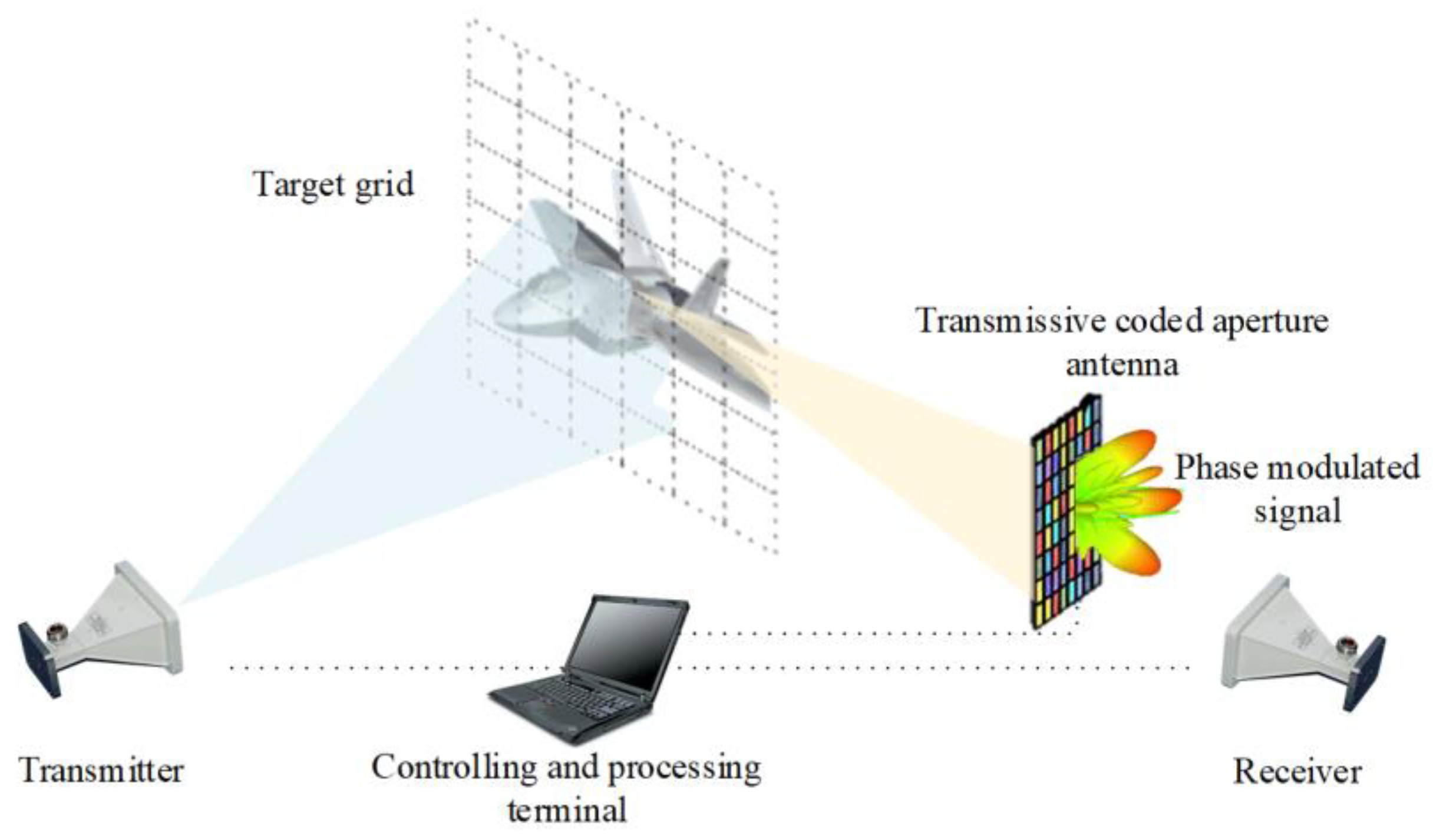
The microwave computational imaging (MCI) system based on transmissive information metamaterials is shown in Figure 1. The MCI system consists of a transmitter and receiver, processor terminal, and a coding aperture antenna at the receiving end that works as phase modulation. The signal reflected from the target can be received by a coded aperture antenna. The 1-bit digitally controlled coded aperture antenna is employed for the quick modulation of the received signal phase. Then, the echo signal is sampled and sent to the processor to reconstruct the target scatterers. The scattered electromagnetic waves are phase modulated by the transmissive aperture coding antenna at the receiving end and finally received by the receiving antenna. The signal processing terminal reconstructs the target through computational imaging.

In the two-dimensional MCI imaging model, we assume that the imaging plane is divided into $W$ grid units, and the strong scatterers of the target are at the center of the grid cells. The number of encoded array elements for information metamaterial antennas is $M$. Assuming that the transmitting signal $s_t(t)$ reaches the target at time $t_n$, the reflected signal at the w-th imaging grid is expressed as follows:

$$s\left(t_n,w\right)=s_t\left(t_n-d_w/c\right).$$

(1)

where $d_w$ denotes the distance from the transmitting antenna to the w-th grid. Then, the reflected signal arriving at the m-th coded-aperture antenna is the sum of the reflected signals from all the imaging plane grids:

$$\begin{array}{c}s\left(t_n,m\right)={\displaystyle \sum _{w=1}^W{A}_m\left(t_n\right)}s\left(t_n-{\displaystyle \frac{d_{m,w}}{c}},w\right)\exp \left(j{\phi }_m\left(t_n\right)\right){\beta }_w\\ =A_m(t_n){\displaystyle \sum _{w=1}^{W}s(t_n-\frac{d_w+d_{m,w}}{c})\exp (j{\phi }_m(t_n))}{\beta }_w.\end{array}$$

(2)

where $A_m\left(t_n\right)$ denotes the amplitude modulation factor of the m-th coding unit at the moment $t_n$, $d_{m,w}$ represents the distance between the m-th coding array element and the w-th imaging grid, and ${\phi }_m\left(t_n\right)$ is the phase modulation factor of the m-th coding unit, ${\beta }_w$ which is expressed as the scattering coefficient of the w-th imaging grid. The echo signal received by the receiving antenna located behind the information metamaterial is a superposition of $M$ modulated signals:

$$\begin{array}{c}Sr\left(t_n\right)={\displaystyle \sum _{m=1}^M{\displaystyle \sum _{w=1}^W{A}_m\left(t_n\right)s}\left(t_n-\frac{d_m}{c},m\right)\exp \left(j{\phi }_m\left(t_n\right)\right)}{\beta }_w\\ =A_m(t_n){\displaystyle \sum _{w=1}^W{s}_t(t_n-\frac{d_w+d_{m,w}+d_m}{c})\exp (j{\phi }_m(t_n))}{\beta }_w.\end{array}$$

(3)

where $d_m$ represents the distance between the m-th metamaterial coding array element and the receiving antenna, and in order to express it in the form of the multiplication of the reference signal with the scattering coefficient, the Equation (3) is rewritten as follows:

$$Sr\left(t_n\right)={\displaystyle \sum _{w=1}^{W}S\left(t_n,w\right)}\cdot {\beta }_w.$$

(4)

where $S\left(t_n,w\right)$ is the reference signal corresponding to the w-th grid cell in the imaging region.

$$S\left(t_n,w\right)={\displaystyle \sum _{m=1}^M{A}_m\left(t_n\right)s_{tr}\left(t_n-\frac{d_w+d_m}{c}\right)}\exp \left(j{\phi }_m\left(t_n\right)\right).$$

(5)

At the signal transmitter end, a single signal is emitted, and the entire process is divided into $N$ time segments. The echo signals received at the receiver end at different time intervals are represented as the following echo signal matrix:

$$\left[\begin{array}{c}Sr\left(t_1\right)\\ Sr\left(t_2\right)\\ ⋮\\ Sr\left(t_n\right)\\ ⋮\\ Sr\left(t_N\right)\end{array}\right]=\left[\begin{array}{cccccc}S\left(t_1,1\right)& S\left(t_1,2\right)& \cdots & S\left(t_1,w\right)& \cdots & S\left(t_1,W\right)\\ S\left(t_2,1\right)& S\left(t_2,2\right)& \cdots & S\left(t_2,w\right)& \cdots & S\left(t_2,W\right)\\ ⋮& ⋮& ⋮& ⋮& ⋮& ⋮\\ S\left(t_n,1\right)& S\left(t_n,2\right)& \cdots & S\left(t_n,w\right)& \cdots & S\left(t_n,W\right)\\ ⋮& ⋮& ⋮& ⋮& ⋮& ⋮\\ S\left(t_N,1\right)& S\left(t_N,2\right)& \cdots & S\left(t_N,w\right)& \cdots & S\left(t_N,W\right)\end{array}\right]\cdot \left[\begin{array}{c}{\beta }_w\\ {\beta }_w\\ ⋮\\ {\beta }_w\\ ⋮\\ {\beta }_w\end{array}\right]+\left[\begin{array}{c}{\omega }_1\\ {\omega }_2\\ ⋮\\ {\omega }_n\\ ⋮\\ {\omega }_N\end{array}\right].$$

(6)

where ${\omega }_N$ denotes the measurement noise at the nth coded measurement receive echo reception, and $N$ is the number of coded measurement patterns. The form of the matrix equation expressed in Equation (6) can also be written in the form of a vector matrix:

$$Sr=S\cdot \mathbf{\beta }+\mathbf{\omega }.$$

(7)

Equation (7) is the sensing model of the system. Where $Sr\in C^{N\times 1}$ is the vector of echo signals throughout the $N$ measurements. $S\in C^{N\times W}$ represents the reference signal matrix, also known as the sensing matrix, whose correlation is determined by the coding mode of the coded aperture. $\mathbf{\beta }\in C^{W\times 1}$ is the vector of scattering coefficients corresponding to the center of the grid cell of the imaging region, and $\mathbf{\omega }\in C^{W\times 1}$ denotes the noise vector.

The compression ratio is the ratio of the number of measured codes to the number of image grids, as follows:

$$\gamma =N/W.$$

(8)

From the imaging modeling process, it can be seen that the solution of the scattering coefficients mainly relies on the row-to-row and column-to-column correlations of the reference signal matrix. The stronger the modulation capability of the coded antenna, the stronger the non-correlation of S, and the more accurate the solution of the target scattering coefficient.

The sparsity criterion of the target is measured by the relationship between the L1 and L2 norms of a given vector [34].

$$Sparsness\left(\beta \right)=\sqrt{N}-{\displaystyle \frac{\sum \left|{\beta }_i\right|}{\sqrt{\sum |{\beta }_i{|}^2}}}/\sqrt{N}-1.$$

(9)

where $\beta$ denotes the scattering coefficient of the imaging target, N is the pixel of the imaging target, and the influence of image sparsity on the reconstructed image is very important. A high sparsity image means that there are many zero pixels in the image, and in image reconstruction, a high sparsity image can often be better reconstructed. This is because images with high sparsity have fewer non-zero pixels, which can be reduced in storage space and computational complexity through compression and sparse representation methods.

3. Method

In order to improve the quality of target reconstruction, Existing methods mainly focus on two aspects [36,37]: the design of encoding modes in the measurement phase and the design of computational algorithms in the reconstruction phase, which are also referred to as microwave encoders and computational decoder design.

In previous studies, when employing 1-bit information metamaterial antennas, the random matrix with equal 0/1 probabilities (p = 0.5) demonstrated superior robustness in most scenarios. Consequently, the majority of coding pattern selections were either directly based on random matrices for aperture coding imaging or involved the optimization of coding matrices.

In the reconstruction stage, most methods are based on optimization problems, utilizing compressed sensing theory and prior information to adjust the loss function through regularization, such as Tikhonov regularization [38], Orthogonal Matching Pursuit (OMP) [39], Total Variation Augmented Lagrangian Alternating Direction Algorithm [40], and CNN [41]. However, existing methods often overlook the link between these two phases, typically considering them separately, which limits the improvement of imaging quality.

In the field of optics, data-driven deep learning methods leverage an increasing number of datasets to learn non-linear transformations, mapping projected encoded measurements to the desired output. This enables direct target reconstruction from projected encoded measurements by easily altering the deep neural network architecture and loss function. The use of a large number of data-driven methods to design encoding apertures means that the design of microwave encoders and computational decoders can be synchronized, achieving the joint optimization of both.

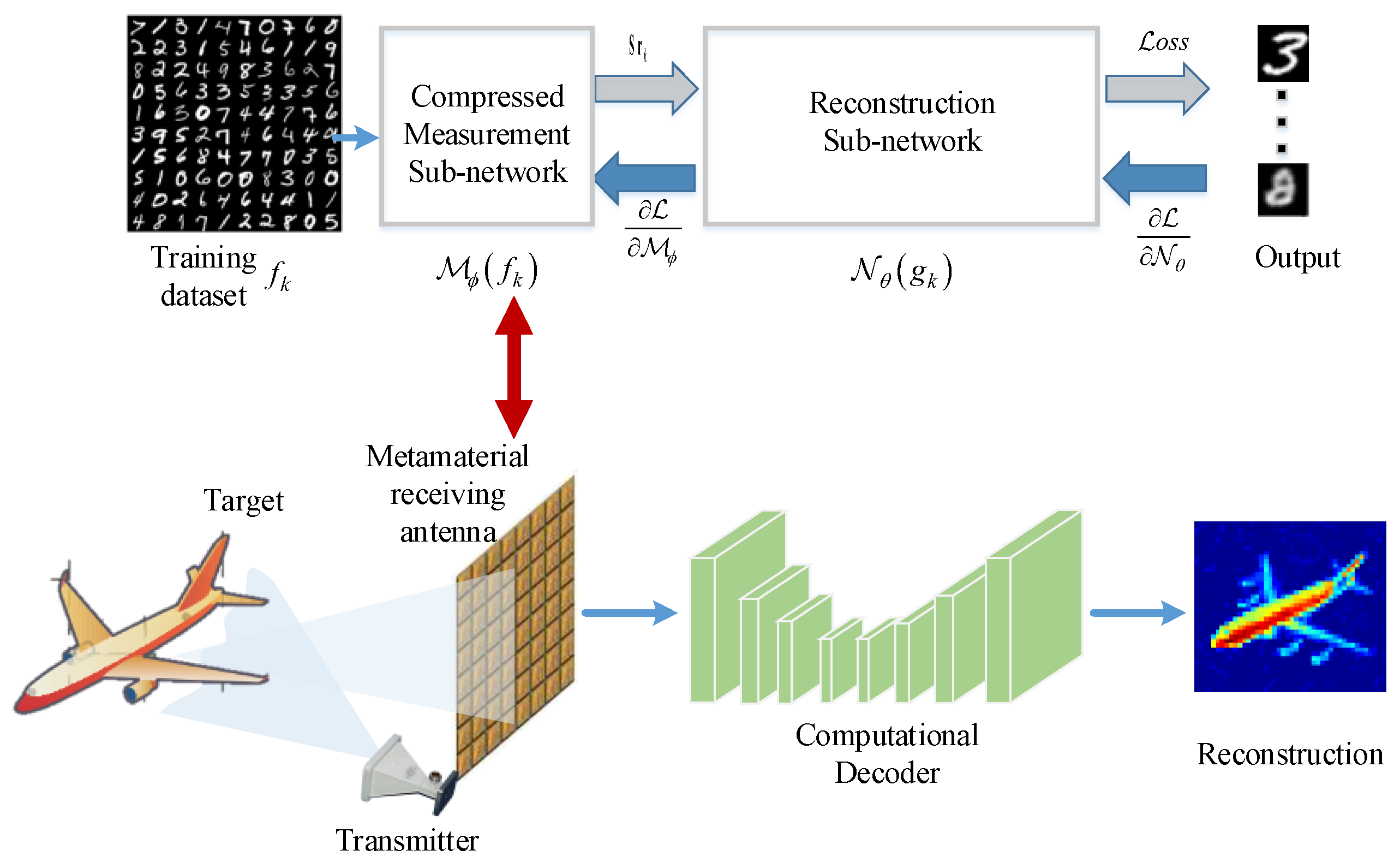
The microwave computational imaging system consists of two stages: the measurement stage and the reconstruction stage. In the proposed end-to-end framework, these two stages are integrated into a unified network, as illustrated in Figure 2.

In MCI based on information metamaterials, the metamaterial antenna updates the encoding and modulates the echo phase each time the target is measured. Although the reference matrix $\mathbf{S}$ is determined by the encoding mode of the metamaterial antenna, inferring the encoding mode from the known reference matrix $\mathbf{S}$ is difficult. Therefore, it is not feasible to directly parameterize the reference matrix into convolutional layers to simulate the measurement process of the system. In order to directly represent the encoding mode of metamaterial antennas as convolutional layers, the reference matrix is rewritten as follows:

$$\mathbf{S}=\mathbf{D}\mathbf{B}.$$

(10)

The dimensions of each matrix in the equation are $\mathbf{D}\in Z^{N\times M}$, $\mathbf{B}\in C^{M\times W}$. The composition of matrix D is as follows:

$$\mathbf{D}=\left[\begin{array}{ccccc}\exp \left(j{\phi }_1\left(t_1\right)\right)& \cdots & \exp \left(j{\phi }_m\left(t_1\right)\right)& \cdots & \exp \left(j{\phi }_M\left(t_1\right)\right)\\ \exp \left(j{\phi }_1\left(t_2\right)\right)& \cdots & \exp \left(j{\phi }_m\left(t_2\right)\right)& \cdots & \exp \left(j{\phi }_M\left(t_2\right)\right)\\ ⋮& ⋮& ⋮& ⋮& ⋮\\ \exp \left(j{\phi }_1\left(t_n\right)\right)& \cdots & \exp \left(j{\phi }_m\left(t_n\right)\right)& \cdots & \exp \left(j{\phi }_M\left(t_n\right)\right)\\ ⋮& ⋮& ⋮& ⋮& ⋮\\ \exp \left(j{\phi }_1\left(t_N\right)\right)& \cdots & \exp \left(j{\phi }_m\left(t_N\right)\right)& \cdots & \exp \left(j{\phi }_M\left(t_N\right)\right)\end{array}\right].$$

(11)

Each of its rows represents the coding pattern of the informative metamaterial antenna in a particular measurement, and the elements of the matrix D consist of 1 or −1 since the modulation phase of the metamaterial antenna array elements is 0 or π. The elements of the coding matrix D are completely determined by the coding pattern of the metamaterial antenna, and thus, the matrix is referred to as the coding pattern matrix.

The construction method of matrix B is as follows:

$$\mathbf{B}=\left[\begin{array}{cccccc}{S}^{\prime }\left(t_1,1,1\right)& S^{\prime }\left(t_2,1,2\right)& \cdots & S^{\prime }\left(t_n,1,w\right)& \cdots & S^{\prime }\left(t_N,1,W\right)\\ S^{\prime }\left(t_1,2,1\right)& S^{\prime }\left(t_2,2,2\right)& \cdots & S\left(t_n,2,w\right)& \cdots & S^{\prime }\left(t_N,2,W\right)\\ ⋮& ⋮& ⋮& ⋮& ⋮& ⋮\\ S^{\prime }\left(t_1,m,1\right)& S^{\prime }\left(t_2,m,2\right)& \cdots & S^{\prime }\left(t_n,m,w\right)& \cdots & S^{\prime }\left(t_N,m,W\right)\\ ⋮& ⋮& ⋮& ⋮& ⋮& ⋮\\ S^{\prime }\left(t_1,M,1\right)& S^{\prime }\left(t_2,M,2\right)& \cdots & S\left(t_n,M,w\right)& \cdots & S\left(t_N,M,W\right)\end{array}\right],$$

(12)

$$S\left(t_n,w\right)={\displaystyle \sum _{m=1}^{M}S\prime \left(t_n,m,w\right)}\cdot \exp (j{\phi }_m(t_{mn})).$$

(13)

Each column of matrix $\mathbf{B}$ represents the unmodulated reference signal corresponding to the wth imaging grid, and its elements are determined by the intrinsic parameters of the MCI-based information metamaterial aperture system, such as the imaging distance of the system, the number of array elements of the informative metamaterial antenna, and the radar signal parameters. Therefore, $\mathbf{B}$ is referred to as the system matrix.

As shown in Figure 3a, the following section provides a detailed explanation of the four parts of an end-to-end network.

Pretreatment: As expressed in Equation (10), the reference matrix has been represented in the form of the product between the coding matrix D and the system matrix B. Now, the sensing matrix of the system is transformed into the following form:

$$\mathbf{S}\mathbf{r}=\mathbf{S}\mathit{\beta }=\mathbf{D}\mathbf{B}\mathit{\beta }=\mathbf{D}\mathit{\beta }\mathbf{\prime }.$$

(14)

The dimensions of the matrices in Equation (14) are $\mathit{\beta }\mathbf{\prime }\in C^{M\times 1}$. The transformation of the aforementioned sensing model is facilitated by the fact that matrix B is a constant matrix—once the parameters of the imaging system are fixed, B remains invariant. The transformation process of $\mathit{\beta }\mathbf{\prime }=\mathit{B}\mathit{\beta }$ is called preprocessing.

Compressed measurement subnetwork: to simulate the measurement process using a convolutional layer, based on the sensing model $\mathbf{S}\mathbf{r}=\mathbf{D}\mathit{\beta }\mathbf{\prime }$, the $N$ $N$ rows of the coding pattern of the matrix D in Equation (14) are considered as $N$ filters, each of size $1\times 1\times M$. The echo vector is the result of filtering vector $\mathit{\beta }\mathbf{\prime }$ $N$ times. Thus, the measurement process can be modeled as a convolutional layer with $N$ filters, and since it is non-overlapping sampling, the step size of the convolutional layer is set to 1 × 1, and its input is a vector of length $M$, and its output is a vector of length $N$. The elements of the coding pattern matrix D correspond to each other and can be automatically updated for optimization in the network. Since the matrix D is a binary matrix consisting of 1 or −1, constraints need to be added so that the weights of the convolutional layer after training are {1, −1}. After training, the weights of this layer are the optimized coding pattern, which can be used to replace the random coding pattern in subsequent measurements, thus obtaining better reconstruction results.

Initial reconstruction subnetwork: For the initial reconstructed image, the common method is usually to calculate the pseudo inverse matrix of the reference matrix.

$$x=\mathrm{pinv}\left(\mathbf{S}\right)\cdot \mathbf{S}\mathbf{r}.$$

(15)

where pinv denotes the pseudo-inverse matrix operator and the dimension of the pseudo-inverse matrix is $\mathrm{pinv}\left(\mathbf{S}\right)\in C^{W\times N}$, $x$$\in C^{W\times 1}$ denotes the initial reconstructed image, and $\mathbf{S}\mathbf{r}\in C^{N\times 1}$ is the echo vector, with each element being a complex number. In order to transform the above initial image reconstruction process into a convolutional layer form, similar to the measurement subnetwork in the previous section, we use a convolutional layer with $W$ filters to express the initial image reconstruction process, where each filter is of size $1\times 1\times N$.

Since the output of the measurement subnetwork is an $N\times 1$ complex vector, the two column vectors of the real and imaginary parts of Sr are taken as inputs to the initial reconstruction subnetwork, which outputs two vectors of length W. In order to transform the output vectors into an initial image, a shaping operation is added to the back-end of the convolutional layer. This operation can reconstruct the vector of $1\times W$ dimension into an initial image matrix of $\sqrt{W}\times \sqrt{W}$ dimension, and then input it into the deep reconstruction subnetwork of the backend for further reconstruction.

The image generated by the initial reconstruction subnetwork is still defocused. Therefore, in order to obtain high-resolution imaging results, this paper applies U-Net to achieve an accurate reconstruction of the target, and the network structure is shown in Figure 3b [41]. The proposed reconstruction network is based on a U-Net-style encoder-decoder architecture. It mainly consists of an encoder, decoder, and skip connection. The encoder first performs convolution and pooling operations on the input image, gradually reducing the size of the image and increasing the number of channels, in order to extract the features of the image, and uses a linear rectification function $\mathrm{Relu}\left(x\right)=\max \left\{0,x\right\}$ as the activation function. The decoder fuses the extracted features through upsampling and convolutional layers and achieves the transformation from the feature domain to the image domain. The input is a complex-valued image with size $32\times 32\times 2$, representing the real and imaginary components. The encoder includes four convolutional layers (kernel size $3\times 3$) with ReLU activation, interleaved with max-pooling layers (stride 2). The decoder uses transposed convolutions ($2\times 2$) and skip connections to restore spatial resolution. The final output layer is a single-channel $32\times 32\times 1$ image passed through a Sigmoid activation. Training is performed using the Adam optimizer with a learning rate of 1 × 10⁻⁴, batch size of 32, for 200 epochs. The U-Net network can effectively process microwave images containing noise or incomplete data. The skip connections in the network preserve high-resolution features and enhance imaging details.

The convolutional layer in the constructed compressive measurement subnetwork can automatically learn the optimal coding patterns, but the learned weights are floating point numbers without constraints, which is difficult to achieve in practical applications. Therefore, some constraints need to be imposed on the optimization process to ensure that the learned coding patterns are binary. To this end, we introduce a binary regularizer in the loss function to implement the constraints, as shown in the following equation:

$$R_{\rho }\left(\mathit{\varphi }\right)={\displaystyle \frac{1}{M}}{\displaystyle \sum }_{m=1}^M{\left({\mathit{\varphi }}_m+1\right)}^2{\left({\mathit{\varphi }}_m-1\right)}^2.$$

(16)

In Equation (16), $\varphi$ denotes the coded aperture pattern and $M$ denotes the number of coding units of the metamaterial antenna. It can be seen that when the $\mathit{\varphi }$ term is taken as 1 or −1, the minimum value of $R_{\rho }$($\mathit{\varphi }$) can be obtained. It is formulated as a continuous approximation of the sign function, commonly used in binary neural networks, and pushes the learned patterns toward the desired discrete values {−1, 1}. This helps match the physical constraint of 1-bit programmable metasurfaces, which support only two phase states (0 and π).

In the MCI system, the more uncorrelated the random radiation field generated by the metamaterial antenna in time, the better the imaging results will be. The non-coherence of the radiation field in the time dimension is achieved by changing the encoding mode. Therefore, a regularization function is designed as follows to reduce the correlation between each encoding mode:

$$R_{\sigma }\left(\mathit{\varphi }\right)={\displaystyle \frac{1}{M}}{\displaystyle \sum }_{m=1}^M\left({\displaystyle \prod }_{n=1}^N{\mathit{\varphi }}_m^n\right).$$

(17)

In Equation (17), $N$ represents the number of encoding measurements and ${\mathit{\varphi }}_m^n$ represents the value of the m-th encoding unit during the nth measurement. The weaker the correlation of $N$ encoding measurement modes, the smaller the $R_{\rho }$($\mathit{\varphi }$). $R_{\sigma }$($\mathit{\varphi }$) penalizes the mutual correlation among different encoding patterns. Specifically, it minimizes the off-diagonal Frobenius norm of the Gram matrix formed by the rows of the encoding matrix. This design is inspired by compressed sensing theory, in which lower mutual coherence leads to better signal recovery. Therefore, the regularization term is added to the loss function to reduce the correlation between each encoding mode.

The imaging process of MCI is expressed as an end-to-end network that directly learns an end-to-end mapping between the compression measurements and the target image. The input and labels during training of this network are the target images themselves. Similar to deep neural networks used for image restoration, we use the mean square error (MSE) as the loss function of the proposed end-to-end network, and its training process can be interpreted as the following loss function optimization problem:

$$\left\{{\mathit{\varphi }}^{*},{\theta }^{*}\right\}\in \underset{\mathit{\varphi },\theta }{{\displaystyle argmin}} L\left(\mathit{\varphi },\theta \right),$$

(18)

$$L(\varphi ,\theta )={\displaystyle \frac{1}{K}}{\displaystyle \sum _{k=1}^K{‖N_{\theta }(M_{\varphi }(f_k))-f_k‖}^2}+\rho R_{\rho }(\varphi )+\sigma R_{\sigma }(\theta ).$$

(19)

where $\mathit{\varphi }$ represents the weight of the compressed measurement subnetwork, i.e., the coded aperture pattern, $\theta$ represents the weight of the reconstruction network, $\mathit{\varphi }$^* and ${\theta }^{*}$ denote the optimal weights, $M_{\varphi }$ represents the compressed sampling network, $N_{\theta }$ represents the reconstruction network, and ${\left\{f_k\right\}}_{k=1}^K$ represents the training data. $R_{\rho }(\varphi )$ and $R_{\sigma }(\theta )$ denote two regularizers, $R_{\sigma }(\theta )$ serves to suppress the overfitting phenomenon during the training process, $R_{\rho }(\varphi )$ is different from $R_{\sigma }(\theta )$, which serves to impose constraints on the coding aperture patterns, such that the coding patterns must be binary or the correlation between different coding patterns is as small as possible, etc. $\rho$ and $\sigma$ are the regularization parameters of the two regularizers. Adaptive moment estimation is used as an optimizer of the network parameters during training.

In the training stage, each image is treated as an imaging scene, and the original target image is preprocessed to obtain the processed scattering coefficient matrix $\mathit{\beta }\mathit{\prime }$. The $N$ line encoding mode of matrix D in the compressed measurement subnet is equivalent to $N$ filters, and the scattering coefficient matrix $\mathit{\beta }\mathit{\prime }$ is filtered $N$ times by the compressed measurement subnet to obtain the target vector Sr. The binary constraint $R_{\rho }(\varphi )$ and correlation constraint $R_{\sigma }(\theta )$ are added to the compressed measurement subnet. $R_{\rho }(\varphi )$ can convert the learned encoding patterns into binary form, while $R_{\sigma }(\theta )$ reduces the correlation between encoding patterns. In the reconstruction subnetwork, the echo vector Sr obtained from the measurement subnetwork is convolved and shaped to obtain the initial image matrix of $\sqrt{N}\times \sqrt{N}$. Then, it is fed into the u-net network to obtain the final output image. The mean square error is set as the loss function, and the derivatives $\partial L/\partial N_{\theta }$ and $\partial L/\partial M_{\varphi }$ of the backpropagation loss function are used to calculate the minimum loss function during the training process. After updating and optimizing, the weight of matrix D is obtained, which is the optimal encoding mode.

After the training is completed, we used the optimal encoding mode as the optimized aperture encoding mode. At this point, the signal before phase modulation of the input metasurface antenna was inputted, and after optimization, the aperture coding modulation and decoder demodulation were used to obtain the reconstructed image at the output end. The entire process is shown in Figure 4.

4. Experiments

The system parameters are shown in

Table 1. System parameters.

Parameters	Quantity
Centre frequency	15 GHz
Bandwidth	1 GHz
Pulse width	100 ns
Tuning frequency	1016 Hz/s
Imaging distance	6 m
Coding aperture size	0.5 m × 0.5 m
Number of metamaterial cells	41 × 41
Imaging grid size	0.02 m × 0.02 m
Number of imaging grids	32 × 32

. In the simulation, the MNIST [42] and airplane datasets were selected as the target training datasets. The choice of MNIST in our work is motivated by its wide adoption as a benchmark in computational imaging and inverse problem research. It offers a controlled and well-characterized setting that enables the reproducible evaluation of algorithmic performance, especially in the early stages of model development. The aircraft dataset, on the other hand, introduces shape-level complexity and serves as a bridge between abstract digits and structured man-made targets. The dataset consists of 60,000 training images and 20,000 test images, with each dataset representing half of the total. These datasets represent the imaging targets in the microwave imaging system. The target dimensions are standardized at 32 × 32 pixels, with each image comprising an identical number of scattering points. Consistent with radar target characteristics, the scattering point values are normalized to random values within the range [0, 1], which subsequently serve as both the input and labels for the end-to-end network. We use the U-NET convolutional neural network to process the datasets. The initial learning rate is set to 10⁻⁴, and the code is implemented in TensorFlow. The neural network is trained on a desktop computer with an NVIDIA 2080 GPU and CUDA version 10.0.

In order to verify the performance of the proposed method, it was compared with several commonly used competitive algorithms. Specifically, commonly used computational imaging reconstruction algorithms include the OMP algorithm, sparse Bayesian learning (SBL) algorithm, and the alternative direction multiplier method (ADMM). The method of using random coded aperture and only using deep neural networks for recovery tasks is called Random-CA, and the method used in this article is called learning CA.

All other algorithms compared to end-to-end methods use random encoded aperture patterns. To quantitatively measure the performance of different algorithms, this paper evaluates the reconstruction quality by calculating three quantitative image quality indicators, including relative error (RE), peak signal-to-noise ratio (PSNR), and structural similarity index measure (SSIM). The smaller the value of RE, the higher the values of PSNR and SSIM, indicating a better reconstruction quality of the target image.

$$\mathrm{RE}={\displaystyle \frac{{‖\widehat{\mathbf{x}}-\mathbf{x}‖}_2^2}{{‖\mathbf{x}‖}_2^2}}.$$

(20)

In Equation (20), $\widehat{\mathbf{x}}$ and $\mathbf{x}$ represent the original signal and the recovered signal, respectively.

$$\mathrm{PSNR}=10{\log }_{10}({\displaystyle \frac{{\mathrm{Max}}^2}{\mathrm{MSE}}}).$$

(21)

In Equation (21), $\mathrm{Max}$ is the maximum pixel value of the original image, MSE is the mean square error.

$$\mathrm{SSIM}(\mathrm{x},\mathrm{h})=\mathrm{l}{(\mathrm{x},\mathrm{h})}^{\alpha }\mathrm{c}{(\mathrm{x},\mathrm{h})}^{\chi }\mathrm{s}{(\mathrm{x},\mathrm{h})}^{\epsilon }.$$

(22)

In Equation (22), $\mathrm{x}$ and $\mathrm{h}$ are the pixel values of the original and reconstructed images, respectively, $\mathrm{l},\mathrm{c},\mathrm{s}$ are the brightness, contrast, and structure functions, respectively, and $\alpha ,\chi ,\epsilon$ are the weights.

4.1. Reconstruction Results of Targets with Different Sparsity

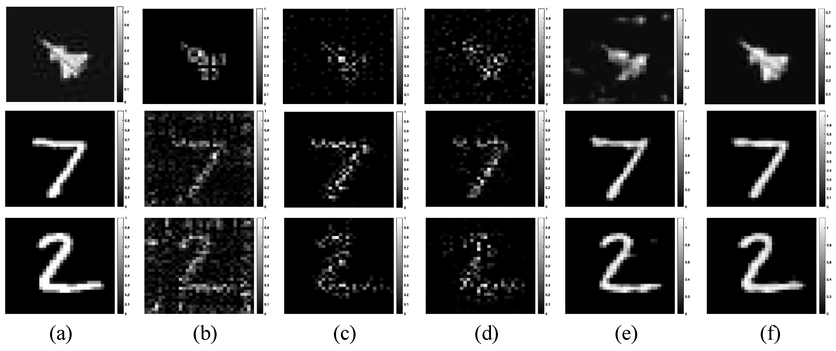
Consider imaging tasks on targets with different sparsity. Figure 5 shows the results of reconstructing different sparsity targets using multiple algorithms. The original target images are number 7, number 2, and aircraft, with sparsities of 0.7288, 0.6620, and 0.4320, respectively. We set the SNR to 20 dB and the compression ratio to 0.5. The quantitative analysis of imaging quality is shown in

Table 2. Imaging results for different methods. The best results are in bold.

Metrics	PSNR(dB)	RE	SSIM
OMP	10.79	0.0839	0.1807
ADMM	10.91	0.0811	0.0051
SBL	11.19	0.0759	0.1697
TVAL3	19.86	0.0211	0.814
Random-CA	20.16	0.0110	0.828
Learned-CA	25.86	0.0030	0.953

. On the one hand, it can be seen that the proposed method can successfully reconstruct the target and is superior to typical computational imaging reconstruction algorithms. On the other hand, compared with random CA, this method also achieves better reconstruction results, proving the effectiveness of the deep coding aperture pattern optimization proposed in this paper.

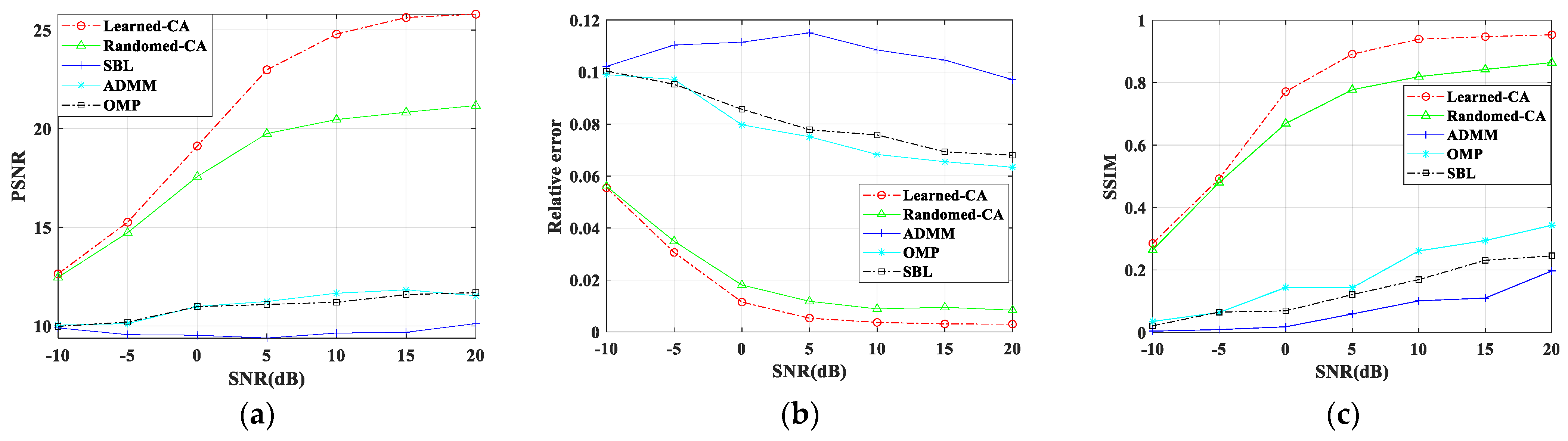
4.2. Noise Robustness

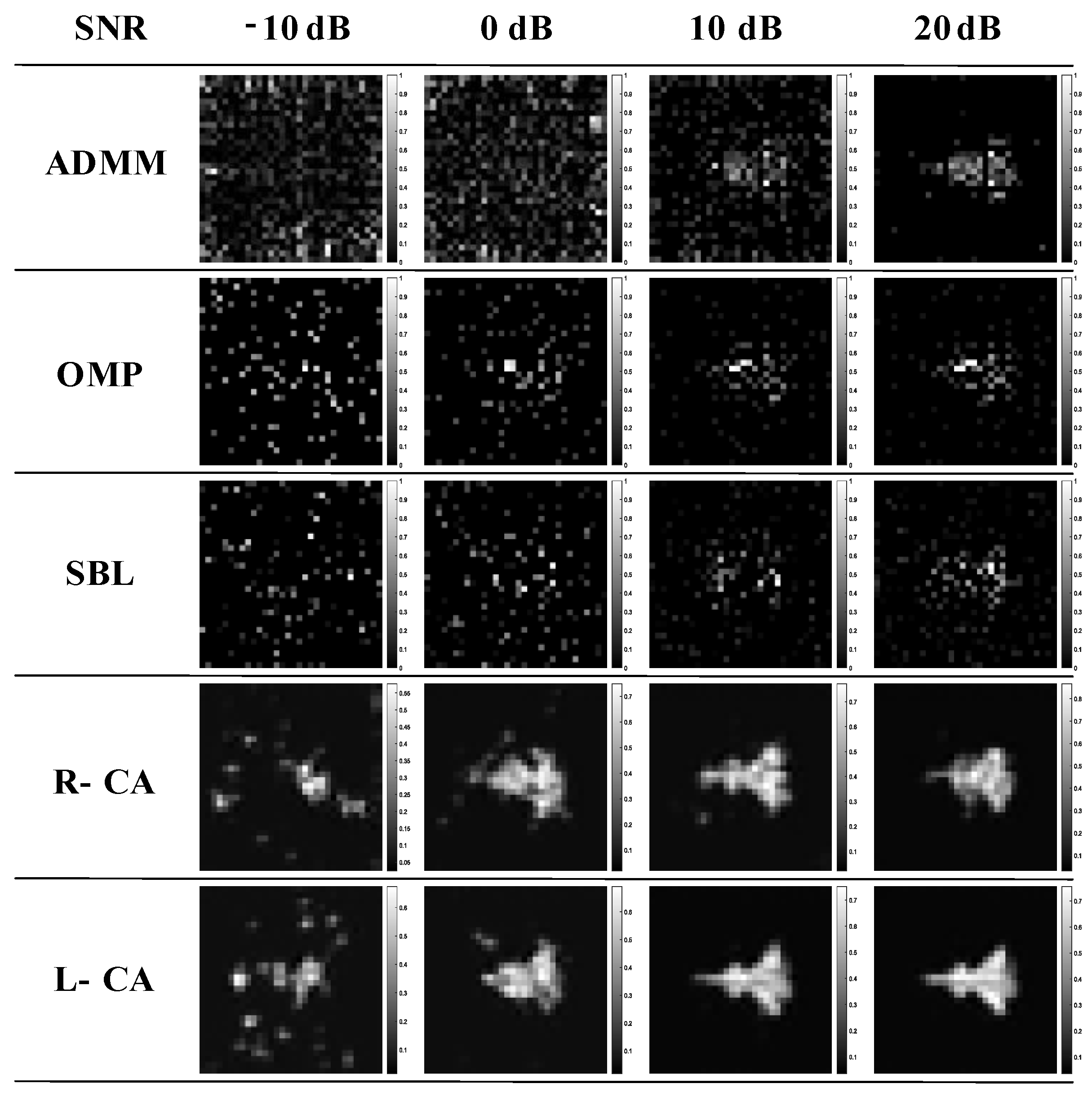
In the simulation experiment, we used the MNIST dataset and aircraft image dataset, with the original target compression ratio set to 0.5, and added Gaussian white noise with different SNR to the echo for imaging. We compared this method with four algorithms to visually observe and quantitatively analyze imaging quality. Figure 6 shows the imaging results under different SNR, and Figure 7 shows the quantitative analysis line chart of three measurements. From the comparison of imaging results and imaging performance, it can be seen that the method proposed in this paper has good noise robustness.

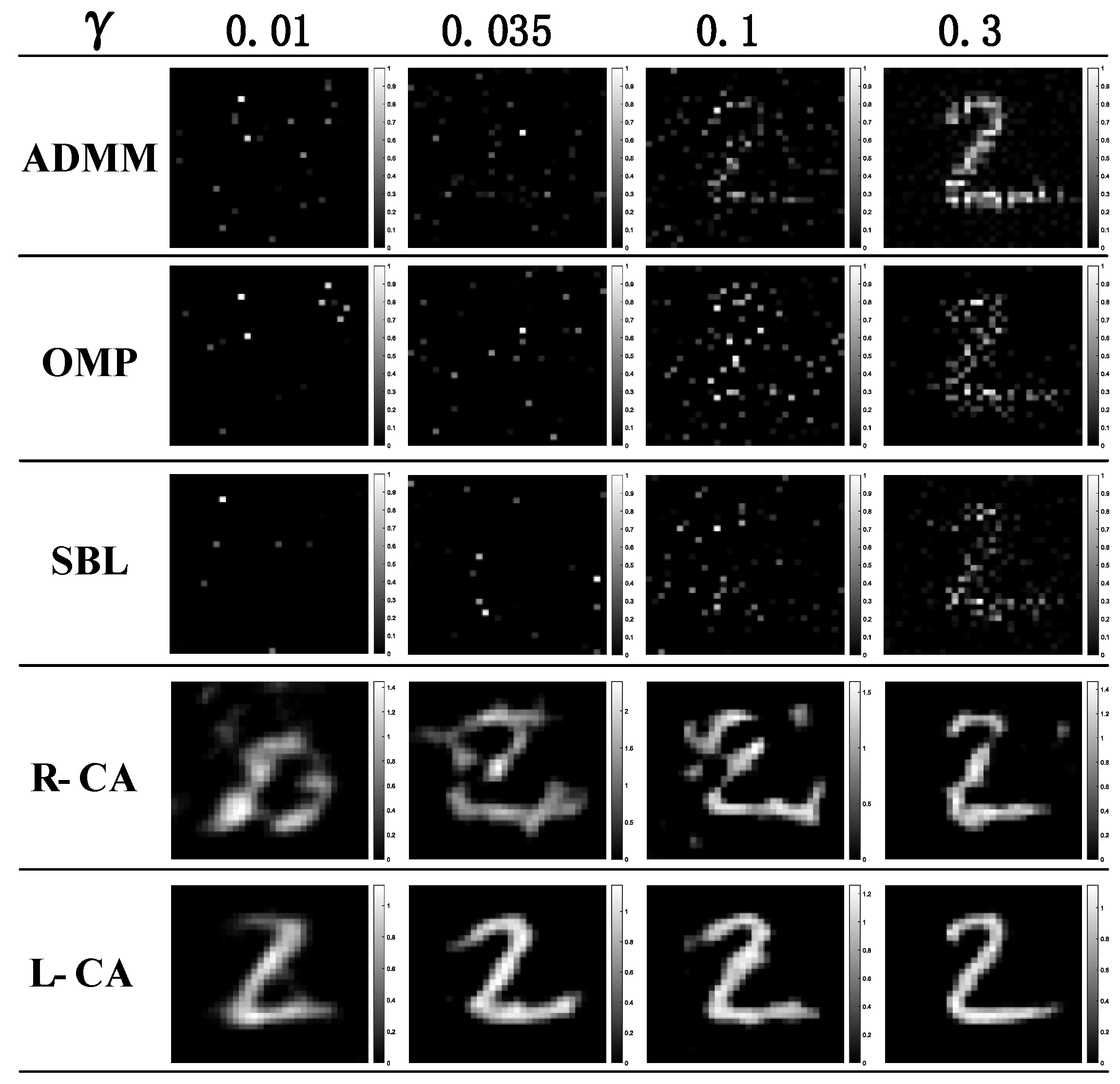
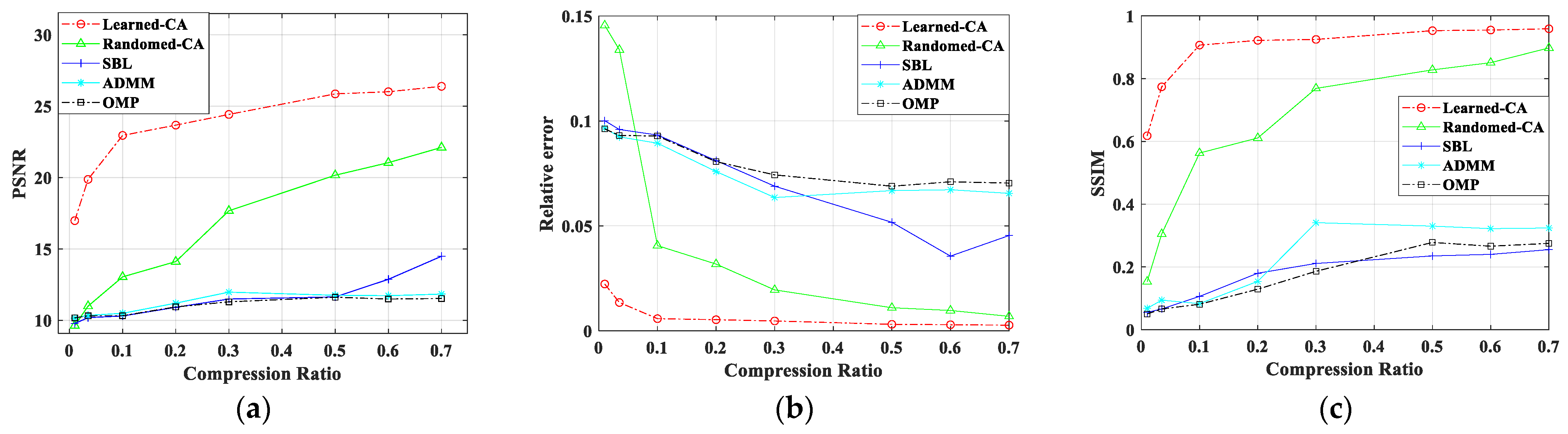
4.3. Reconstruction Results of Targets with Different Compression Ratio Measurements

In order to investigate the reconstruction performance of the proposed method under compression measurements, the echo signal was imaged with a SNR of 20 dB, and handwritten digital targets were imaged under different compression ratios. The imaging results under different compression ratio measurements are given in Figure 8, and Figure 9 shows the line graphs of quantitative imaging performance metrics under different compression ratios. It can be seen that the method in this paper significantly improves the recoverable compression ratio, i.e., the measurement pattern is limited, the target is sparsely sampled, the proposed method can still perform the recovery task when other algorithms are unable to reconstruct the target image under low compression ratios, and better performance can be obtained when the target is measured using the coded aperture learnt from the end-to-end network.

To assess the stability and reliability of our proposed Learned-CA method across various experimental conditions, we performed 50 independent Monte Carlo simulations for each predefined compression ratio. The 95% confidence intervals were computed using the statistical formula $C{I}_{95\%}=\overline{x}\pm s/\sqrt{n}$ based on the standard deviation of experimental results from each group (where $\overline{x}$ is the sample mean, $s$ is the standard deviation, n = 50), thereby demonstrating the method’s statistical stability and confidence level.

An observation of

Table 3. The confidence intervals of PSNR for our proposed algorithm.

	Mean PSNR(dB)	95% CI Lower	95% CI Upper
0.01	16.33	16.27	16.39
0.1	23.51	23.47	23.55
0.2	24.28	24.24	24.32
0.3	24.67	24.63	24.71
0.4	25.03	24.97	25.09
0.5	25.94	24.89	24.99
0.6	26.05	26.01	26.09
0.7	26.32	26.49	26.35

,

Table 4. The confidence intervals of RE for our proposed algorithm.

	Mean RE	95% CI Lower	95% CI Upper
0.01	0.0359	0.0345	0.0373
0.1	0.0134	0.012	0.0148
0.2	0.0112	0.0099	0.0125
0.3	0.0098	0.0083	0.0113
0.4	0.0084	0.0072	0.0096
0.5	0.0075	0.0063	0.0087
0.6	0.0071	0.0058	0.0084
0.7	0.0058	0.0046	0.006

and

Table 5. The confidence intervals of SSIM for our proposed algorithm.

	Mean SSIM	95% CI Lower	95% CI Upper
0.01	0.6113	0.6032	0.6194
0.1	0.9211	0.9138	0.9284
0.2	0.9227	0.9167	0.9287
0.3	0.9246	0.9183	0.9309
0.4	0.9305	0.937	0.924
0.5	0.9342	0.9292	0.9392
0.6	0.9381	0.9333	0.9429
0.7	0.9404	0.9369	0.9439

reveals that the proposed algorithm consistently maintains tight confidence intervals across various experimental settings, which reflects its robustness and the statistical stability of its performance.

4.4. Computational Complexity and Inference Efficiency

To assess the practicality of the proposed method in real-world applications, especially under real-time or resource-constrained scenarios, we present a comprehensive analysis of the computational complexity, inference speed, and memory usage of our deep learning-based reconstruction framework. A comparative evaluation against conventional iterative methods, including ADMM, OMP, and SBL, is also provided.

The inference process of our model consists of a fixed number of convolutional and linear operations, resulting in a theoretical computational complexity of $O(n^2)$, where n denotes the image dimension. In contrast, traditional iterative methods involve multiple matrix multiplications, sparse recovery, and inversion operations, leading to higher computational burdens—typically exceeding $O(n^3)$ over several iterations. We benchmarked all methods on an NVIDIA RTX 2080 GPU(NVIDIA, Santa Clara, CA, USA) using 32 × 32 input images at a compression ratio of $\gamma =0.3$. As shown in

Table 6. The complexity analysis of our proposed algorithm.

Method	Inference Time (ms)	FLOPs (×106)	GPU Memory Usage (MB)
ADMM	470	920	1200
OMP	320	750	960
SBL	280	680	900
Randomed-CA	30	85	490
Learned-CA	28	85	480

, the proposed method achieved an inference time of 28 ms and GPU memory usage of approximately 480 MB, which is significantly lower than ADMM (470 ms, 1200 MB) and OMP (320 ms, 960 MB). In terms of FLOPs, the proposed network requires ~85 M floating-point operations, compared to 920 M for ADMM and 750 M for OMP, confirming its computational efficiency. Moreover, since the architecture remains fixed across varying SNR levels and compression ratios, the inference cost does not increase under more challenging conditions, unlike iterative methods, whose performance and convergence are highly sensitive to γ and noise levels.

5. Conclusions

This paper focuses on the optimization of encoding aperture in MCI systems. We have designed a microwave computational imaging method based on information metamaterials and end-to-end deep learning, for the joint optimization of coding aperture design and computational imaging methods in MCI systems. This method converts the encoding aperture of the end-to-end network into a weight layer for optimization. To make the optimized encoding aperture physically achievable, multiple regularization functions are used to implement constraints. Compared with existing computational imaging algorithms, this paper combines encoding aperture design and computational imaging into end-to-end networks and trains them to obtain the optimal encoding method. This network has certain advantages over classical imaging algorithms in reconstructing targets with different sparsity at low SNR. This system can reconstruct high-resolution sparse targets under compressed measurement, with good noise resistance and an improved recoverable compression ratio.

Future Work

To further enhance the applicability and practicality of the proposed method, several future research directions are worth pursuing.

First, although the current study validates the effectiveness of our approach through numerical simulations, real-world implementation remains a critical next step. We plan to construct a small-scale experimental prototype using 1-bit programmable metamaterials based on PIN diode or MEMS technology. This prototype will allow us to assess the feasibility of deploying the learned encoding patterns in physical systems and to examine the system’s robustness under hardware non-idealities, such as phase deviation, switching delay, and electromagnetic interference. Second, the scalability of the proposed framework is an important concern. While the model performs well on 32 × 32 resolution images, we encountered GPU memory overflow during training on higher-resolution data (e.g., 128 × 128). To overcome this limitation, we will explore modular decoupling strategies—such as stage-wise training—where the reconstruction network is pre-trained and the encoding pattern is subsequently optimized—as well as patch-wise processing and lightweight network design. These approaches are expected to improve the model’s efficiency and scalability. Third, the manufacturability of the optimized binary encoding patterns will be systematically studied. Although current programmable metamaterials support binary phase modulation, fabrication tolerances and imperfect switching may introduce deviations from the ideal {−1, 1} values. To mitigate this, we incorporated binary constraints and correlation-penalizing regularization during training to enhance pattern robustness. Future work will also consider quantization-aware training and hardware-in-the-loop simulations to better align the learned encoding patterns with real-world hardware characteristics.

Through these efforts, we aim to bridge the gap between algorithm design and physical implementation, advancing toward practical, real-time, high-resolution microwave computational imaging systems.