
Depth Upsampling with Local and Nonlocal Models Using Adaptive Bandwidth

Abstract
1. Introduction
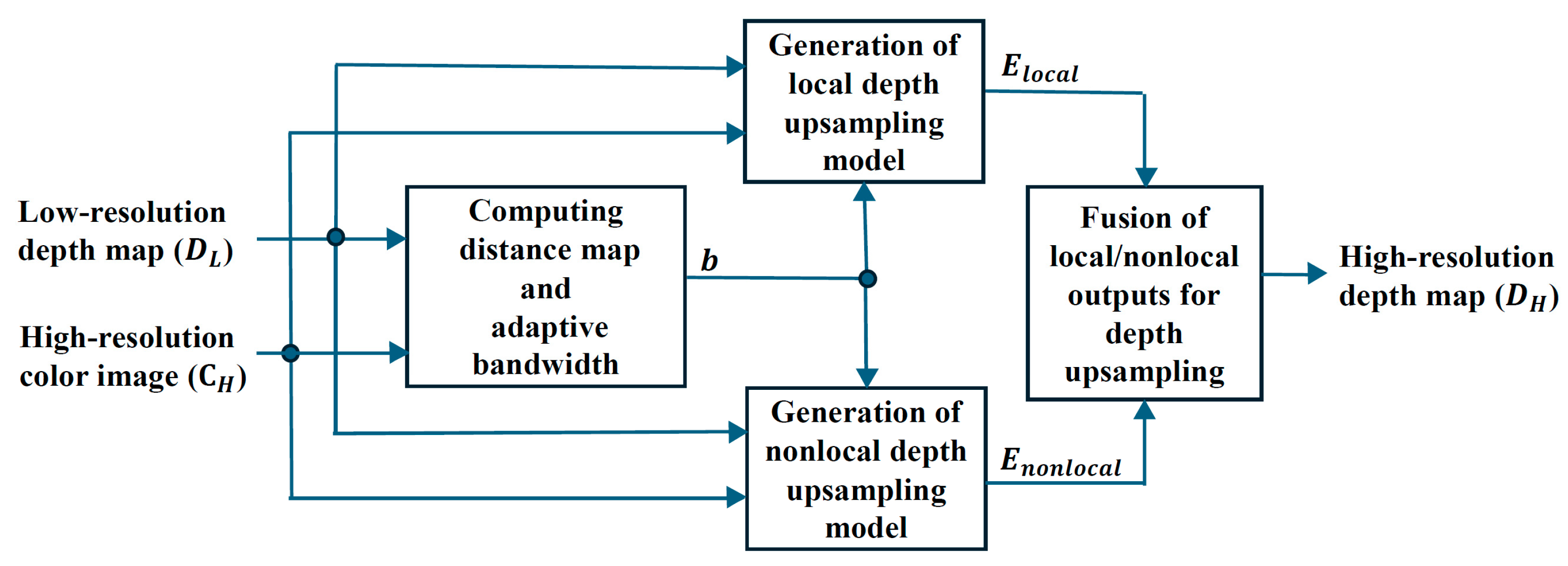
2. Proposed Method
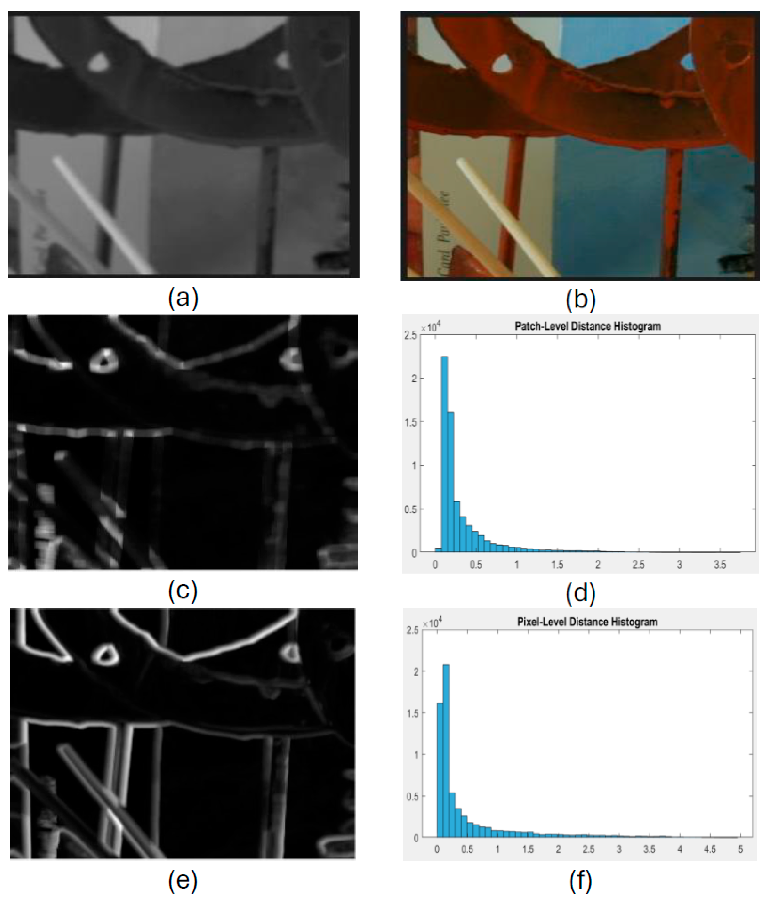
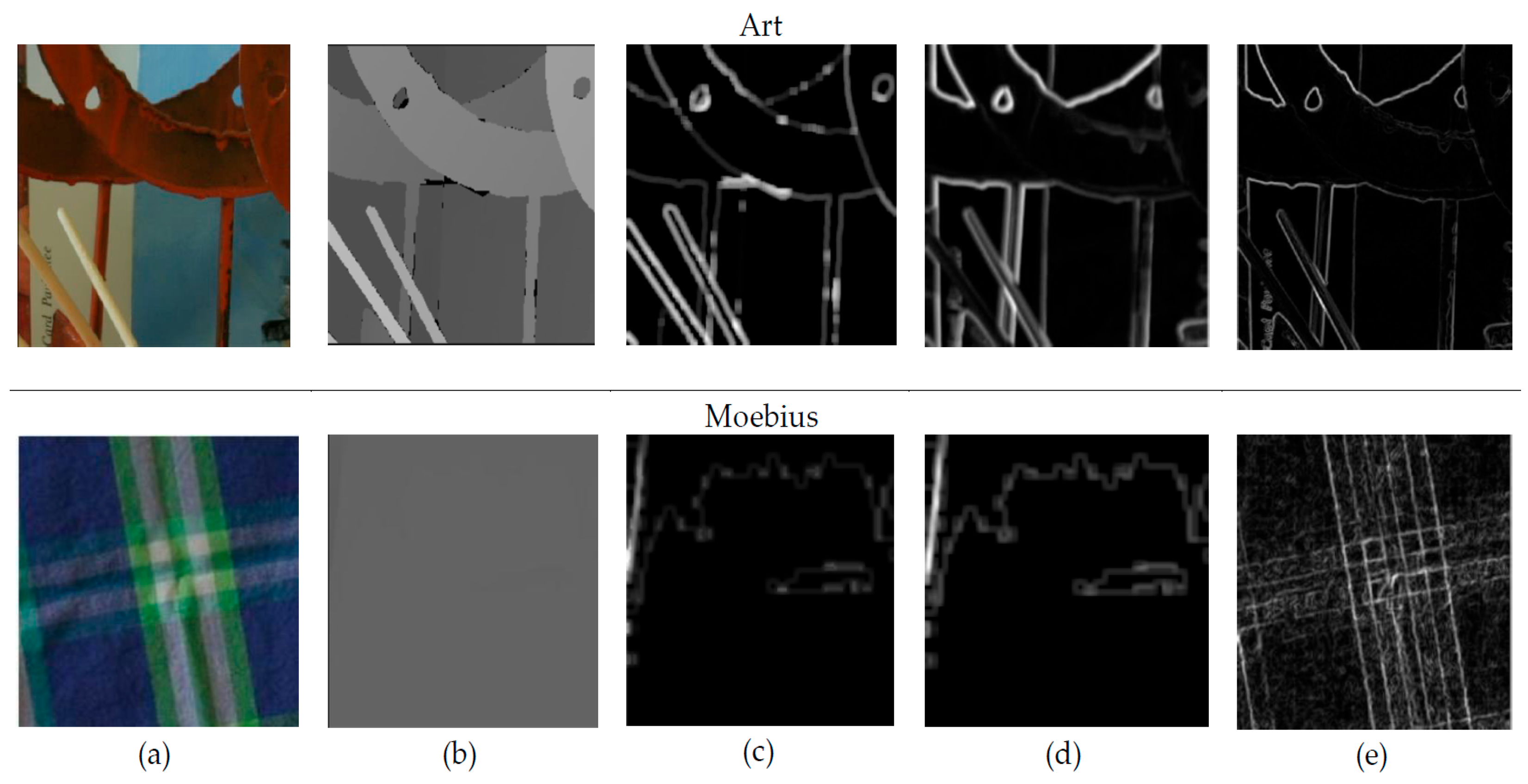
2.1. Distance Map and Adaptive Bandwidth
2.2. Local Model
2.3. Nonlocal Model
2.4. Fusion of Local and Nonlocal Outputs for Depth Upsampling
3. Experimental Results
3.1. Parameters Settings
3.2. Adaptive Bandwidth Analysis
3.3. Quantitative Results
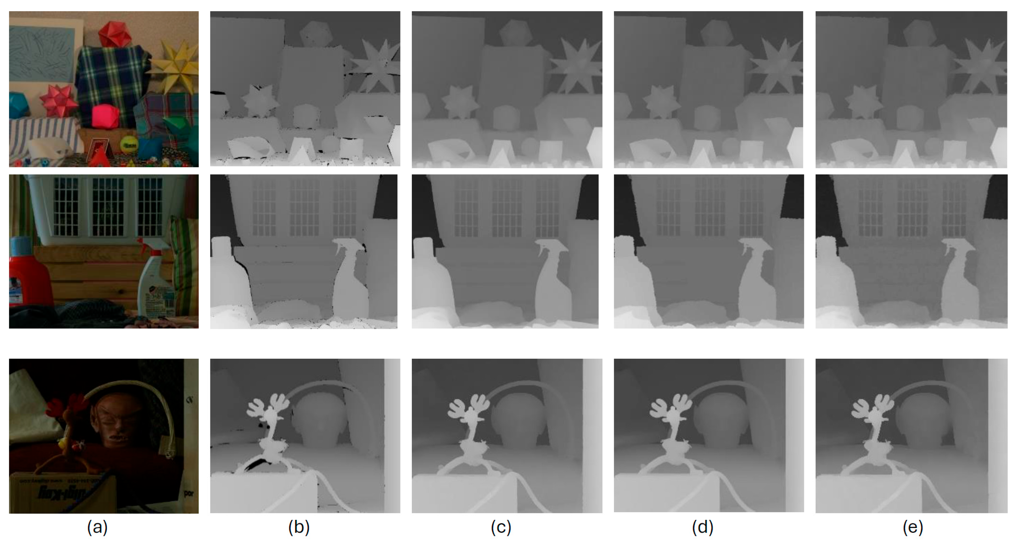
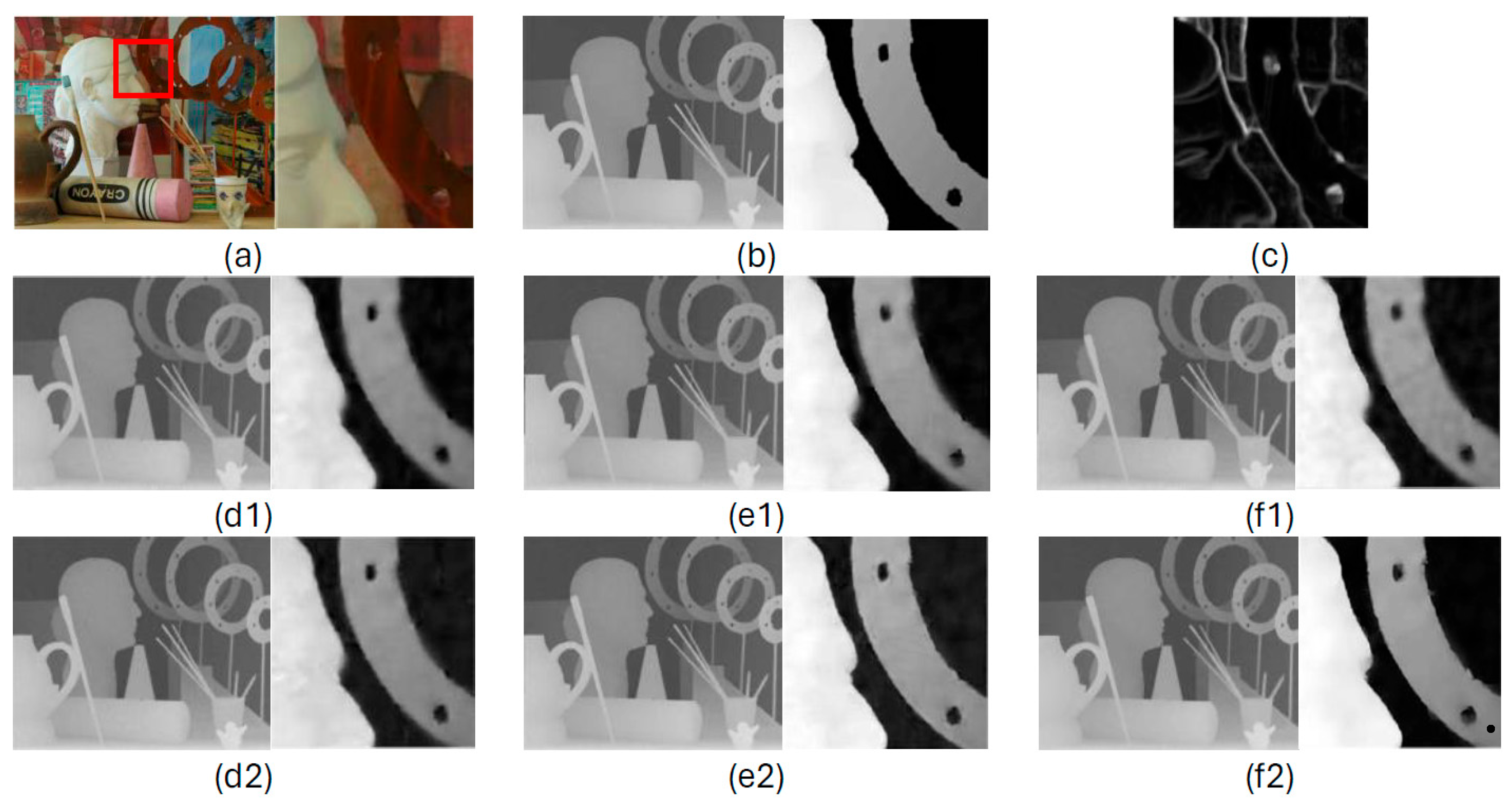
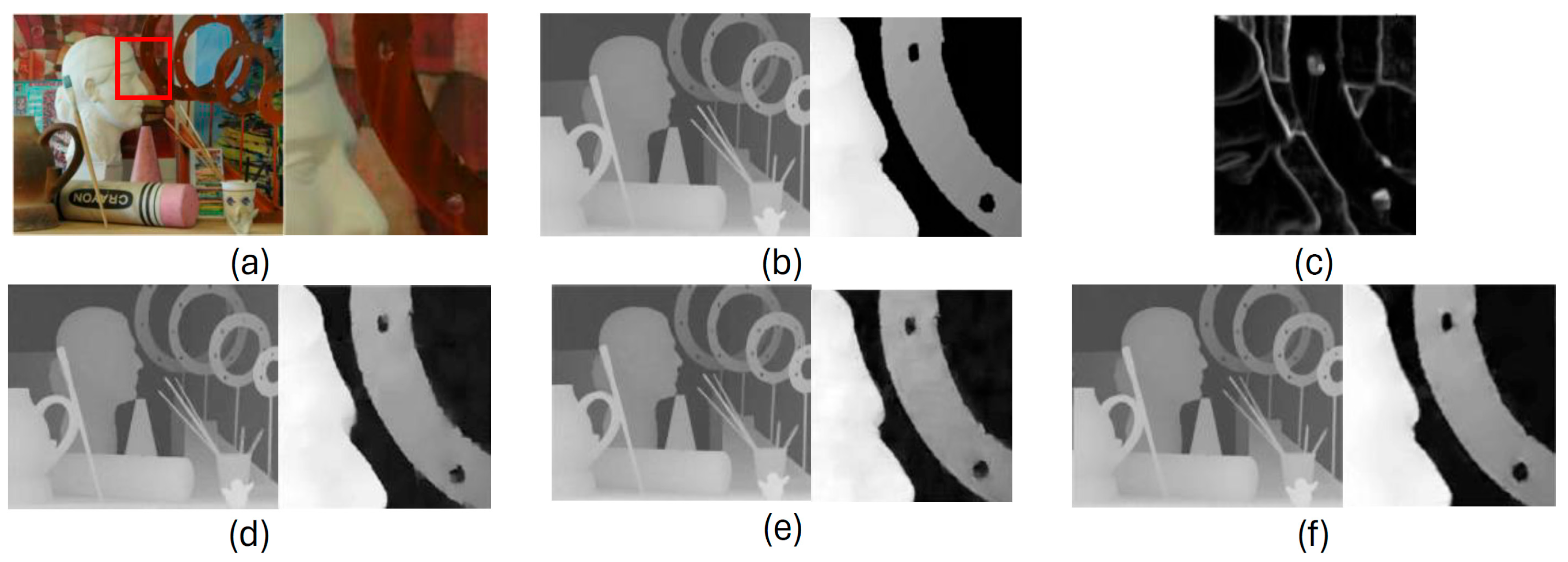
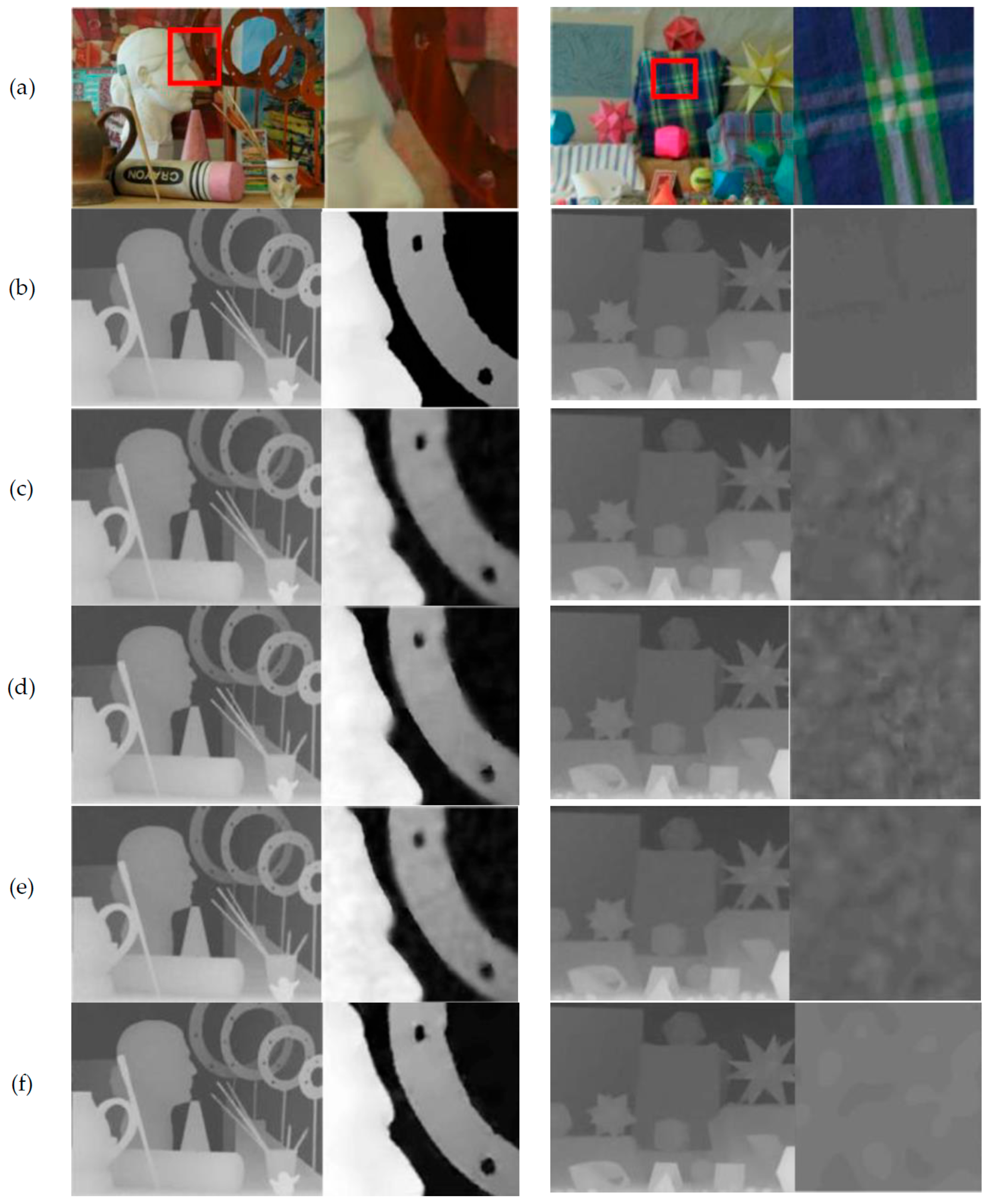
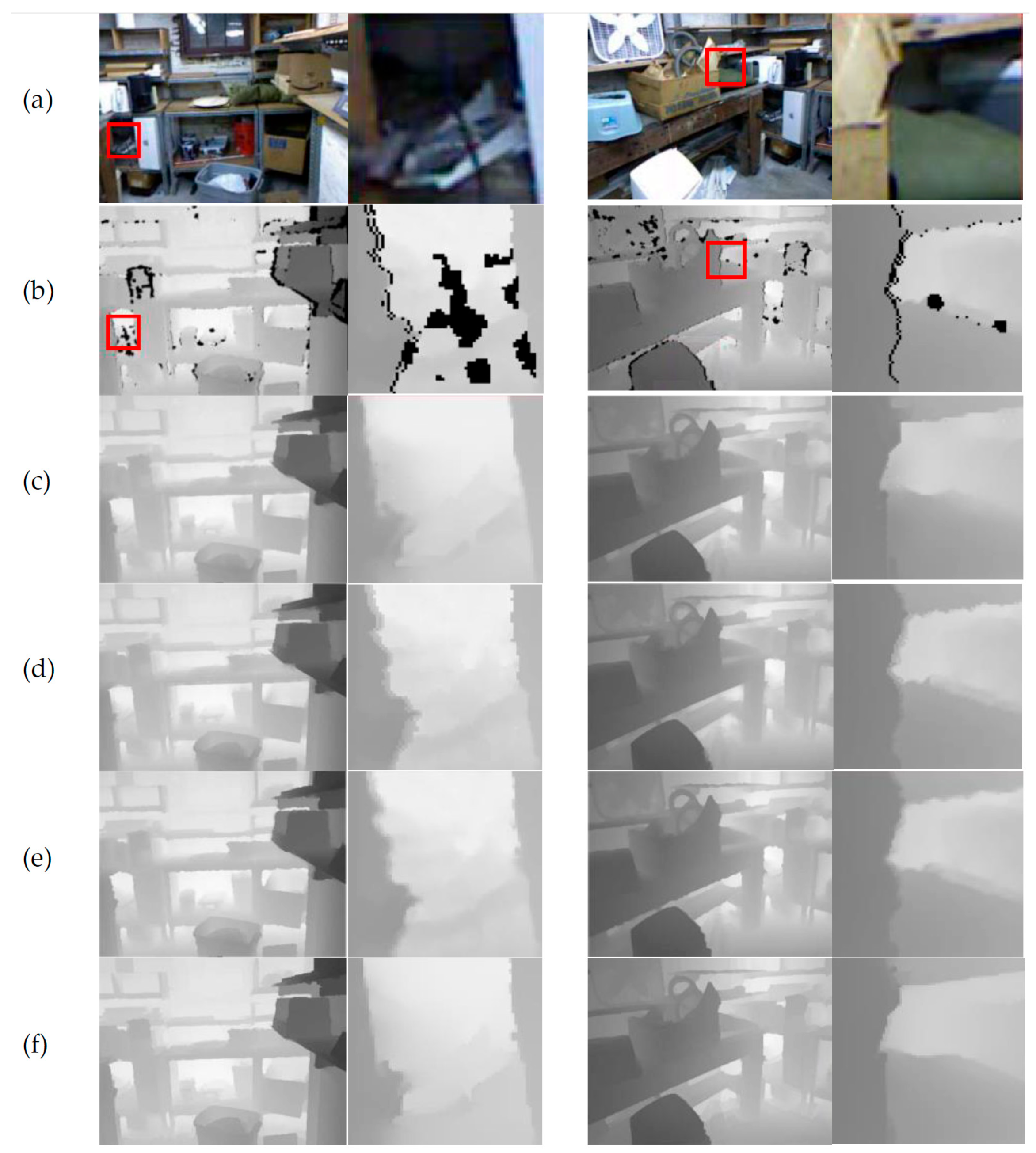
3.4. Visual Results
4. Conclusions
Author Contributions
Funding
Data Availability Statement
Conflicts of Interest
Abbreviations
| ToF | Time of Flight |
| HR | High-resolution |
| LR | Low-resolution |
| GDSR | Guided depth map super-resolution |
| SD | Static/Dynamic |
| MAE | Mean absolute error |
| RMSE | Root mean square error |
References
- Du, L.; Ye, X.; Tan, X.; Johns, E.; Chen, B.; Ding, E.; Xue, X.; Feng, J. AGO-Net: Association-Guided 3D Point Cloud Object Detection Network. IEEE Trans. Pattern Anal. Mach. Intell. 2021, 44, 8097–8109. [Google Scholar] [CrossRef] [PubMed]
- Wang, L.; Zhang, L.; Zhu, Y.; Zhang, Z.; He, T.; Li, M.; Xue, X. Progressive coordinate transforms for monocular 3d object detection. Adv. Neural Inf. Process. Syst. 2021, 34, 13364–13377. [Google Scholar]
- Han, X.F.; Laga, H.; Bennamoun, M. Image-based 3D object reconstruction: State-of-the-art and trends in the deep learning era. IEEE Trans. Pattern Anal. Mach. Intell. 2019, 43, 1578–1604. [Google Scholar] [CrossRef] [PubMed]
- Peng, S.; Jiang, C.; Liao, Y.; Niemeyer, M.; Pollefeys, M.; Geiger, A. Shape as points: A differentiable poisson solver. Adv. Neural Inf. Process. Syst. 2021, 34, 13032–13044. [Google Scholar]
- Liu, M.-Y.; Tuzel, O.; Taguchi, Y. Joint Geodesic Upsampling of Depth Images. In Proceedings of the 2013 IEEE Conference on Computer Vision and Pattern Recognition (CVPR), Portland, OR, USA, 23–28 June 2013; pp. 169–176. [Google Scholar]
- Dong, W.; Shi, G.; Li, X.; Peng, K.; Wu, J.; Guo, Z. Color-guided depth recovery via joint local structural and nonlocal low-rank regularization. IEEE Trans. Multimed. 2017, 19, 293–301. [Google Scholar] [CrossRef]
- Zhang, Y.; Ding, L.; Sharma, G. Local-linear-fitting-based matting for joint hole filling and depth upsampling of RGB-D images. J. Electron. Imaging 2019, 28, 033019. [Google Scholar] [CrossRef]
- Liu, W.; Chen, X.; Yang, J.; Wu, Q. Robust color guided depth map restoration. IEEE Trans. Image Process. 2016, 26, 315–327. [Google Scholar] [CrossRef] [PubMed]
- Zuo, Y.; Wu, Q.; Zhang, J.; An, P. Explicit edge inconsistency evaluation model for color-guided depth map enhancement. IEEE Trans. Circuits Syst. Video Technol. 2018, 28, 439–453. [Google Scholar] [CrossRef]
- Yang, M.; Cheng, Y.; Guang, Y.; Wang, J.; Zheng, N. Boundary recovery of depth map for synthesis view optimization in 3D video. In Proceedings of the IEEE International Conference on Consumer Electronics (ICCE), Las Vegas, NV, USA; 2019; pp. 1–4. [Google Scholar]
- Wang, H.; Yang, M.; Lan, X.; Zhu, C.; Zheng, N. Depth map recovery based on a unified depth boundary distortion model. IEEE Trans. Image Process. 2022, 31, 7020–7035. [Google Scholar] [CrossRef] [PubMed]
- Yang, J.; Ye, X.; Li, K.; Hou, C.; Wang, Y. Color-guided depth recovery from RGB-D data using an adaptive autoregressive model. IEEE Trans. Image Process. 2014, 23, 3443–3458. [Google Scholar] [CrossRef] [PubMed]
- Hui, T.-W.; Loy, C.C.; Tang, X. Depth map super-resolution by deep multi-scale guidance. In Proceedings of the European Conference on Computer Vision, Amsterdam, The Netherlands, 11–14 October 2016; pp. 353–369. [Google Scholar]
- Ham, B.; Cho, M.; Ponce, J. Robust image filtering using joint static and dynamic guidance. In Proceedings of the IEEE Conference on Computer Vision and Pattern Recognition (CVPR), Boston, MA, USA, 7–12 June 2015; pp. 4823–4831. [Google Scholar]
- Xie, J.; Feris, R.S.; Sun, M.-T. Edge-guided single depth image super resolution. IEEE Trans. Image Process. 2016, 25, 428–438. [Google Scholar] [CrossRef] [PubMed]
- Jiang, Z.; Hou, Y.; Yue, H.; Yang, J.; Hou, C. Depth super-resolution from RGB-D pairs with transform and spatial domain regularization. IEEE Trans. Image Process. 2018, 27, 2587–2602. [Google Scholar] [CrossRef] [PubMed]
- Diebel, J.; Thrun, S. An application of Markov random fields to range sensing. In Proceedings of the Neural Information Processing Systems, Vancouver, BC, Canada, 5–8 December 2005; pp. 291–298. [Google Scholar]
- Park, J.; Kim, H.; Tai, Y.-W.; Brown, M.S.; Kweon, I. High quality depth map upsampling for 3D-TOF cameras. In Proceedings of the IEEE International Conference on Computer Vision, Barcelona, Spain, 6–13 November 2011; pp. 1623–1630. [Google Scholar]
- Liu, W.; Chen, X.; Yang, J.; Wu, Q. Variable bandwidth weighting for texture copy artifact suppression in guided depth upsampling. IEEE Trans. Circuits Syst. Video Technol. 2017, 27, 2072–2085. [Google Scholar] [CrossRef]
- Zhong, Z.; Liu, X.; Jiang, J.; Zhao, D.; Ji, X. Guided depth map super-resolution: A survey. ACM Comput. Surv. 2023, 55, 1–36. [Google Scholar] [CrossRef]
- Hou, Y.; Zhang, H.; Yuan, X.; Su, Z.; Huang, F. NLH: A blind pixel-level non-local method for real-world image denoising. IEEE Trans. Image Process. 2020, 29, 5121–5135. [Google Scholar] [CrossRef]
- Beck, A.; Teboulle, M. A fast iterative shrinkage-thresholding algorithm for linear inverse problems. SIAM J. Imaging Sci. 2009, 2, 183–202. [Google Scholar] [CrossRef]
- Middlebury Datasets. Available online: http://vision.middlebury.edu/stereo/data/ (accessed on 8 November 2024).
- Scharstein, D.; Pal, C. Learning conditional random fields for stereo. In Proceedings of the IEEE Conference on Computer Vision and Pattern Recognition (CVPR 2007), Minneapolis, MN, USA, 17–22 June 2007. [Google Scholar]
- Hirschmüller, H.; Scharstein, D. Evaluation of cost functions for stereo matching. In Proceedings of the IEEE Conference on Computer Vision and Pattern Recognition (CVPR 2007), Minneapolis, MN, USA, 17–22 June 2007. [Google Scholar]
- Daniel, S.; Heiko, H.; York, K.; Greg, K.; Nera, N.; Xi, W.; Porter, W. High-resolution stereo datasets with subpixel accurate ground truth. In Proceedings of the German Conference on Pattern Recognition (GCPR), Münster, Germany, 2–5 September 2014; pp. 31–42. [Google Scholar]
- Silberman, N.; Hoiem, D.; Kohli, P.; Fergus, R. Indoor segmentation and support inference from RGB-D images. In Proceedings of the European Conference on Computer Vision (ECCV), Florence, Italy, 7–13 October 2012; pp. 746–760. Available online: https://cs.nyu.edu/fergus/datasets/ (accessed on 12 March 2025).
- Wilcoxon, F. Individual comparisons by ranking methods. In Breakthroughs in Statistics; Springer: New York, NY, USA, 1992; pp. 196–202. [Google Scholar]
- Montgomery, D.C.; Runger, G.C. Applied Statistics and Probability for Engineers, 6th ed.; Wiley: Hoboken, NJ, USA, 2013. [Google Scholar]
- Chen, H.; Zendehdel, N.; Leu, M.C.; Yin, Z. Fine-grained activity classification in assembly based on multi-visual modalities. J. Intell. Manuf. 2023, 35, 2215–2233. [Google Scholar] [CrossRef]

| Adaptive Bandwidth | MAE | RMSE |
|---|---|---|
| Configuration 1: Local variance | 3.15 | 4.57 |
| Configuration 2: Local variance + Patch Similarity | 1.64 | 2.44 |
| Configuration 3: Local variance + Patch Similarity + Color Gradient (Proposed Configuration) | 0.63 | 0.93 |
| AR [12] | RCG [8] | LLFM [7] | Proposed | ||||
|---|---|---|---|---|---|---|---|
| without AB | with AB | without AB | with AB | without AB | with AB | ||
| 2× sampling rate | |||||||
| Art | 1.17 | 1.03 | 0.71 | 0.65 | 0.69 | 0.59 | 0.55 (−20%) |
| Moebius | 0.95 | 0.87 | 0.55 | 0.45 | 0.57 | 0.55 | 0.43 (−21%) |
| Books | 0.98 | 0.9 | 0.57 | 0.51 | 0.54 | 0.48 | 0.42 (−22%) |
| Laundry | 1 | 0.88 | 0.54 | 0.49 | 0.61 | 0.6 | 0.41 (−24%) |
| Reindeer | 1.07 | 0.93 | 0.57 | 0.55 | 0.55 | 0.52 | 0.49 (−10%) |
| W | 0 | - | 0 | - | 0 | - | - |
| 4× sampling rate | |||||||
| Art | 1.7 | 1.58 | 1.06 | 0.97 | 0.98 | 0.89 | 0.78 (−20%) |
| Moebius | 1.2 | 1.07 | 0.76 | 0.67 | 0.75 | 0.7 | 0.63 (−16%) |
| Books | 1.22 | 1.11 | 0.78 | 0.7 | 0.71 | 0.68 | 0.58 (−18%) |
| Laundry | 1.31 | 1.15 | 0.77 | 0.69 | 0.8 | 0.73 | 0.61 (−20%) |
| Reindeer | 1.3 | 1.13 | 0.8 | 0.71 | 0.72 | 0.63 | 0.59 (−18%) |
| W | 0 | - | 0 | - | 0 | - | - |
| 8× sampling rate | |||||||
| Art | 2.93 | 2.75 | 1.72 | 1.66 | 1.68 | 1.49 | 1.37 (−18%) |
| Moebius | 1.79 | 1.58 | 1.15 | 1.08 | 1.25 | 1.18 | 0.99 (−13%) |
| Books | 1.74 | 1.64 | 2.18 | 2.11 | 2.09 | 1.97 | 1.73 (−17%) |
| Laundry | 1.97 | 1.73 | 1.12 | 1.05 | 1.15 | 1.03 | 0.96 (−14%) |
| Reindeer | 2.03 | 1.89 | 1.14 | 1.05 | 1.08 | 0.99 | 0.93 (−13%) |
| W | 0 | - | 0 | - | 0 | - | - |
| AR [12] | RCG [8] | LLFM [7] | Proposed | |||
|---|---|---|---|---|---|---|
| without AB | with AB | without AB | with AB | without AB | with AB | |
| 231.34 | 268.21 | 205.09 | 246.81 | 169.40 | 201.54 | 197.63 |
| Art | Dolls | Laundry | Moebius | Reindeer | Books | Avg | W | |
|---|---|---|---|---|---|---|---|---|
| MSG [13] | 5.84 | 2.08 | 3.89 | 2.27 | 4.62 | 2.94 | 3.61 | 0 |
| SDF [14] | 4.14 | 1.52 | 2.53 | 1.72 | 3.05 | 1.98 | 2.49 | 0 |
| LLFM [7] | 3.31 | 1.48 | 2.75 | 1.34 | 3.51 | 1.78 | 2.36 | 0 |
| RCG [8] | 3.56 | 1.42 | 2.91 | 2.05 | 3.65 | 1.65 | 2.76 | 0 |
| AR [12] | 4.07 | 1.52 | 2.70 | 1.64 | 2.86 | 2.18 | 2.5 | 0 |
| EG [15] | 4.16 | 1.53 | 2.68 | 1.56 | 3.30 | 2.15 | 2.56 | 0 |
| LN [6] | 2.62 | 1.03 | 1.66 | 1.02 | 2.14 | 1.47 | 1.66 | 0 |
| DTSR [16] | 1.57 | 0.87 | 0.98 | 0.62 | 1.19 | 1.05 | 1.04 | 2 |
| Proposed | 1.32 | 0.93 | 0.76 | 0.58 | 1.02 | 0.98 | 0.93 | - |
| Couch | Motorcycle | Pipes | Recycle | Sticks | Sword1 | Avg | W | |
|---|---|---|---|---|---|---|---|---|
| LN [6] | 3.25 | 2.77 | 4.20 | 1.40 | 1.77 | 3.10 | 2.75 | 0 |
| LLFM [7] | 3.1 | 2.63 | 4.08 | 1.15 | 1.78 | 3.06 | 2.63 | 0 |
| RCG [8] | 3.33 | 2.76 | 4.18 | 1.17 | 1.98 | 3.18 | 2.77 | 0 |
| EIEF [9] | 2.99 | 2.40 | 3.60 | 1.12 | 1.56 | 2.84 | 2.41 | 0 |
| DBR [10] | 2.71 | 2.45 | 3.54 | 1.29 | 1.30 | 2.51 | 2.3 | 0 |
| UDBD [11] | 2.51 | 2.42 | 3.59 | 0.80 | 1.90 | 2.45 | 2.28 | 2 |
| Proposed | 2.3 | 2.36 | 3.28 | 0.95 | 1.15 | 2.23 | 2.04 | - |
| Couch | Motorcycle | Pipes | Recycle | Sticks | Sword1 | Avg | W | |
|---|---|---|---|---|---|---|---|---|
| LN [6] | 9.86 | 7.13 | 9.62 | 4.47 | 3.18 | 8.40 | 7.11 | 0 |
| LLFM [7] | 11.59 | 7.45 | 10.14 | 4.6 | 3.98 | 9.33 | 7.84 | 0 |
| RCG [8] | 11.66 | 7.78 | 11.76 | 3.98 | 4.02 | 9.69 | 8.14 | 1 |
| EIEF [9] | 11.32 | 7.30 | 10.16 | 4.77 | 3.84 | 10.27 | 7.94 | 0 |
| DBR [10] | 9.68 | 7.40 | 9.39 | 4.74 | 3.06 | 8.92 | 7.2 | 0 |
| UDBD [11] | 11.22 | 7.24 | 9.43 | 3.98 | 4.71 | 8.29 | 7.5 | 1 |
| Proposed | 9.56 | 7.07 | 9.23 | 4 | 2.94 | 8.01 | 6.8 | - |
Disclaimer/Publisher’s Note: The statements, opinions and data contained in all publications are solely those of the individual author(s) and contributor(s) and not of MDPI and/or the editor(s). MDPI and/or the editor(s) disclaim responsibility for any injury to people or property resulting from any ideas, methods, instructions or products referred to in the content. |
© 2025 by the authors. Licensee MDPI, Basel, Switzerland. This article is an open access article distributed under the terms and conditions of the Creative Commons Attribution (CC BY) license (https://creativecommons.org/licenses/by/4.0/).
Share and Cite
Salehi Dastjerdi, N.; Ahmad, M.O. Depth Upsampling with Local and Nonlocal Models Using Adaptive Bandwidth. Electronics 2025, 14, 1671. https://doi.org/10.3390/electronics14081671
Salehi Dastjerdi N, Ahmad MO. Depth Upsampling with Local and Nonlocal Models Using Adaptive Bandwidth. Electronics. 2025; 14(8):1671. https://doi.org/10.3390/electronics14081671
Chicago/Turabian StyleSalehi Dastjerdi, Niloufar, and M. Omair Ahmad. 2025. "Depth Upsampling with Local and Nonlocal Models Using Adaptive Bandwidth" Electronics 14, no. 8: 1671. https://doi.org/10.3390/electronics14081671
APA StyleSalehi Dastjerdi, N., & Ahmad, M. O. (2025). Depth Upsampling with Local and Nonlocal Models Using Adaptive Bandwidth. Electronics, 14(8), 1671. https://doi.org/10.3390/electronics14081671