Research on Environmental Adaptability of Force–Position Hybrid Control for Quadruped Robots Based on Model Predictive Control

Abstract

This study proposes a force–position hybrid control method for quadruped robots based on the Model Predictive Control (MPC) algorithm, aiming to address the challenges of stability and adaptability in complex terrain environments. Traditional control methods for quadruped robots are often based on simplified models, neglecting the impact of complex terrains and unstructured environments on control performance. To enhance the real-world performance of quadruped robots, this paper employs the MPC algorithm to integrate force and position control to achieve precise force–position hybrid regulation. By transforming foot-end forces into joint torques and optimizing them using kinematic inverse solutions, the robot’s stability and motion accuracy in challenging terrains is further enhanced. In this study, a Kalman filter-based state estimation method is adopted to estimate the robot’s state in real time, enabling closed-loop control through the MPC framework, combined with kinematic inverse solutions for hybrid control. The experimental results demonstrate that the proposed MPC algorithm significantly improves the robot’s adaptability and control accuracy across various terrains. In particular, it exhibits superior performance and robustness in multi-contact and uneven terrain scenarios. This research provides a novel approach for deploying quadruped robots in dynamic and complex environments and offers strong support for further optimization of motion control strategies.

1. Introduction

1.1. Research Background

With the rapid development of robotics technology [1,2,3], quadruped robots [4,5] have demonstrated significant potential in various applications, such as disaster rescue, inspection, and military missions, owing to their superior mobility and terrain adaptability [6,7,8,9]. However, in complex terrains and dynamic environments, quadruped robots often face numerous challenges, including irregular terrain, external disturbances, and stringent real-time performance requirements. These issues significantly affect the stability and motion performance of robots, increasing uncertainty in practical missions. Therefore, improving the stability and adaptability of quadruped robots in complex environments [10,11,12] has become a key focus of research in the robotics field.

1.2. State of the Art

In the field of quadruped robotics, many researchers have proposed improved MPC [13] methods to address the challenges of complex terrains and dynamic disturbances, achieving notable progress. The ETH Zurich team [14], using the ANYmal quadruped platform, incorporated foothold constraints into MPC, enabling stable locomotion on slopes, gaps, and stepping stones through inequality constraints. The MIT Cheetah team [15] proposed a novel nonlinear predictive model (RPC) [16] that optimizes the robot’s state, foot-end positions, and ground reaction forces, significantly improving dynamic speed tracking in complex terrain. Dini Navid [17] introduced an MPC-based footstep adjustment strategy that regenerates gait patterns to maintain robot balance when subjected to sudden external disturbances. Michael Neunert [18] designed an MPC method that integrates trajectory optimization with control frameworks, improving robot performance through a unified control and estimation framework.

However, the existing studies still exhibit several limitations:

Single Control Strategy: Most studies focus solely on force control or position control, neglecting the importance of their coordination.

High Resource Consumption: Complex optimization computations increase the real-time computational burden on controllers, imposing high demands on hardware performance.

Limited Environmental Adaptability: The current methods show insufficient robustness to disturbances and adaptability to dynamic and complex environments.

1.3. Contributions of This Paper

To address the above issues, this paper proposes a force–position hybrid control method based on MPC, aiming to enhance the stability and adaptability of quadruped robots in complex terrains. The specific contributions are as follows:

Force–Position Hybrid Control: A coordinated strategy combining force control and position control is introduced, integrating force control with joint position optimization to achieve high-precision foot-end control.

State Estimation: A state estimation method based on Kalman filtering is adopted to improve real-time perception of the robot’s posture and velocity.

Kinematic Inverse Solution: By incorporating the robot’s kinematic model and attitude matrix, the foot-end position and joint angle planning are optimized to support efficient closed-loop control.

Adaptability to Complex Terrains: A control framework with high dynamic response capabilities is designed, enhancing robot stability under complex terrains and dynamic disturbances.

Through simulations and physical experiments, the proposed control method is comprehensively evaluated and verified for its adaptability and control performance in complex terrain environments. The results demonstrate that the MPC-based control framework significantly enhances the robot’s motion stability and control precision in multi-contact, uneven terrain, and dynamically disturbed scenarios. This research provides a novel approach for deploying quadruped robots in dynamic and complex environments and lays a strong foundation for the further optimization of motion control strategies.

2. Methods

2.1. Force–Position Hybrid Control Framework

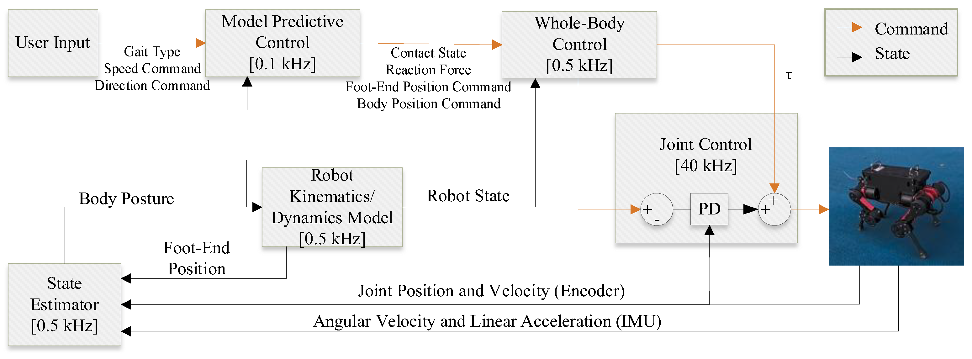
The force–position hybrid control framework aims to integrate foot-end force control and joint position control to improve the precision and robustness of robot motion. The overall framework of the force–position hybrid control system for the quadruped robot is illustrated in Figure 1.

Position Control Component: By incorporating kinematic inverse solutions, this component optimizes joint positions and foot-end poses, enabling the robot to quickly adapt to complex terrains.

Force Control Component: Using MPC, the target support forces at the robot’s foot ends are calculated to ensure stability under terrain changes or external disturbances.

Collaborative Optimization: Force and position controls are correlated through the Jacobian matrix, with the output of MPC guiding the generation of comprehensive control commands.

2.2. System Modeling

This study uses the quadruped robot Tinymal as a reference to build and simplify the structural model. The robot consists of a rigid body and four identical legs, each with three degrees of freedom (DoFs) corresponding to a lateral hip joint, a vertical hip joint, and a knee joint.

Table 1. Modified D-H parameters for the left foreleg (LF).

Joint Frame	Link Length	Height Difference	Joint Twist	Joint Angle
1	0	0	0	0
2	$L_1$	0	−π/2	${\theta }_1$
3	$L_2$	0	0	${\theta }_2$
4	$L_3$	0	0	${\theta }_3$

details the structural dimensions and joint angle constraints of the robot’s legs. Figure 2 shows both the three-dimensional design and the actual prototype of the quadruped robot, providing an overview of its mechanical structure and appearance.

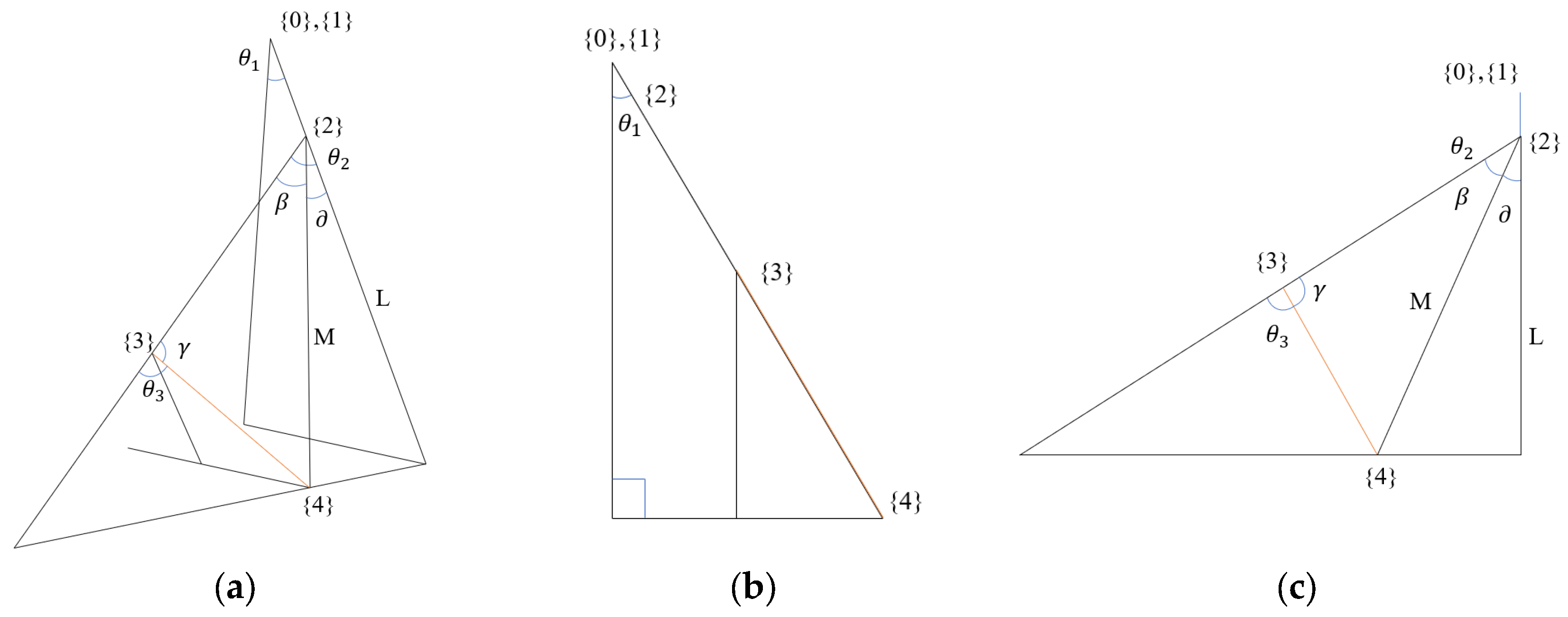
An improved Denavit–Hartenberg (D-H) parameterization method [3] is employed to define the relationships between the coordinate frames of the robot’s body and leg joints. This approach facilitates the derivation of foot-end poses under specific configurations, laying the groundwork for subsequent foot-end trajectory planning. The four legs are numbered sequentially as follows: left foreleg (LF), Left Hindleg (LH), Right Foreleg (RF), and Right Hindleg (RH). The primary coordinate systems are defined as follows:

• {W}: World coordinate frame;
• {B}: Body frame located at the robot’s center of mass;
• {0}: Base frame of the leg;
• {1}: Lateral hip joint frame;
• {2}: Vertical hip joint frame;
• {3}: Knee joint frame;
• {4}: Foot-end frame.

As all the legs share identical structural parameters, only the left foreleg (LF) is analyzed for kinematics and the establishment of the D-H coordinate system. A structural diagram illustrating the quadruped robot’s joint coordinate systems is shown in Figure 3.

The lateral hip joint angle is denoted as ${\theta }_1$, the vertical hip joint angle as ${\theta }_2$, and the knee joint angle as ${\theta }_3$. The lateral hip link length is denoted as $L_1$, the thigh link length as $L_2$, and the calf link length as $L_3$. Based on the coordinate systems established in Figure 3, the relationships among link lengths, joint angles, and height differences between joints form the modified D-H parameter table, as shown in Table 1.

By substituting the parameter values from the D-H table into the homogeneous transformation matrix equation (Equation (1)), the following transformations can be obtained:

$${}_{\begin{array}{cc}i& \end{array}}{}^{\begin{array}{l}i-1\end{array}}T=\left[\begin{array}{cccc}\cos {\theta }_i& -\sin {\theta }_i& 0& a_{i-1}\\ \sin {\theta }_i\cos {\partial }_{i-1}& \cos {\theta }_i\cos {\partial }_{i-1}& -\sin {\partial }_{i-1}& -d_i\sin {\partial }_{i-1}\\ \sin {\theta }_i\sin {\partial }_{i-1}& \cos {\theta }_i\sin {\partial }_{i-1}& \cos {\partial }_{i-1}& d_i\cos {\partial }_{i-1}\\ 0& 0& 0& 1\end{array}\right]$$

(1)

These transformations provide a clear mathematical representation of the kinematic relationships among the robot’s joint coordinate systems, forming the foundation for subsequent trajectory optimization and control strategies.

$${}_4{}^{0}T={}_1{}^{0}T{}_2{}^{1}T{}_3{}^{2}T{}_4{}^{3}T=\left[\begin{array}{cccc}{c}_{24}{c}_1& -s_{234}{c}_1& -s_1& c_1\left(L_1+L_3{c}_{23}+L_2{c}_2\right)\\ c_{234}{s}_1& -s_{244}{s}_1& c_1& s_1\left(L_1+L_3{c}_{23}+L_2{c}_2\right)\\ -s_{234}& -c_{234}& 0& -L_3{s}_{23}-L_2{s}_2\\ 0& 0& 0& 1\end{array}\right]$$

(2)

$$\begin{array}{l}{s}_i=\sin {\theta }_i, c_i=\cos {\theta }_i,\hfill \\ s_{ijk}=\sin \left({\theta }_i+{\theta }_j+{\theta }_k\right), c_{ijk}=\cos \left({\theta }_i+{\theta }_j+{\theta }_k\right), s_{ij}=\sin \left({\theta }_i+{\theta }_j\right), c_{ij}=\cos \left({\theta }_i+{\theta }_j\right)\hfill \end{array}$$

In the homogeneous transformation matrix, the first three rows and three columns represent the rotation matrix ($R$) of the foot-end relative to the leg base coordinate system, as shown in the equation. Specifically, $R$ describes the orientation of the foot-end relative to the leg base coordinate system. Meanwhile, the first three rows of the fourth column represent the position vector ($P)$ of the foot-end relative to the leg base coordinate system, as shown in the equation. Therefore, $P$ describes the position of the foot-end relative to the leg base coordinate system. Together, $P$ and $R$ define the foot-end pose relative to the leg base coordinate system through forward kinematics.

The forward kinematics of a single leg is expressed as follows:

$$\begin{array}{l}{}_4{}^{0}R=\left[\begin{array}{ccc}{c}_{24}{c}_1& -s_{23}{c}_1& -s_1\\ c_{24}{s}_1& -s_{234}{s}_1& c_1\\ -s_{234}& -c_{234}& 0\end{array}\right]\hfill \\ P=\left[\begin{array}{c}{c}_1\left(L_1+L_3{c}_{23}+L_2{c}_2\right)\\ s_1\left(L_1+L_3{c}_{23}+L_2{c}_2\right)\\ -L_3{s}_{23}-L_2{s}_2\end{array}\right]\hfill \end{array}$$

(3)

The importance of inverse kinematics analysis for quadruped robots lies in its role in determining the joint angles required to achieve a desired end-effector position (commonly referring to the foot-end position in legged robots). This is crucial for executing precise and complex tasks. Among the various methods for solving inverse kinematics, the algebraic method and geometric method are the two most commonly used. Given the relatively simple leg structure of quadruped robots, the geometric method is utilized here to solve the inverse kinematics for a single leg. Figure 4 shows the simplified diagram of a single leg.

Based on the front view of the simplified diagram of a single leg, the lateral hip joint angle can be derived using the geometric method. From Figure 4b, the relationship between the lateral hip joint angle and the foot-end position is expressed as follows:

$${\theta }_1=\arctan {\displaystyle \frac{P_y}{P_x}}$$

(4)

Similarly, based on the side view of the simplified diagram of a single leg, the geometric method can be used to derive the expressions for the hip joint angle and the knee joint angle as follows:

$${\theta }_2=\partial +\beta =\arctan {\displaystyle \frac{P_z}{\sqrt{P_x^2+P_y^2}-L_1}}+\arccos {\displaystyle \frac{L_2^2+P_z^2+{\left(\sqrt{P_x^2+P_y^2}-L_1\right)}^2-L_3^2}{2L_2\sqrt{P_x^2+{\left(\sqrt{P_x^2+P_y^2}-L_1\right)}^2}}}$$

(5)

$${\theta }_3=\pi -\gamma =\pi -\arccos {\displaystyle \frac{L_2^2+L_3^2-P_z^2-{\left(\sqrt{P_x^2+P_y^2}-L_1\right)}^2}{2L_2{L}_3}}$$

(6)

where

$$L=\sqrt{P_x^2+P_y^2}-L_1, M=\sqrt{P_z^2+{\left(\sqrt{P_x^2+P_y^2-L_1}\right)}^2}$$

$$\partial =\arctan {\displaystyle \frac{P_z}{\sqrt{P_x^2+P_y^2}-L_1}}, \beta =\arccos {\displaystyle \frac{L_2^2+P_z^2+{\left(\sqrt{P_x^2+P_y^2}-L_1\right)}^2-L_3^2}{2L_2\sqrt{P_z^2+{\left(\sqrt{P_x^2+P_y^2}-L_1\right)}^2}}}$$

(7)

$$\gamma =\arccos {\displaystyle \frac{L_2^2+L_3^2-P_z^2-{\left(\sqrt{P_x^2+P_y^2}-L_1\right)}^2}{2L_2{L}_3}}$$

2.3. State-Space Representation

A legged robot is a typical high-dimensional nonlinear system, making it difficult to establish an accurate system model. A simplified quadruped robot is illustrated in Figure 3, where $x, y, \mathrm{and} z$ represent the axes of the world coordinate system $Oxyz$ and $x_{\mathrm{b}}, y_{\mathrm{b}}, \mathrm{and} z_{\mathrm{b}}$ denote the axes of the body-fixed coordinate system $O_{\mathrm{b}}{x}_{\mathrm{b}}{y}_{\mathrm{b}}{z}_{\mathrm{b}}$. For the purpose of controller design, a typical quadruped robot as shown in Figure 3 can be represented by a simplified single rigid body model:

$$\ddot{p}={\displaystyle \frac{{\sum }_{i=1}^q{f}_i}{m}}-g$$

(8)

$${\displaystyle \frac{\mathrm{d}}{\mathrm{d}t}}\left(I\omega \right)={\sum }_{i=1}^q{r}_i\times f_i$$

(9)

$${\dot{R}}_{\mathrm{b}}^{\mathrm{w}}=\left[\omega \right]\times R_{\mathrm{b}}^{\mathrm{w}}$$

(10)

In the above equations, $p\in {ℝ}^3$ denotes the position of the robot’s center of mass in the world coordinate frame, and $f_i={\left[f_{ix},f_{iy},f_{iz}\right]}^{\mathrm{T}}\in {ℝ}^3$ represents the ground reaction force exerted by $i$-$th$ leg when in contact with the ground. The number of legs in contact is denoted by $q\in {\mathbb{N}}^{+}$. The mass of the robot is $m\in {ℝ}^{+}$. The gravitational acceleration vector is given by $g={[0,0,g]}^{\mathrm{T}}\in {ℝ}^3$. The inertia tensor of the robot expressed in the world frame is $I\in {ℝ}^3$. $\omega \in {ℝ}^3$ denotes the angular velocity of the robot (as a rigid body) expressed in the world frame. The vector from the contact point of the ground reaction force to the center of mass is denoted as $r_i\in {ℝ}^3$ and the rotation matrix from the body coordinate frame to the world coordinate frame is $R_{\mathrm{b}}^{\mathrm{w}}\in {ℝ}^{3\times 3}$. For any vectors $x,y\in {ℝ}^3$, the skew-symmetric matrix ${[x]}_{\times }\in {ℝ}^{3\times 3}$ satisfies the identity ${[x]}_{\times }y=x\times y$.

The robot’s inertia tensor $I$ in the world frame can be computed as follows:

$$I=R_{\mathrm{b}}^{\mathrm{w}}{I}_{\mathrm{b}}{\left(R_{\mathrm{b}}^{\mathrm{w}}\right)}^{\mathrm{T}}$$

(11)

where $I_{\mathrm{b}}$ is the inertia tensor in the body frame. Using Equations (10) and (11), and assuming the angular velocity $\omega$ is relatively small, the derivative of the angular momentum $I\omega$ in Equation (9) can be approximated as follows:

$${\displaystyle \frac{\mathrm{d}}{ \mathrm{d}t}}\left(I\omega \right)=I\dot{\omega }+\omega \times I\omega \approx I\dot{\omega }$$

(12)

Define the system state vector as $x=\left[p^{\mathrm{T}},{\theta }^{\mathrm{T}},v^{\mathrm{T}},{\omega }^{\mathrm{T}},g\right]$, where $v=\dot{p}$ is the linear velocity of the robot in the world frame. Then, by combining Equations (8), (9), and (12), the state-space model of the system can be expressed as follows:

$$\dot{x}=Ax+Bu,u={\left[f_1^{\mathrm{T}},\cdots ,f_q^{\mathrm{T}}\right]}^{\mathrm{T}}$$

where

$$\begin{array}{c}A=\left[\begin{array}{ccccc}{0}_{3\times 3}& 1_{3\times 3}& 0_{3\times 3}& 0_{3\times 3}& 0_{3\times 1}\\ 0_{3\times 3}& 0_{3\times 3}& R_z\left(\psi \right)& 0_{3\times 3}& 0_{3\times 1}\\ 0_{3\times 3}& 0_{3\times 3}& 0_{3\times 3}& 0_{3\times 3}& 0_{3\times 1}\\ 0_{3\times 3}& 0_{3\times 3}& 0_{3\times 3}& 0_{3\times 3}& S_{\mathrm{g}}\\ 0_{3\times 3}& 0_{3\times 3}& 0_{3\times 3}& 0_{3\times 3}& 0_{3\times 1}\\ 0_{1\times 3}& 0_{1\times 3}& 0_{1\times 3}& 0_{1\times 3}& 0\end{array}\right]\\ B=\left[\begin{array}{ccc}{0}_{3\times 3}& \cdots & 0_{3\times 3}\\ 0_{3\times 3}& \cdots & 0_{3\times 3}\\ m^{-1}{1}_{3\times 3}& \cdots & m^{-1}{1}_{3\times 3}\\ I^{-1}{\left[r_1\right]}_{\times }& \cdots & I^{-1}{\left[r_q\right]}_{\times }\\ 0_{1\times 3}& \cdots & 0_{1\times 3}\end{array}\right]\end{array}$$

(13)

Here, $S_{\mathrm{g}}={[0,0,-1]}^{\mathrm{T}}.$ For the purpose of controller implementation, the continuous-time system described by Equation (13) can be discretized using the Euler method as follows:

$$\begin{array}{c}{x}_{k+1}=A_k{x}_k+B_k{u}_k\\ A_k=1_{13\times 13}+A\mathsf{\Delta }t\\ B_k=B\mathsf{\Delta }t\end{array}$$

(14)

where $\mathsf{\Delta }t$ denotes the sampling time.

2.4. Model Predictive Control Method

MPC is an optimization-based control method that dynamically adjusts control inputs by predicting the future states of the system. The core concept of MPC involves constructing a state-space model of the system, optimizing an objective function over a receding time horizon, and generating control commands based on the current state and predicted outcomes. Using the system model, which incorporates state variables such as attitude angles, positions, and control inputs, the MPC controller predicts the optimal foot-end forces required for stable operation.

By discretizing the simplified dynamics model, the problem is transformed into a quadratic programming (QP) optimization problem. The predicted optimal foot-end forces are then used as feedforward inputs to enable the robot to achieve stable and rapid motion. The discrete finite-horizon predictive controller calculates the desired foot-end contact forces for quadruped robots.

In a typical MPC process, at each iteration, the controller starts from the current state and determines the optimal sequence of control inputs and corresponding state trajectories over a finite prediction horizon, considering constraints on both control inputs and state trajectories. This process is repeated at every time step, requiring only the initial computation of the control input trajectory’s time step.

The standard formulation of the MPC problem is as follows:

$$\begin{array}{l}\underset{x,u}{\min }{\displaystyle {\displaystyle \sum }_{k=0}^{n-1}}{\parallel x_{k+1}-x_{k+1}^{\mathrm{r}}\parallel }_{{\varrho }_k}+{\parallel u_k\parallel }_{R_k}\hfill \\ \mathrm{s}. \mathrm{t}. x_{k+1}=A_k{x}_k+B_k{u}_k,k=0,\cdots ,n-1,\hfill \\ \left|f_{ix}\right|⩽\mu \left|f_{iz}\right|,\left|f_{iy}\right|⩽\mu \left|f_{iz}\right|,0⩽f_{iz}⩽f_{iz,\max }\hfill \end{array}$$

(15)

In the above equations, $x_{k+1}^{\mathrm{r}}\in {ℝ}^{13}$ denotes the reference signal. $Q_k\in {ℝ}^{13\times 13},R_k\in {ℝ}^{3q\times 3q}$ are positive definite diagonal matrices representing the weight matrices for tracking error and control input, respectively. $\mu \in {ℝ}^{+}$ denotes the coefficient of friction between the foot and the ground.

To facilitate the solution of the MPC problem, the $n$-step optimization can be further transformed into a quadratic programming (QP) problem. Based on Equation (14), we obtain the following formulation:

$$X=A_{\mathrm{qp}}{x}_0+B_{\mathrm{qp}}U$$

(16)

In the above equations, $X={\left[x_1^{\mathrm{T}},\cdots ,x_n^{\mathrm{T}}\right]}^{\mathrm{T}}\in {ℝ}^{13n}$ represents all the system states over the prediction horizon $n$ and $U={\left[u_0^{\mathrm{T}},\cdots ,u_{n-1}^{\mathrm{T}}\right]}^{\mathrm{T}}\in {ℝ}^{12n}$ represents all the control inputs over the same horizon. The matrices $A_{\mathrm{qp}}\in {ℝ}^{13n\times 13}$ and $B_{\mathrm{qp}}\in {ℝ}^{13n\times 3qn}$ are defined as follows:

$$\begin{gathered} A_{\mathrm{qP}}=\left[\begin{array}{c}{A}_0\\ A_1{A}_0\\ ⋮\\ A_{n-1}\cdots A_0\end{array}\right] \\ {B}_{\mathrm{qP}}=\left[\begin{array}{cccc}{B}_0& 0_{13\times 3q}& 0& 0_{13\times 3q}\\ A_1{B}_0& B_1& 0& 0_{13\times 3q}\\ ⋮& ⋮& \ddots & 0\\ A_{n-1}\cdots A_1{B}_0& A_{n-1}\cdots A_2{B}_0& \cdots & B_{n-1}\end{array}\right] \end{gathered}$$

(17)

Using Equation (16), the optimization objective function for the QP problem can be constructed as follows:

$$\underset{U}{\min }{\parallel A_{\mathrm{qp}}{x}_0+B_{\mathrm{qp}}U-X_{\mathrm{ref}}\parallel }_{{\varrho }_{\mathrm{qP}}}+{\parallel U\parallel }_{R_{\mathrm{qp}}}$$

(18)

In the above equations, $X_{\mathrm{ref} }={\left[{\left(x_1^{\mathrm{r}}\right)}^{\mathrm{T}},\cdots ,{\left(x_k^{\mathrm{r}}\right)}^{\mathrm{T}}\right]}^{\mathrm{T}}\in {ℝ}^{13n}$ denotes the reference signals over the prediction horizon. The positive definite diagonal matrices $Q_{\mathrm{qp}}\in {ℝ}^{13n\times 13n} \mathrm{and} R_{\mathrm{qp}}\in {ℝ}^{3qn\times 3qn}$ represent the weight matrices for tracking error and control inputs, respectively. These are constructed by assembling the individual diagonal matrices $Q_k$ and $R_k$ for each time step $k$ within the horizon.

By rearranging Equation (18) and considering the friction constraints, the final QP problem can be formulated as follows:

$$\begin{array}{r}\underset{U}{\min }{\displaystyle \frac{1}{2}}{U}^{\mathrm{T}}HU+U^{\mathrm{T}}F\\ \mathrm{s}. \mathrm{t}. CU⩽\overline{c}\end{array}$$

(19)

where

$$\begin{gathered} \begin{array}{c}H=2\left(B_{\mathrm{qp}}^{\mathrm{T}}{Q}_{\mathrm{qp}}{B}_{\mathrm{qp}}+R_{\mathrm{qp}}\right)\\ F=2B_{\mathrm{qp}}^{\mathrm{T}}{Q}_{\mathrm{qp}}\left(A_{\mathrm{qp}}{x}_0-X_{\mathrm{ref}}\right)\\ C=\left[\begin{array}{cccc}{S}_U& 0_{6\times 3}& \cdots & 0_{6\times 3}\\ 0_{6\times 3}& S_U& \cdots & 0_{6\times 3}\\ 0_{6\times 3}& 0_{6\times 3}& \ddots & \cdots \\ 0_{6\times 3}& 0_{6\times 3}& \cdots & S_U\end{array}\right]\\ S_U=\left[\begin{array}{ccc}-1& 0& -\mu \\ 0& -1& -\mu \\ 1& 0& -\mu \\ 0& 1& -\mu \\ 0& 0& 1\\ 0& 0& -1\end{array}\right]\end{array} \\ \begin{array}{c}\overline{c}={\left[\begin{array}{llll}{c}_0\hfill & c_0\hfill & \cdots \hfill & c_0\hfill \end{array}\right]}^{\mathrm{T}}\\ c_0=\left[\begin{array}{llllll}0\hfill & 0\hfill & 0\hfill & 0\hfill & {\overline{f}}_z\hfill & 0\hfill \end{array}\right]\end{array} \end{gathered}$$

(20)

${\overline{f}}_z\in {ℝ}^{+}$ is a given constant, representing the maximum allowable pressure in the $z$-axis direction. By solving the standard QP problem given in Equation (19), the control inputs $U$ for all the time steps within the prediction horizon can be obtained. At the current time step, the input $u_0$ from the most recent time step can be extracted as the system input $u_{\mathrm{mpc}}$ to control the quadruped robot.

2.5. State Estimation Using Kalman Filter

The Kalman filter is a widely used method for the real-time estimation of a robot’s state, including its position, velocity, and orientation. It operates through a predict–update mechanism, which combines predictions of the state and covariance with real-time measurements to enhance estimation accuracy. During the prediction stage, the filter estimates the state and updates the covariance based on a system model and process noise. In the update stage, the filter corrects the predicted state using the measured values, adjusting the state estimate based on the Kalman gain. This method provides precise state estimates that are essential for real-time control and are used as inputs for the MPC algorithm.

3. Simulation Experiment

To validate the effectiveness of the proposed control algorithm, a comprehensive simulation framework for quadruped robot motion control was developed using MATLAB R2024a. The simulation was conducted for a total duration of 3 s, with a time step of 0.01 s, resulting in a simulation frequency of 100 Hz. The robot’s structural parameters were initialized, including a body length of 0.2898 m, width of 0.124 m, height of 0.200 m, and a total weight of 8 kg. The leg parameters, such as hip length (0.070 m), thigh length (0.160 m), and shin length (0.190 m), were defined, and the robot’s total inertia was calculated based on these dimensions, considering gravitational acceleration (9.81 m/s²). The initial position and orientation of the robot were set to [0.000, 0.000, 0.200] m and [0, 0, 0] radians, respectively, while the desired target position and orientation were set to [0.500, 0.500, 0.200] m and [0, 0, π/7] radians. Motion parameters, including the expected linear velocity of [0.300, 0.000, 0.000] m/s and angular velocity of [0.000, 0.000, 0.000] rad/s, were also initialized. For gait generation, the cycle duration was set to 0.5 s, with a load factor of 0.5. This step corresponds to one complete cycle of robot movement, which includes the support and swing phases. Foot trajectories were generated using B-spline curves to ensure smooth movement. Predefined foot-end forces were set based on the robot’s weight, with a friction coefficient of 0.3 between the feet and the ground, accounting for both the support and swing phases.

To control the robot’s motion, an MPC algorithm was employed with a prediction horizon of 30 steps and a prediction time of 0.02 s. The simulation time step was set to 0.01 s, and weight matrices for position, velocity, and foot-end forces were defined to minimize errors and control efforts. These initialization steps provided a solid foundation for the simulation, ensuring the accurate simulation of the robot’s motion control and enabling the effective validation of the proposed control algorithm. The control inputs, such as joint angles, velocities, and foot-end forces, were computed by the MPC algorithm, which continuously adjusted the robot’s movements to achieve the desired trajectory.

3.1. Path Planning and State Generation

A desired motion path was generated using a path generation function, with the initial target state aligned with the robot’s starting state. Throughout the simulation, the target states and current states were iteratively updated to ensure smooth movement along the planned trajectory.

3.2. Model Predictive Control

The proposed MPC framework was employed to compute the optimal control inputs. A Hessian matrix and quadratic programming (QP) constraints were constructed based on the robot’s dynamic model, foot-end states, and physical constraints. An optimizer then solved the QP problem to generate control inputs, which were subsequently used to update the robot’s states according to the system’s state equation.

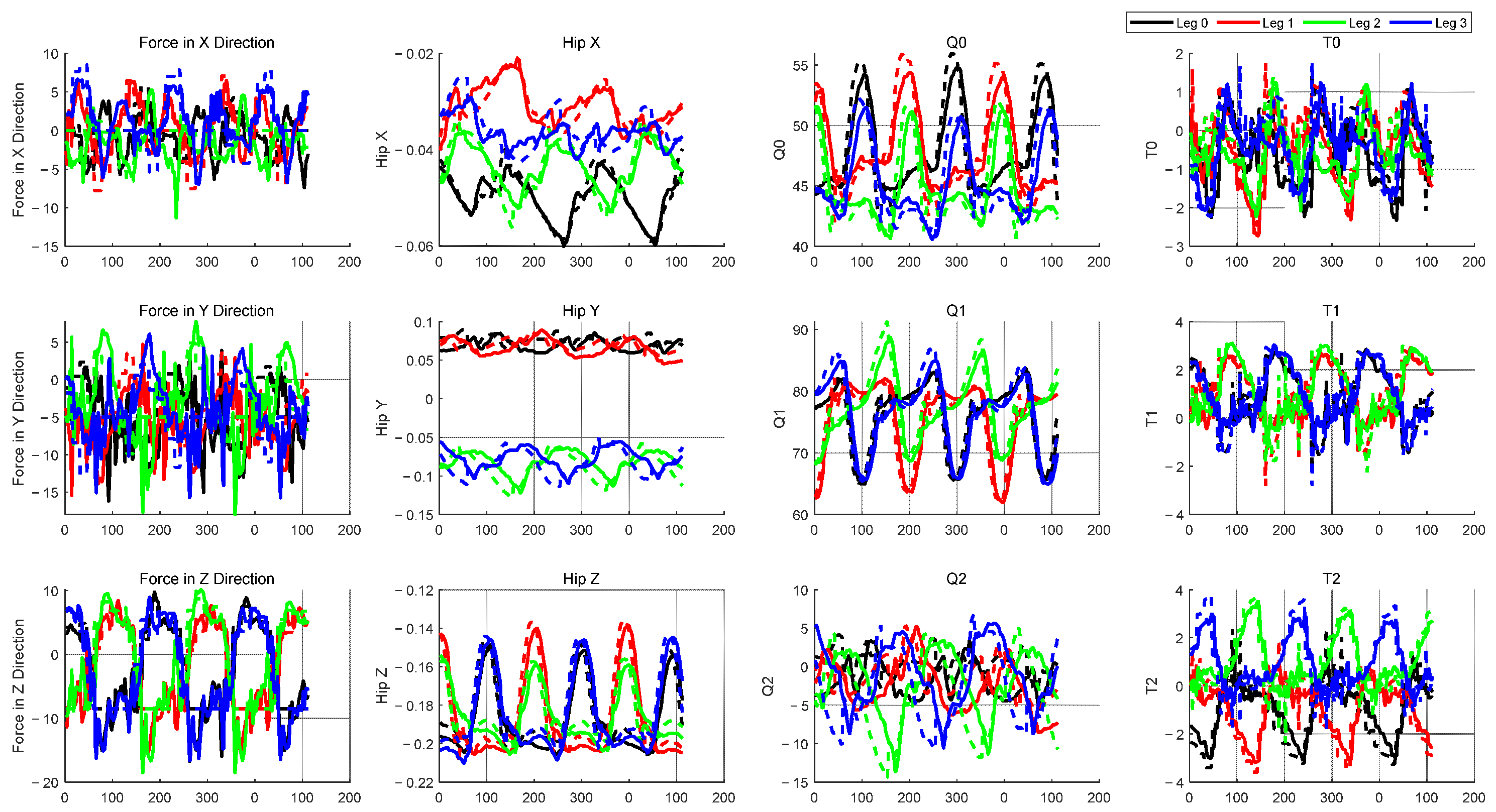
3.3. Motion Simulation and Visualization

The simulation dynamically visualized the robot’s motion and provided insights into various aspects of its performance:

• Walking trajectory: The path of the robot’s center of mass and foot-end positions over time.
• Foot-end forces: Visualization of the ground reaction forces exerted by each leg during the gait cycle.
• Joint torques from QP optimization: Analysis of the computed joint torques for the legs, highlighting the efficiency of the QP-based control strategy.
• Joint parameter outputs: Detailed charts showing joint angles, velocities, and accelerations over time.

These results are illustrated in Figure 5 (walking trajectory of the robot), Figure 6 (foot-end forces and joint torques derived from QP optimization), and Figure 7 (joint parameters, including angles and velocities).

3.4. Conclusion of Simulation Results

The simulation results demonstrate that the proposed control algorithm effectively enables stable quadruped robot motion in a simulated environment. The robot successfully tracks the desired trajectory, dynamically adjusts its posture during different gait phases, and ensures smooth transitions between the support and swing phases. The visualizations and output data provide robust theoretical and practical insights, paving the way for future real-world validations and physical experiments.

4. Physical Experiments

To validate the proposed control algorithm beyond simulations, a series of physical experiments were conducted on a quadruped robot. These experiments aimed to evaluate the robot’s stability, adaptability, and computational efficiency across diverse real-world environments and scenarios.

4.1. Experimental Setup

4.1.1. Hardware Configuration

The physical quadruped robot is equipped with the following:

Sensors: Inertial measurement units (IMUs) for posture estimation, joint encoders for joint state monitoring, and foot-end force sensors for ground reaction feedback.

Actuators: High-precision servo motors enabling smooth and precise joint control.

Controller: A real-time onboard control unit with sufficient computational resources to run the proposed MPC algorithm at 100 Hz.

4.1.2. Control Modes

The experiments were conducted in two modes to comprehensively evaluate the control algorithm:

Manual Control Mode: The robot was operated using a remote controller, allowing the operator to manually adjust its speed, direction, and gait transitions. This mode focused on testing the robot’s responsiveness and adaptability.

Path Planning Mode: The robot followed a predefined trajectory, generated by the path planning module, to evaluate its ability to autonomously track a desired path while maintaining stability and efficiency.

4.1.3. Testing Environments

The quadruped robot was tested in various environments, as depicted in Figure 8, including a runway, grassland, football field, and laboratory.

• Runway: A flat and stable surface representing ideal conditions for basic locomotion and trajectory tracking.
• Grassland: An uneven, soft terrain for testing adaptability to external disturbances such as slipping or sinking.
• Football Field: An artificial turf field requiring stability during rapid turning and dynamic speed changes.
• Laboratory: A controlled environment for precise maneuvers, such as narrow-path walking and obstacle crossing.

Figure 8. Testing environments: (a) runway, (b) grassland, (c) football field, and (d) laboratory.

Figure 8. Testing environments: (a) runway, (b) grassland, (c) football field, and (d) laboratory.

4.2. Experimental Procedure

The experiments were conducted in the following steps:

Setup: The robot was initialized with either manual control commands or a predefined path planning trajectory, depending on the mode.

Task Execution: The robot performed tasks such as straight-line walking, turning, variable-speed motion, and obstacle crossing in each environment.

Disturbance Testing: In the grassland and football field scenarios, random external pushes or terrain irregularities were introduced to evaluate recovery performance.

Data Collection: Sensor data, including joint angles, foot-end positions, ground reaction forces, and energy consumption, were recorded for offline analysis.

Figure 9 presents the posture data of the robot recorded during locomotion, illustrating its stability and motion characteristics. The ground reaction forces (GRFs) on all four legs during motion are shown in Figure 10, reflecting the dynamic load distribution and interaction with the terrain.

4.3. Results and Analysis

The performance metrics for both the manual control and path planning modes are summarized in

Table 2. Performance metrics of the quadruped robot under different terrain conditions in manual control and path planning modes.

Metric Category	Specific Metric	Definition	Runway	Grassland	Football Field	Laboratory
Stability	Trajectory Error (MSE)	Mean squared error between actual and desired trajectories (cm2).	<2 cm2	<5 cm2	<5 cm2	<3 cm2
	Posture Deviation	Standard deviation of roll and pitch angles (°).	±1°	±1°	±1°	±1°
	Foot-End Force Variation	Standard deviation of foot contact forces (N).	<3 N	<7 N	<6 N	<4 N
Adaptability	Disturbance Recovery Time	Time to regain stability after external disturbances (ms).	<400 ms	<500 ms	<450 ms	<300 ms

, covering key indicators of stability and adaptability across different terrains.

5. Conclusions

This study presents a force–position hybrid control method for quadruped robots based on the MPC algorithm, addressing the challenges of stability and adaptability in complex terrain environments. Unlike traditional control methods that rely on simplified models and often overlook the influence of unstructured terrains, the proposed approach integrates force and position control to achieve the precise regulation of foot-end forces and joint positions. By transforming foot-end forces into joint torques and optimizing them through kinematic inverse solutions, the algorithm significantly enhances the robot’s stability and motion accuracy in challenging environments.

The Kalman filter-based state estimation method further supports the control framework by providing real-time state information, enabling closed-loop control through the MPC framework. This ensures dynamic adaptability and precise regulation of the robot’s movements, even in scenarios with multi-contact and uneven terrains.

5.1. Key Findings

5.1.1. Improved Stability and Adaptability

The experimental results demonstrate that the proposed MPC algorithm effectively maintains the robot’s posture stability and balanced force distribution across all the tested terrains. Even in dynamic and unstructured environments, the robot exhibits low trajectory errors, minimal posture deviations, and rapid recovery from external disturbances.

5.1.2. Robust Performance Across Diverse Terrains

On flat surfaces, the robot achieves high trajectory tracking accuracy with minimal control errors.

On uneven terrains such as grassland and artificial turf, the hybrid control method enables rapid gait adjustments and stable locomotion, with recovery times under 500 ms from external disturbances.

5.1.3. Real-Time Control and Energy Efficiency

The integration of kinematic inverse solutions reduces computational complexity, enabling real-time control at a frequency of 100 Hz. Energy consumption measurements further confirm the efficiency of the proposed control strategy, with average power usage well optimized across all the scenarios.

5.2. Significance and Future Work

The proposed force–position hybrid control approach provides a novel solution for deploying quadruped robots in dynamic and complex environments. It demonstrates superior adaptability and robustness in real-world applications, offering strong support for further optimization of motion control strategies. Future work will focus on the following:

• Expanding the framework to handle dynamic obstacle avoidance and cooperative multi-robot systems.
• Enhancing computational efficiency to scale the algorithm for higher degrees of freedom and more complex terrains.
• Exploring learning-based methods to further improve adaptability in highly unpredictable environments.

By addressing these directions, the proposed control framework aims to contribute to the advancement of robust and intelligent quadruped robotic systems for practical deployment in diverse real-world applications.

References

- Biswal, P.; Mohanty, P.K. Development of quadruped walking robots: A review. Ain Shams Eng. J. 2021, 12, 2017–2031. [Google Scholar] [CrossRef]
- Fukuhara, A.; Gunji, M.; Masuda, Y. Comparative anatomy of quadruped robots and animals: A review. Adv. Robot. 2022, 36, 612–630. [Google Scholar] [CrossRef]
- Fan, Y.; Pei, Z.; Wang, C.; Li, M.; Tang, Z.; Liu, Q. A Review of Quadruped Robots: Structure, Control, and Autonomous Motion. Adv. Intell. Syst. 2024, 6, 2300783. [Google Scholar] [CrossRef]
- Zhu, X.; Wang, M.; Ruan, X.; Chen, L.; Ji, T.; Liu, X. Adaptive Motion Skill Learning of Quadruped Robot on Slopes Based on Augmented Random Search Algorithm. Electronics 2022, 11, 842. [Google Scholar] [CrossRef]
- Kumar, A.; Fu, Z.; Pathak, D.; Malik, J. Rma: Rapid motor adaptation for legged robots. arXiv 2021, arXiv:2107.04034. [Google Scholar]
- Kim, J.; Kang, T.; Song, D.; Yi, S.-J. Design and Control of a Open-Source, Low Cost, 3D Printed Dynamic Quadruped Robot. Appl. Sci. 2021, 11, 3762. [Google Scholar] [CrossRef]
- Di Carlo, J.; Wensing, P.M.; Katz, B.; Bledt, G.; Kim, S. Dynamic locomotion in the mit cheetah 3 through convex model-predictive control. In Proceedings of the 2018 IEEE/RSJ International Conference on Intelligent Robots and Systems (IROS), Madrid, Spain, 1–5 October 2018; IEEE: New York, NY, USA, 2018; pp. 1–9. [Google Scholar]
- Minniti, M.V.; Grandia, R.; Farshidian, F.; Hutter, M. Adaptive CLF-MPC with application to quadrupedal robots. IEEE Robot. Autom. Lett. 2021, 7, 565–572. [Google Scholar] [CrossRef]
- Lee, J.; Hwangbo, J.; Wellhausen, L.; Koltun, V.; Hutter, M. Learning quadrupedal locomotion over challenging terrain. Sci. Robot. 2020, 5, eabc5986. [Google Scholar] [CrossRef] [PubMed]
- Zhou, K.; Li, C.; Li, C.; Zhu, Q. Motion planning method for quadruped robots walking on unknown rough terrain. J. Mech. Eng. 2020, 56, 210–219. [Google Scholar]
- Xu, R.; Zhao, C.; Li, J.; Hu, J.; Hou, X. A Hybrid Improved-Whale-Optimization–Simulated-Annealing Algorithm for Trajectory Planning of Quadruped Robots. Electronics 2023, 12, 1564. [Google Scholar] [CrossRef]
- Chen, Z.; Zhan, G.; Jiang, Z.; Zhang, W.; Rao, Z.; Wang, H.; Li, J. Adaptive impedance control for docking robot via Stewart parallel mechanism. ISA Trans. 2024, 155, 361–372. [Google Scholar] [CrossRef] [PubMed]
- Kim, D.; Di Carlo, J.; Katz, B.; Bledt, G.; Kim, S. Highly dynamic quadruped locomotion via whole-body impulse control and model predictive control. arXiv 2019, arXiv:1909.06586. [Google Scholar]
- Grandia, R. Perceptive and Dynamic Locomotion Through Nonlinear Model Predictive Control. Ph.D. Thesis, ETH Zurich, Zürich, Switzerland, 2022. [Google Scholar]
- Bledt, G.; Powell, M.J.; Katz, B.; Di Carlo, J.; Wensing, P.M.; Kim, S. MIT Cheetah 3: Design and Control of a Robust, Dynamic Quadruped Robot. In Proceedings of the 2018 IEEE/RSJ International Conference on Intelligent Robots and Systems (IROS), Madrid, Spain, 1–5 October 2018; pp. 2245–2252. [Google Scholar]
- Ding, Y.; Pandala, A.; Li, C.; Shin, Y.-H.; Park, H.-W. Representation-Free Model Predictive Control for Dynamic Motions in Quadrupeds. IEEE Trans. Robot. 2021, 37, 1154–1171. [Google Scholar] [CrossRef]
- Dini, N.; Majd, V.J. An MPC-based two-dimensional push recovery of a quadruped robot in trotting gait using its reduced virtual model. Mech. Mach. Theory 2020, 146, 103737. [Google Scholar] [CrossRef]
- Neunert, M.; De Crousaz, C.; Furrer, F.; Kamel, M.; Farshidian, F.; Siegwart, R.; Buchli, J. Fast nonlinear model predictive control for unified trajectory optimization and tracking. In Proceedings of the 2016 IEEE International Conference on Robotics and Automation (ICRA), Stockholm, Sweden, 16–21 May 2016; IEEE: New York, NY, USA, 2016; pp. 1398–1404. [Google Scholar]