Multi-Objective Day-Ahead Scheduling for Air Conditioning Load Considering Dynamic Carbon Emission Factor

Abstract

The traditional optimal scheduling of air conditioning load has traditionally focused on improving user comfort and reducing electricity costs. However, research on carbon emissions generated during the operation of air conditioning is still in the developmental stage. Currently used average carbon emission factors in carbon-emission studies face challenges such as delayed data updates and difficulty in reflecting spatiotemporal variations. These issues contribute to the inaccurate quantification of carbon emissions, creating a challenging situation, which does not meet the development needs of green power systems under the “dual carbon goals”. Therefore, this paper proposes a multi-objective scheduling method for cooling-dominant air conditioning load considering the dynamic carbon emission factor (CEF), in conjunction with real-time spatiotemporal data from the electricity grid model, generates the electric carbon factor for each moment throughout the day. Firstly, while considering user comfort, the dynamic CEF-based carbon-emission cost and electricity cost are fused into the user’s comprehensive electricity cost, and a multi-objective optimization model for day-ahead scheduling of air conditioning loads is established. In addition, the above model is solved by the NSGA-II algorithm to obtain the Pareto front composed of non-dominated solutions. Then, the best compromise solution is objectively selected through gray target decision (GTD) to provide scientific decision-making for day-ahead scheduling of cooling-dominant air conditioning loads. Finally, four users with different air conditioning loads and room temperature requirements are designed to verify the effectiveness of the proposed strategy. The simulation results illustrate that compared with single-objective optimization and simple multi-objective decision-making methods, the proposed strategy possesses a stronger trade-off ability, which can greatly reduce the comprehensive electricity cost while ensuring user comfort.

1. Introduction

The greenhouse effect has led to increasingly severe global warming. To address this issue, countries worldwide have adopted various energy-saving and carbon-reduction measures. Overall, these measures aim to set net-zero emissions targets [1], guiding low-carbon development across industries through the implementation of carbon tax policies [2,3], rational carbon-pricing mechanisms, and the establishment of carbon trading markets. Currently, over 130 countries and regions globally have proposed net-zero emissions or carbon neutrality targets.

As the leading industry in China’s coal-consumption and carbon-intensive operations, the power sector is instrumental in attaining emission-reduction goals by integrating advanced energy-saving technologies and transitioning to sustainable resource management. As participants, consumers are empowered to modify their power-usage patterns for optimizing associated economic and environmental gains. To date, numerous theoretical studies and engineering practices have been conducted on user-side optimized scheduling in electricity carbon markets [4]. Reference [5] designed a Nash bargaining method to obtain Pareto optimal solutions for data center operators and users under emergency demand-response scenarios, effectively reducing additional carbon emissions caused by improper data center scheduling. Additionally, reference [6] proposed a carbon-pricing method for electricity consumers that incorporates carbon costs into electricity prices to reduce emissions, demonstrating that carbon price signals possess similar influence capabilities as electricity price signals. Reference [7] developed a demand-response approach called smart grid resource allocation, which quantifies carbon taxes while integrating carbon emissions with electricity pricing. Reference [8] compared the carbon-reduction performance between marginal emission factor-based load-shifting and price-based load-shifting methods, with simulation results demonstrating that the former approach exhibited superior carbon-reduction performance. Reference [9] established a novel low-carbon optimal scheduling method based on demand-responsive carbon intensity control, achieving both emission reduction and improved economic benefits for electricity consumers.

While existing research primarily focuses on optimizing coordination between generation and demand sides, it neglects the impact of carbon-emission factors in electricity supply–demand scheduling. Furthermore, reference [10] investigated carbon-emission factors, utilizing average CEF methodology for calculating indirect greenhouse gas outputs from power consumption. Although this method offers simplicity and ease of implementation in emission accounting, it fails to account for spatial and temporal variations of carbon-emission factors across different regions and time periods. As a result, users relying on average CEF calculations may misestimate their actual carbon footprint, particularly in cases where renewable energy penetration varies significantly over time and across different grid regions [11]. For instance, during periods of high solar or wind generation, the real-time carbon intensity of electricity may be lower than the long-term average [12], meaning that demand-side response strategies based on static carbon factors could lead to suboptimal scheduling decisions. Consequently, a more dynamic and location-specific carbon accounting approach is required to enhance the accuracy of user-side electricity carbon-emission assessment and optimization.

Consequently, reference [13] proposes a user-level dynamic CEF calculation method. By dynamically tracking the power supply paths and carbon emissions of user electricity consumption, it achieves refined carbon-emission accounting at the user level. Electricity consumers can adjust their electricity-consumption behaviors based on the dynamic regional shifts of carbon intensity coefficients. Reference [14], based on the power carbon flow tracking method and factor analysis method, proposes a construction method for the electricity user carbon-emission-monitoring indicator system that integrates energy–economy–grid multi-dimensional aspects. This fills the gap in refined assessment of user-level carbon emissions and enhances users’ motivation for carbon reduction. Reference [15] constructs a user-side proactive carbon-reduction-optimization model based on the generalized nodal carbon flow theory through efficient calculation of dynamic CEF and matrix solution method. This approach helps users proactively reduce carbon-emission costs. Additionally, as a major peak load on the power demand side during summer [16], cooling demand from air conditioning systems can account for 30–40% of electricity consumption in hot climates [17]. The adjustability of the cooling-related load curve provides a solid foundation for energy conservation and carbon reduction under high solar availability conditions. Focusing on cooling mode, this paper addresses the complex multi-objective optimization task of minimizing electricity costs and carbon emissions while maintaining user comfort within ±3 °C of user-set temperatures—a range that aligns with ASHRAE comfort standards while ensuring energy efficiency. How to minimize electricity costs and carbon emissions while maintaining user comfort constitutes a complex multi-objective optimization task. NSGA-II [18] and grey target decision-making [19] are well suited for air conditioner load scheduling as they effectively handle multi-objective optimization (cost vs. emissions vs. comfort) and uncertain decision-making. Their feasibility has been validated in the literature [20,21], demonstrating robust performance in real-world energy systems, such as residential microgrids [22].

To address the identified limitations, this study introduces an innovative multi-objective scheduling framework for air conditioning loads integrated with dynamic CEF. The proposed framework enables real-time scheduling decisions that dynamically respond to carbon intensity fluctuations, thereby achieving a more refined and adaptive carbon-reduction strategy. The key contributions are as follows:

(1)

Integrating carbon-emission costs and electricity-consumption costs based on dynamic carbon emission factors into comprehensive electricity costs, while considering user comfort, establishes a multi-objective optimization model for day-ahead scheduling of air conditioning loads;

(2)

Obtaining the optimal compromise solution through the NSGA-II algorithm combined with GTD, which ensures user comfort while minimizing comprehensive electricity costs, overcoming the limitations of conventional single-objective optimization and preference decision-making, thereby providing scientific decision-making for day-ahead scheduling of air conditioning loads.

2. Characteristics Related to Day-Ahead Scheduling of Air Conditioning Systems

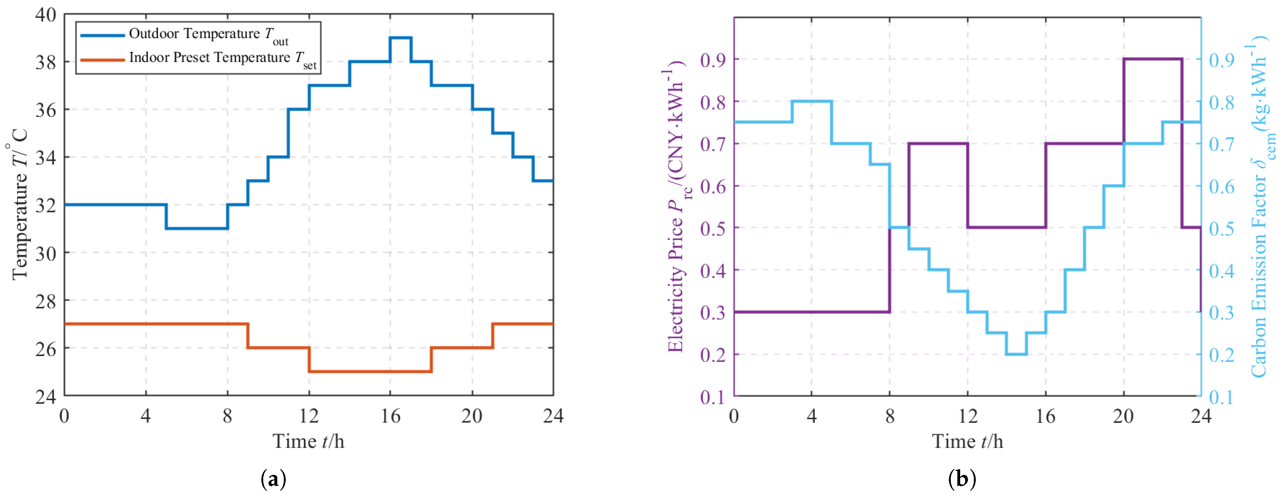
2.1. Dynamic Carbon Emission Factor

Currently, China’s average carbon emission factors face challenges, primarily due to the unification of data values at regional and provincial levels, which makes it difficult to reflect temporal and spatial variations in electric carbon factors. The numerical updates are excessively lagging, resulting in outdated information. Regional grid emission factors (e.g., average values last updated in 2012) no longer reflect real-time decarbonization progress, particularly in areas where low-carbon energy systems (e.g., photovoltaic and offshore wind) now dominate power generation portfolios [23,24]. dynamic carbon emission factors method adopted in this study utilizes a spatiotemporal grid data model. This approach couples power flow calculation results of the grid with carbon-emission correlation analysis. Time-resolved electricity carbon intensity metrics can be derived from real-time grid operational data at hourly to minute-level resolutions, supporting spatiotemporal carbon footprint quantification. In the future, dynamic carbon emission factors could be predicted in advance and released to users, allowing them to adjust electricity-consumption behaviors accordingly. Once users perceive differences in carbon-emission factors during various future periods, they could minimize carbon emissions within their adjustment capabilities. Grid carbon intensity at user nodes is governed by three determinants: (1) power flow distribution, (2) generator-specific emission coefficients, and (3) generation technology taxonomies. The load-node CEF is mathematically expressed as [25]:

$${\delta }_a={\displaystyle \frac{P_{\mathrm{g}}\times {\delta }_{\mathrm{g}}+{\sum }_{b\in {\Omega }_a}{P}_{ab}\times {\delta }_b}{P_{\mathrm{g}}+{\sum }_{b\in {\Omega }_a}{P}_{ab}}}$$

(1)

where ${\delta }_a$ and ${\delta }_b$ are the CEF at load nodes of the a-th and b-th; $P_{\mathrm{g}}$ denotes active power generation from the plant connected to node a-th; ${\delta }_g$ is the CEF of the aforementioned plant; $P_{ab}$ indicates active power transfer from node b-th to a-th through interconnecting branches; ${\Omega }_a$ represents topological set of nodes directly linked to node a-th via transmission lines.

2.2. Air Conditioning Load-Regulation Characteristics

Ambient temperature fluctuations, heat transfer properties of the building structure, real-time air conditioner system states, and device power specifications jointly determine indoor temperature variations, as captured by the following governing equations:

$$T_{\mathrm{in}}\left(t+1\right)=\left\{\begin{array}{cc}{T}_{\mathrm{out}}\left(t+1\right)-\left(T_{\mathrm{out}}\left(t+1\right)-T_{\mathrm{in}}\left(t\right)\right)e^{\frac{-\Delta t}{R_{\mathrm{rc}}{C}_{\mathrm{re}}}}\hfill & k\left(t\right)=0\hfill \\ T_{\mathrm{out}}\left(t+1\right)-\left(T_{\mathrm{out}}\left(t+1\right)-T_{\mathrm{in}}\left(t\right)-R_{\mathrm{re}}{P}_{\mathrm{e}}{\eta }_{\mathrm{cop}}\right)e^{\frac{-\Delta t}{R_{\mathrm{rc}}{C}_{\mathrm{re}}}}\hfill & k\left(t\right)=1\hfill \end{array}\right.$$

(2)

where $T_{\mathrm{in}}\left(t\right)(°\mathrm{C})$ is the indoor temperature at time t; $T_{\mathrm{out}}\left(t+1\right)\left(°\mathrm{C}\right)$ represents the outdoor temperature at time $(t+1)$; $R_{re}{(}^{°}\mathrm{C}/\mathrm{kW})$ and $C_{re}\left(\mathrm{kWh}{/}^{°}\mathrm{C}\right)$ are the equivalent thermal resistance and equivalent thermal capacitance of the indoor space respectively; $\Delta t\left(\mathrm{h}\right)$ denotes the duration of standby or working; $P\left(\mathrm{kW}\right)$ and ${\eta }_{cop}$ respectively represent the rated power and cooling energy efficiency coefficient of the air conditioning load; $k\left(t\right)=0$ and $k\left(t\right)=1$ represent the standby and operating states of the air conditioner respectively.

The optimization control technology for air conditioning loads includes automatic and direct loads control. In practical implementations, direct load control predominates, demonstrating significant advantages in reducing power consumption, lowering peak loads, and decreasin g user costs. Its operational paradigms primarily encompass intermittent cycling (on/off) and thermal setpoint adjustments [26,27].

Practically, the operational operational modes depend on two variables: binary power states (on/off) and thermal regulation modes (standby/operating) [28]. When the indoor thermal conditions fall below the threshold $T_{\min }$, the air conditioner’s switch status can remain in the “on” state while its temperature status stays in standby mode, during which the air conditioner does not cool, and the indoor temperature gradually rises. When ambient thermal conditions surpass the upper threshold $T_{\max }$, the air conditioner activates its cooling operational state, inducing a progressive reduction in indoor temperature. The indoor temperature control curves under different control modes are shown in Figure 1. Due to the direct control of air conditioning loads, the indoor temperature variation curve in Figure 1a will shift to the pattern shown in Figure 1b.

Therefore, based on the actual temperature and switch status, the operational status of the air conditioning load during the initial phase of the next time period can be determined as follows:

$$k\left(t+1\right)=\left\{\begin{array}{cc}0\hfill & u^{\mathrm{AC}}(t+1)=0\mathrm{or}{T}_{\mathrm{in}}\left(t\right)<T_{\min }\hfill \\ 1\hfill & u^{\mathrm{AC}}\left(t\right)=0\mathrm{or}{u}^{\mathrm{AC}}(t+1)=1\mathrm{and}{T}_{\mathrm{in}}\left(t\right)\ge T_{\max }\hfill \\ k\left(t\right)\hfill & u^{\mathrm{AC}}\left(t\right)=1\mathrm{and}{u}^{\mathrm{AC}}(t+1)=1\mathrm{and}{T}_{\min }\le T_{\max }\hfill \\ 1\hfill & u^{\mathrm{AC}}\left(t\right)=1\mathrm{and}{u}^{\mathrm{AC}}(t+1)=1\mathrm{and}{T}_{\mathrm{in}}\left(t\right)\ge T_{\max }\hfill \end{array}\right.$$

(3)

where $u^{\mathrm{AC}}\left(t\right)$ denotes the switch status of air conditioning load at time t; $u^{\mathrm{AC}}\left(t\right)=0$ and $u^{\mathrm{AC}}\left(t\right)=1$ respectively indicate that the air conditioner is in closed and opened states at time t.

According to the principle of indoor temperature variation in Equation (3), the turn-off and turn-on durations in Figure 1 are:

$$\begin{array}{cc}& {\theta }^{\mathrm{off}}=R_{\mathrm{re}}{C}_{\mathrm{re}}ln{\displaystyle \frac{T_{\mathrm{out}}-T_{\min }}{T_{\mathrm{out}}-T_{\max }}}\hfill \\ & {\theta }^{\mathrm{on}}=R_{\mathrm{re}}{C}_{\mathrm{re}}ln{\displaystyle \frac{R_{\mathrm{re}}{P}_{\mathrm{e}}{\eta }_{\mathrm{cop}}+T_{\max }-T_{\mathrm{out}}}{R_{\mathrm{re}}{P}_{\mathrm{e}}{\eta }_{\mathrm{cop}}+T_{\min }-T_{\mathrm{out}}}}\hfill \end{array}$$

(4)

where ${\theta }^{\mathrm{off}}$ and ${\theta }^{\mathrm{on}}$ represent the durations of being closed and opened, respectively.

3. Optimization Objectives and Constraints for Air Conditioning Day-Ahead Scheduling

This study proposes a multi-objective air conditioning loads scheduling framework to enhance thermal comfort satisfaction and optimize economic-environmental trade-offs. Accounting for heterogeneous thermal preference constraints across users, the day-ahead optimization model integrates the following objectives:

$$\begin{array}{cc}& min{f}_1=\sum _{z=1}^{\mathrm{Z}}\sum _{s=1}^{\mathrm{S}}{\omega }_z\left(t\right)\times \left|T_z^{\mathrm{avg}}\left(t\right)-T_z^{\mathrm{set}}\left(t\right)\right|\hfill \\ & min{f}_2=\sum _{z=1}^{\mathrm{Z}}\sum _{s=1}^{\mathrm{S}}{u}_z^{\mathrm{AC}}\times \Delta t\times P_e\times \left[{\psi }_e\left(t\right)+{\sigma }_z\left(t\right)\times {\psi }_c\left(t\right)\right]\hfill \end{array}$$

(5)

$$\left\{\begin{array}{c}{u}_z^{\mathrm{AC}}\left(t\right)\in \{0,1\};\hfill \\ n=1,2,\dots ,Z;\hfill \\ t=1,2,\dots ,\mathrm{S};\hfill \\ Z=4;\hfill \\ \mathrm{S}=24\hfill \end{array}\right.$$

(6)

where $f_1$ is defined as the temperature comfort deviation function; $f_2$ is formulated as a multi-criteria energy expenditure function, integrating power cost and carbon emissions; Z denotes the consumers count; ${\omega }_z\left(t\right)$ denotes the weight of indoor temperature demand for the z-th consumer at time t; $T_z^{\mathrm{avg}}\left(t\right)$ and $T_z^{\mathrm{set}}\left(t\right)$ represent the average indoor temperature and preset indoor temperature for the z-th consumers at time t respectively; $u_z^{\mathrm{AC}}$ represents the on/off status of the air conditioning load for the z-th consumers; $\Delta t\left(\mathrm{h}\right)$ indicates the duration of operation for the z-th consumers at time t; $P_{\mathit{e}}$ represents the rated power of consumers air conditioning loads; $\mathrm{S}\left(h\right)$ represents the number of hours in a day; ${\sigma }_z\left(t\right)$ represents the carbon emission factor of electricity for the z-th consumers at time t, calculated via Equation (1) based on real-time grid power flow ($P_{ab}$), generator emission coefficients (${\delta }_g$), and renewable energy penetration ${\psi }_e\left(t\right)$ and ${\psi }_c\left(t\right)$ represent the electricity price and carbon price at time t respectively. The binary state $u_z^{\mathrm{AC}}\left(t\right)\in \{0,1\}$ follows the operational logic in Equation (3): off (0) if $T_{\mathrm{in}}\left(t\right)<T_{\min }$ or manual shutdown, on (1) if $T_{\mathrm{in}}\left(t\right)\ge T_{\max }$.

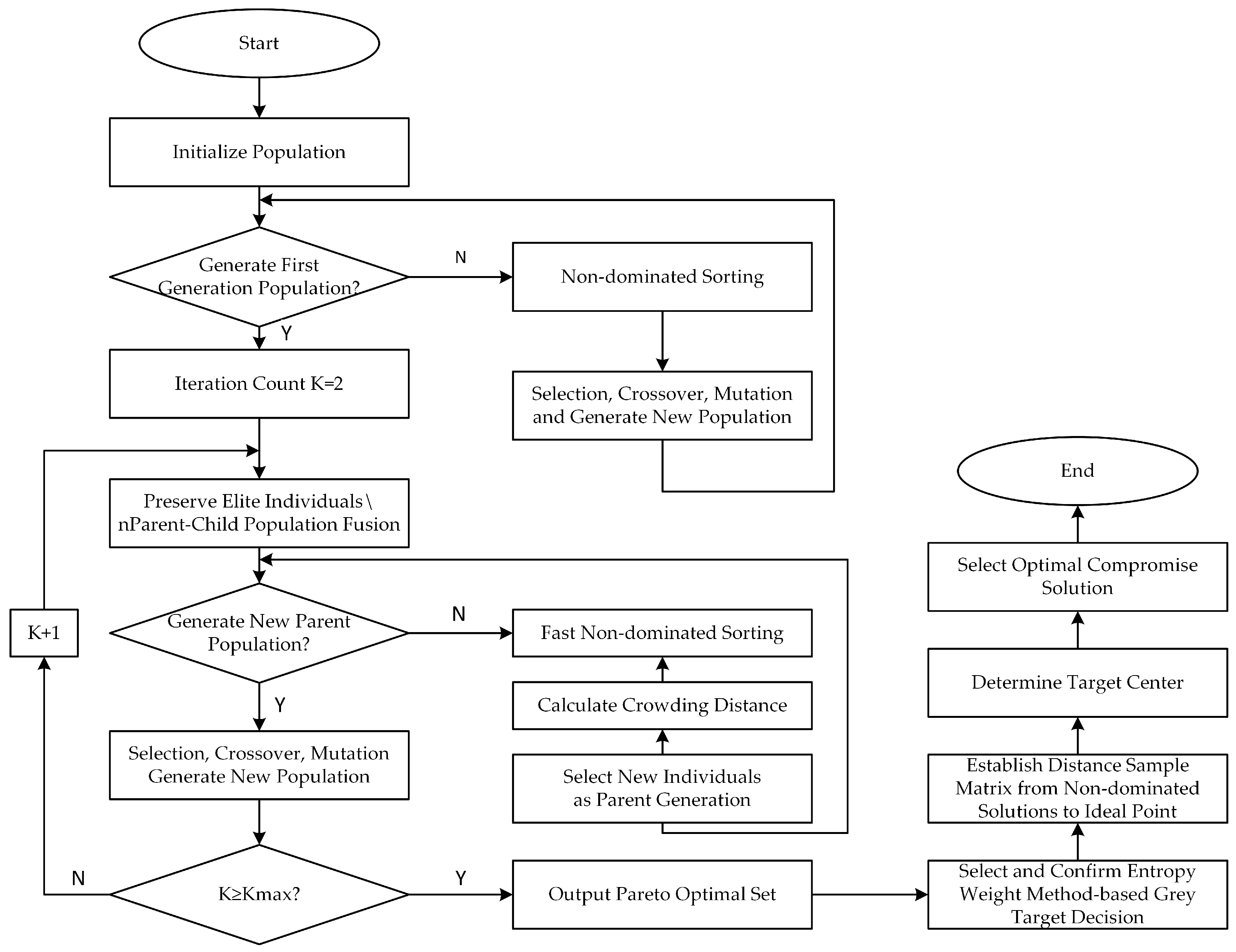
4. NSGA-II and Grey Target Decision-Making Combined Optimal Day-Ahead Scheduling of Air Conditioning Loads

4.1. NSGA-II

NSGA-II is a dominance-based multi-objective optimization algorithm [29]. NSGA-II is essentially a genetic algorithm but differs from ordinary GA [30] in two aspects: (1) non-dominated sorting, and (2) the calculation of crowding distance and the crowding-distance-based elitist preservation strategy.

4.1.1. Non-Dominated Sorting

Assume there exists a population. First, select the pareto front as the highest dominance level (rank 1). After removing rank 1 solutions, select the current pareto front from the remaining population, which exhibits secondary dominance compared to rank 1, denoted as rank 2. Subsequently, eliminate rank 2 solutions and repeat this process to identify new pareto fronts in the residual population. This cyclic procedure continues until the population is fully stratified, where solutions of higher ranks can dominate those of lower ranks, thereby completing the comprehensive non-dominated sorting.

4.1.2. Crowding Distanceg

Taking the bi-objective problem as an example, assume there exists a solution h. The perimeter of the matrix shape formed by its adjacent solutions $h-1$ and $h+1$ is defined as the crowding distance. When calculating crowding distance, only solution h is permitted within the formed rectangular area. The magnitude of a solution’s crowding distance characterizes the sparsity around it—smaller crowding distances indicate narrower solution coverage, which is detrimental to population diversity. Therefore, solutions with larger crowding distances are preferentially selected. The fundamental principle of the NSGA-II algorithm can be summarized as [31]:

(1)

Suppose there is a population $P_r$. First, use the selection, crossover and mutation operators of the GA algorithm to obtain the offspring $Q_r$ with the same number of individuals as the population $P_r$, then combine the two to get a new group, denoted as $R_r$. Then, carry out non-dominated sorting for $R_r$ to obtain each domination level, such as $1,2,3\dots$

(2)

According to the obtained domination level order, sequentially add individuals from the high domination level to the low domination level into the next population $P_{r+1}$.

(3)

When the number of optimal solutions in a certain domination level is too large and exceeds the capacity of $P_{r+1}$, sort all individuals of this level according to the crowding distance, retain the individuals with larger crowding distances and add them to the population $P_{r+1}$ first, until the population $P_{r+1}$ is full.

4.2. Grey Target Decision-Making

A hybrid entropy-weighted grey target decision framework is proposed to objectively identify pareto-optimal equilibrium solutions from NSGA-II-generated non-dominated sets, eliminating human preference bias in multi-criteria optimization. The implementation framework comprises the following sequential phases:

(1)

Based on the normalized pareto solution set and the distances from each non-dominated solution to the ideal point, establish the sample matrix.

(2)

Normalize the sample matrix to obtain the decision matrix, and determine the bullseye within the grey decision region formed by the decision matrix.

(3)

Calculate all distances to the bullseye.

4.2.1. Establish Sample Matrix

Based on the pareto optimal solution set obtained by the NSGA-II algorithm, m decision-making methods can be derived. Each decision-making method contains n objectives, where the j-th objective value in the i-th decision-making method is defined as an element of the newly constructed sample matrix [27]. This element is denoted as $x_i\left(j\right)(i=1,2,\dots ,m;j=1,2,\dots ,n)$, and the sample matrix is expressed as $X={\left[x_i\left(j\right)\right]}_{m\times n}$. The specific solving method is as follows:

$$X={\left[\begin{array}{c}{x}_i\left(j\right)\end{array}\right]}_{m\times n}=X_{min}+{\displaystyle \frac{x_i\left(j\right)-x{\left(j\right)}_{min}}{x{\left(j\right)}_{max}-x{\left(j\right)}_{min}}}(X_{max}-X_{min})$$

(7)

$$X={\left[\begin{array}{c}{x}_i\left(j\right)\end{array}\right]}_{m\times n}=\left[\begin{array}{cccc}{x}_1\left(1\right)& x_1\left(2\right)& \dots & x_1\left(n\right)\\ x_2\left(1\right)& x_2\left(2\right)& \dots & x_2\left(n\right)\\ \dots & \dots & \dots & \dots \\ x_m\left(1\right)& x_m\left(2\right)& \dots & x_m\left(n\right)\end{array}\right]$$

(8)

where $X_{\max }$, $X_{\min }$ denote the upper and lower bounds of the normalized fitness function domain; $x{\left(j\right)}_{max}$, $x{\left(j\right)}_{min}$ represent the extremal objective function values for the j-th pareto-optimal solution; X comprises a composite matrix of standardized fitness metrics across all candidate solutions.

4.2.2. Determine the Bullseye

The target value is selected as a cost-type indicator:

$$y_i\left(j\right)={\displaystyle \frac{w\left(j\right)-x_i\left(j\right)}{max\{{max}_{1\le i\le m}{x}_i\left(j\right)-w\left(j\right),w\left(j\right)-{min}_{1\le i\le m}{x}_i\left(j\right)}}$$

(9)

where $w\left(j\right)$ represents the average value of each column in the sample matrix.

$$w\left(j\right)={\displaystyle \frac{{\sum }_{i=1}^m{x}_i\left(j\right)}{m}}$$

(10)

Accordingly, the decision matrix $Y=y_i\left(j\right)(i=1,2,\dots ,m;j=1,2,\dots ,n)$ is constructed. The bullseye vector is then formulated by extracting the maximum value from each column of Y, resulting in:

$$y_o=\{y{\left(1\right)}_{max},\dots ,y{\left(j\right)}_{max},\dots ,y{\left(n\right)}_{max}\}$$

(11)

where $y{\left(j\right)}_{max}$ denotes the highest attainable value for the j-th objective function.

4.2.3. Select the Best Compromise Solution

The optimal compromise solution is determined through grey target modeling integrated with entropy weighting [32], and the calculation method is employed to determine the weights. The steps are as follows:

(1)

Calculate the weight value $t_i\left(j\right)$ of the j-th objective for the i-th decision alternative

$$t_i\left(j\right)={\displaystyle \frac{x_i\left(j\right)}{{\sum }_{i=1}^m{x}_i\left(j\right)}},x_i\left(j\right)>0$$

(12)

(2)

Calculate the entropy value $E\left(j\right)$ of the j-th objective value for the i-th decision alternative

$$E\left(j\right)=-{\displaystyle \frac{{\sum }_{i=1}^m{t}_i\left(j\right)ln{t}_i\left(j\right)}{lnm}},E\left(j\right)>0$$

(13)

(3)

Calculate the entropy weight $p\left(j\right)$ of the j-th objective value

$$\begin{array}{cc}\hfill p\left(j\right)& ={\displaystyle \frac{1-E\left(j\right)}{{\sum }_{j=1}^n(1-E\left(j\right))}},p\left(j\right)>0\hfill \end{array}$$

(14)

(4)

Calculate the distance from each solution to the bullseye, and select the solution closest to the bullseye as the optimal decision-making solution.

$$d_i=\mid y_i-y_o\mid =\sum _{i=1}^n{\omega }_j\left|y_i\left(j\right)-y_o\right|$$

(15)

4.3. Mathematical Expressions

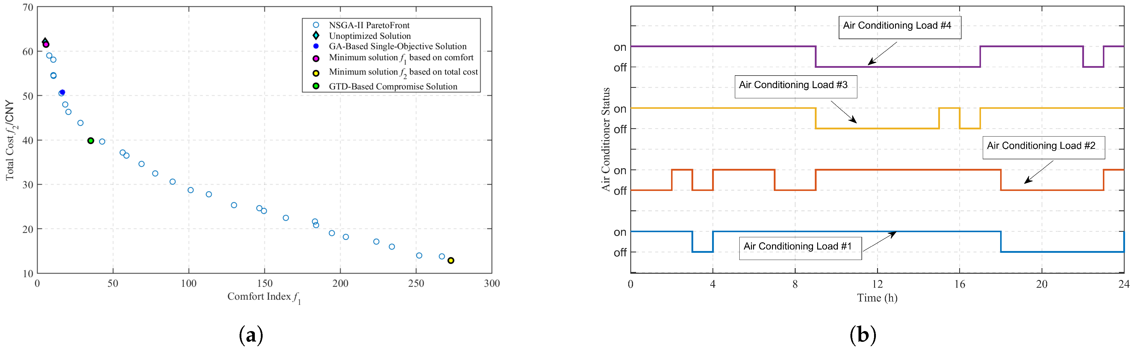
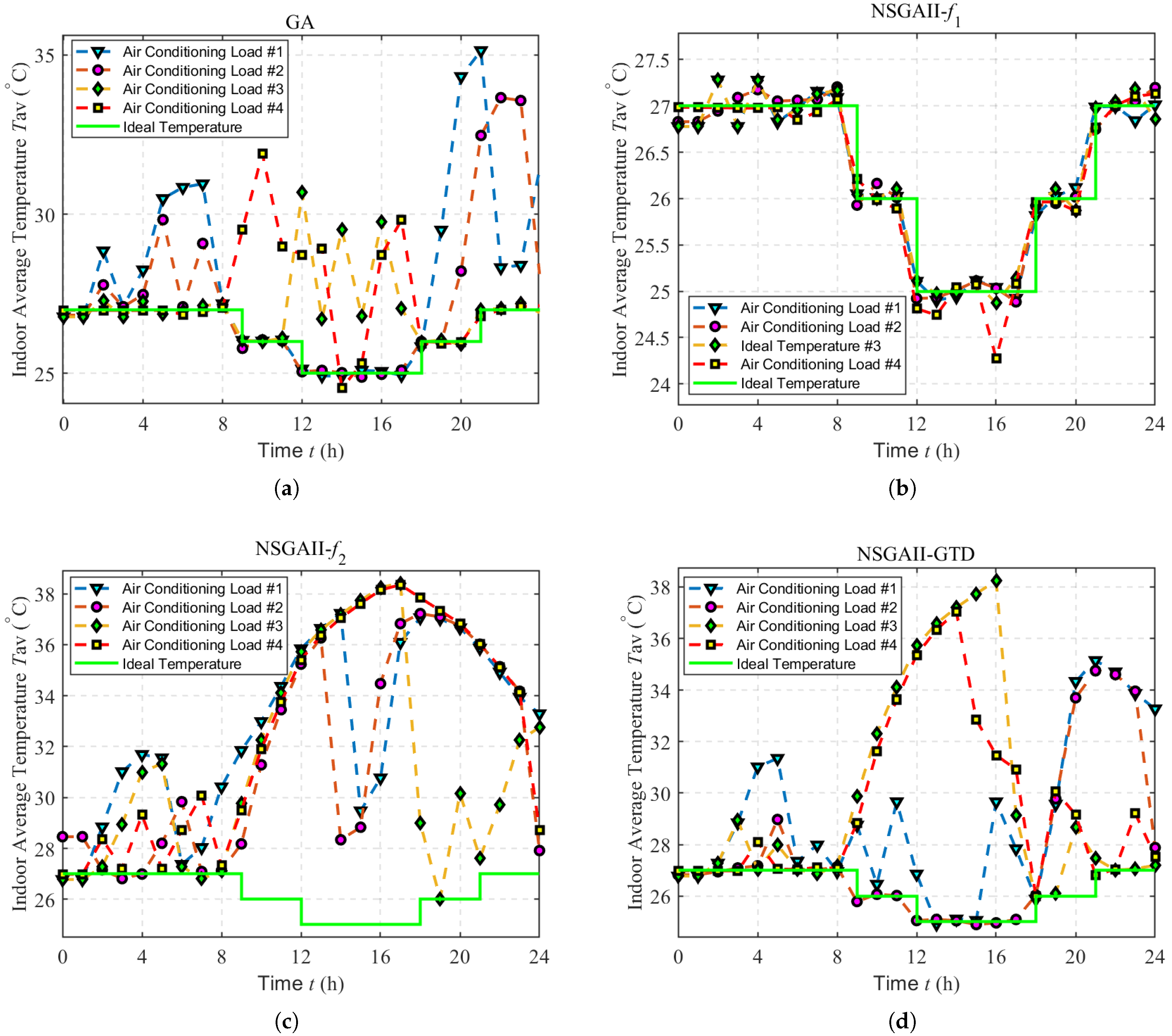
In summary, the algorithm flow combining NSGA-II and grey target decision-making is shown in Figure 2.

5. Case Study

To verify the effectiveness and universality of the proposed optimization strategy, four air conditioning loads with different usage habits are set, and their main parameters and temperature control periods are shown in

Table 1. Main parameters and temperature control periods of 4 air conditioning loads.

Air Conditioning Load Number	R (°C/kW)	C (kWh/°C)	P (kW)	${\mathit{\eta }}_{\mathit{cop}}$	Temperature Control Period
#1	5.36	0.16	4.0	1.1	09:00–18:00
#2	6.00	0.19	3.5	1.5	09:00–18:00
#3	5.60	0.16	2.5	2.0	00:00–08:00, 18:00–24:00
#4	5.76	0.19	2.3	1.2	00:00–08:00, 18:00–24:00

. Referring to references [33,34], from which the time and location information is also referenced,

Table 2. Twenty-four-hour dynamic carbon emission factor numerical table.

Cases	Time (hours)	Dynamic CEF (kgCO2/kWh)
#1	00:00–12:00	0.75	0.75	0.80	0.80	0.70	0.70	0.65	0.50	0.45	0.40	0.35	0.30
	12:00–24:00	0.25	0.20	0.25	0.30	0.40	0.50	0.60	0.70	0.70	0.75	0.75	0.80
#2	00:00–12:00	0.99	1.00	0.99	0.99	0.99	0.99	0.99	0.97	0.97	0.96	0.93	0.96
	12:00–24:00	0.96	0.96	0.97	0.98	0.96	0.96	0.97	0.97	0.97	0.97	1.00	0.99

statistics the dynamic CEF values at each moment of 24 h. Figure 3 shows the outdoor temperature, indoor preset temperature, time-of-use electricity price, and dynamic CEF in 24 h a day. Among them, during the day, the proportion of power generation from renewable energy sources (such as solar power generation) is relatively large, resulting in a smaller value of the electricity carbon factor. On the contrary, the proportion of power generation from renewable energy sources at night is relatively low. The unavailability of photovoltaic output after sunset necessitates increased reliance on thermal power infrastructure (e.g., coal plants) for baseline electricity provision. Consequently, the dynamic CEF exhibits a characteristic diurnal pattern, with carbon intensity troughs during daylight hours and peaks under night-time load conditions. In addition, the single-objective optimization based on GA, and the multi-objective optimizations based on NSGAI-II-$f_1$ and NSGA-II-$f_2$ are used as comparison strategies to comprehensively analyze the superiority of the NSGA-II-GTD strategy. To achieve a fair comparison, the maximum number of iterations and population size of GA and NSGA-II are completely the same, with the maximum number of iterations $K_{\max }=200$ and the population size $Pop=100$.

Figure 4a shows the pareto front obtained by NSGA-II and the optimal solutions under different optimization strategies. It can be seen that the un-optimized and GA-based single-objective solutions are close in position, both near the vertical axis, with the maximum total cost. This indicates that these two strategies are similar to the NSGA-II-$f_1$-based optimization strategy, favoring the best comfort but neglecting the cost-optimization objective. Conversely, the solution based on the minimum cost $f_2$ is closer to the horizontal axis, with the maximum comfort index $f_1$, obtaining the minimum total cost at the expense of user comfort. Obviously, the above-mentioned strategies cannot simultaneously take into account the two optimization objectives of comfort and cost, and it is difficult to win user favor. In contrast, the trade-off solution obtained by GTD can well balance the two objectives, ensuring that users are in relatively comfortable conditions while reducing the total cost, which better aligns with user expectations. The optimal scheduling strategy based on NSGA-II-GTD is shown in Figure 4b. Air conditioners #1 and #2 remain in the on state from 09:00 to 18:00, while air conditioners #3 and #4 are primarily active from 00:00 to 08:00 and 18:00 to 24:00. This operational pattern precisely corresponds to the temperature-control periods, further verifying the scientific validity of the proposed strategy.

Table 3. Comparison of optimization indexes of four air conditioning loads based on different optimization strategies.

AC Load No.	Index	Optimization Strategy
		Unoptimized	GA	NSGAII-${\mathit{f}}_{\mathbf{1}}$	NSGAII-${\mathit{f}}_{\mathbf{2}}$	MOEA/D-GTD	NSGAII-GTD
#1	Electricity Cost (dynamic CEF)	19.5599	15.0625	20.0199	3.5798	11.6337	13.1902
	Carbon Cost (dynamic CEF)	0.8161	0.5039	0.8461	0.5565	0.3916	0.5565
	Carbon Cost (average CEF)	1.0303	0.6774	1.0303	0.5840	0.6439	0.5840
	Total Cost (dynamic CEF)	20.3760	15.5664	20.8660	4.1363	12.0253	13.7467
	Comfort Index (dynamic CEF)	0.9453	5.3550	0.9554	84.2978	12.3692	7.6286
#2	Electricity Cost (dynamic CEF)	12.9610	11.1824	12.9732	3.2835	8.3983	9.1371
	Carbon Cost (dynamic CEF)	0.5356	0.4127	0.5424	0.3830	0.3122	0.3830
	Carbon Cost (average CEF)	0.6774	0.5624	0.6774	0.4550	0.4697	0.4552
	Total Cost (dynamic CEF)	13.4966	11.5951	13.5156	3.6665	8.7106	9.5201
	Comfort Index (dynamic CEF)	0.8877	2.9321	0.8912	75.7282	9.3734	6.7590
#3	Electricity Cost (dynamic CEF)	10.2313	8.8882	10.4920	3.2523	8.1771	6.9628
	Carbon Cost (dynamic CEF)	0.4233	0.3953	0.5216	0.3402	0.3409	0.3402
	Carbon Cost (average CEF)	0.5374	0.4767	0.5286	0.4376	0.4215	0.4376
	Total Cost (dynamic CEF)	10.6546	9.2835	11.0136	3.5925	8.5180	7.3030
	Comfort Index (dynamic CEF)	2.2436	4.0547	2.3766	37.0784	9.3383	7.8487
#4	Electricity Cost (dynamic CEF)	16.8213	13.7174	16.3060	1.9716	12.0848	8.7775
	Carbon Cost (dynamic CEF)	0.6859	0.6076	0.6763	0.4877	0.5314	0.4877
	Carbon Cost (average CEF)	0.8804	0.6949	0.8804	0.4526	0.5926	0.4526
	Total Cost (dynamic CEF)	17.5072	14.3250	16.9823	2.4593	12.6163	9.2652
	Comfort Index (dynamic CEF)	1.2312	4.2892	1.7640	75.7444	10.0666	13.1019
Total Load	Electricity Cost (dynamic CEF)	59.5735	48.8505	59.7911	12.0872	40.2939	38.0676
	Carbon Cost (dynamic CEF)	2.4609	1.9195	2.5864	1.7674	1.5761	1.7674
	Carbon Cost (average CEF)	3.1255	2.4114	3.1167	1.9292	2.1277	1.9294
	Total Cost (dynamic CEF)	62.0344	50.7700	62.3775	13.8546	41.8701	39.8350
	Comfort Index (dynamic CEF)	5.3078	16.6310	5.9872	272.8488	41.1475	35.3382

All costs are in Chinese yuan (CNY). China’s 2024 average carbon price (CNY 91.80/ton CO₂). For reference, the 2024 EU ETS carbon price averaged EUR 68.00/ton CO₂ ≈ CNY 534.48/ton at EUR 1 = CNY 7.86). Carbon markets in China and the EU operate under independent pricing mechanisms.

summarizes optimization metrics for four air conditioning loads under dynamic carbon emission factor scenarios, including power-consumption cost, carbon emission cost, total cost, and comfort indices. The bolded values indicate optimal performance. Using Jiangxi’s 2020 provincial grid average emission factor ($0.616{\mathrm{kgCO}}_2/\mathrm{kWh}$) from “Research on China’s Regional Grid Carbon Dioxide Emission Factors (2023)” as baseline, both GA-based single-objective optimization and NSGA-II-GTD strategies achieve cost reductions while maintaining acceptable comfort levels. However, single-objective optimization demonstrates limitations in flexibility and universality due to its unified objective framework. The NSGA-II-GTD strategy emerges as the preferred approach for obtaining compromise solutions in air conditioning load day-ahead scheduling. Specifically, this strategy reduces carbon-emission costs by 12.05% compared to average emission factor scenarios, and decreases total costs by 21.5% versus GA-based optimization. The NSGA-II-GTD algorithm demonstrates superior balance between global and local search capabilities. Comparative analysis reveals MSCSO-GTD achieves the lowest carbon emission costs while satisfying both comfort requirements and total cost optimization. This algorithm exhibits rapid convergence and high precision, effectively maintaining equilibrium between exploration and exploitation in solution space.

Figure 5 presents the average temperature-variation curves for four air conditioning loads under different optimization strategies. Influenced by the comfort index, minor deviations in average indoor temperature occur during temperature-control periods, while larger deviations manifest in non-temperature-control periods. Similar temperature trends emerge between air conditioning loads #1/#2 and #3/#4 due to shared temperature-control schedules. Comparative analysis reveals consistent performance patterns across optimization strategies: The NSGA-II-$f_2$ strategy demonstrates the poorest temperature control, with maximum deviations exceeding $13°\mathrm{C}$. Unoptimized and NSGA-II-$f_1$ strategies produce temperature curves closest to the ideal trajectory, maintaining deviations within ±1.5 °C—indicative of superior temperature-regulation capability and optimal comfort. The MOEA/D-GTD approach shows intermediate temperature-regulation performance, though its total cost (CNY 41.87) and comfort index (41.15) in total load evaluation are both inferior to NSGAII-GTD (CNY 39.84 and 35.34 respectively). The NSGA-II-GTD strategy achieves effective control during temperature-regulation periods, limiting maximum temperature differences below 3 °C while satisfying basic user requirements.

Figure 6 shows a comparison chart of the costs and comfort levels of each air conditioning load under different optimization strategies. Overall, the application effects of different optimization strategies on each air conditioning load are similar. The higher the comfort level, the higher the cost; the power-consumption cost is the main component of the total cost. The optimization indicators of air conditioning loads #1–3 obtained by the NSGA-II-$f_1$ strategy are identical to those without optimization, and only the cost of air conditioning load #4 has slightly decreased. This indicates that the optimization capability of NSGA-II-$f_1$ is highly limited. NSGA-II-$f_2$ achieves the minimum cost, but its comfort indicator fails to meet requirements. The minimum comfort indicator exceeds 35, resulting in poor user experience. Although the GA-based single-objective optimization strategy has a slightly lower comfort level than the NSGA-II-GTD strategy, its cost is 10.94 yuan higher than the latter, rendering it uneconomical. Furthermore, under the NSGA-II-GTD strategy, the comfort indicators of all air conditioning loads remain below 15, fully satisfying user comfort requirements. This further demonstrates the superiority and coordination of the proposed strategy.

6. Conclusions

In view of the current dilemmas of traditional air conditioners, such as incomplete consideration of day-ahead scheduling optimization objectives and outdated optimization strategies, this paper incorporates carbon emission costs based on dynamic carbon emission factors into optimization objectives alongside electricity cost reduction and user comfort improvement. A multi-objective day-ahead scheduling strategy for air conditioner loads using NSGA-II-GTD is proposed. Through simulation analysis, three key conclusions emerge:

(1)

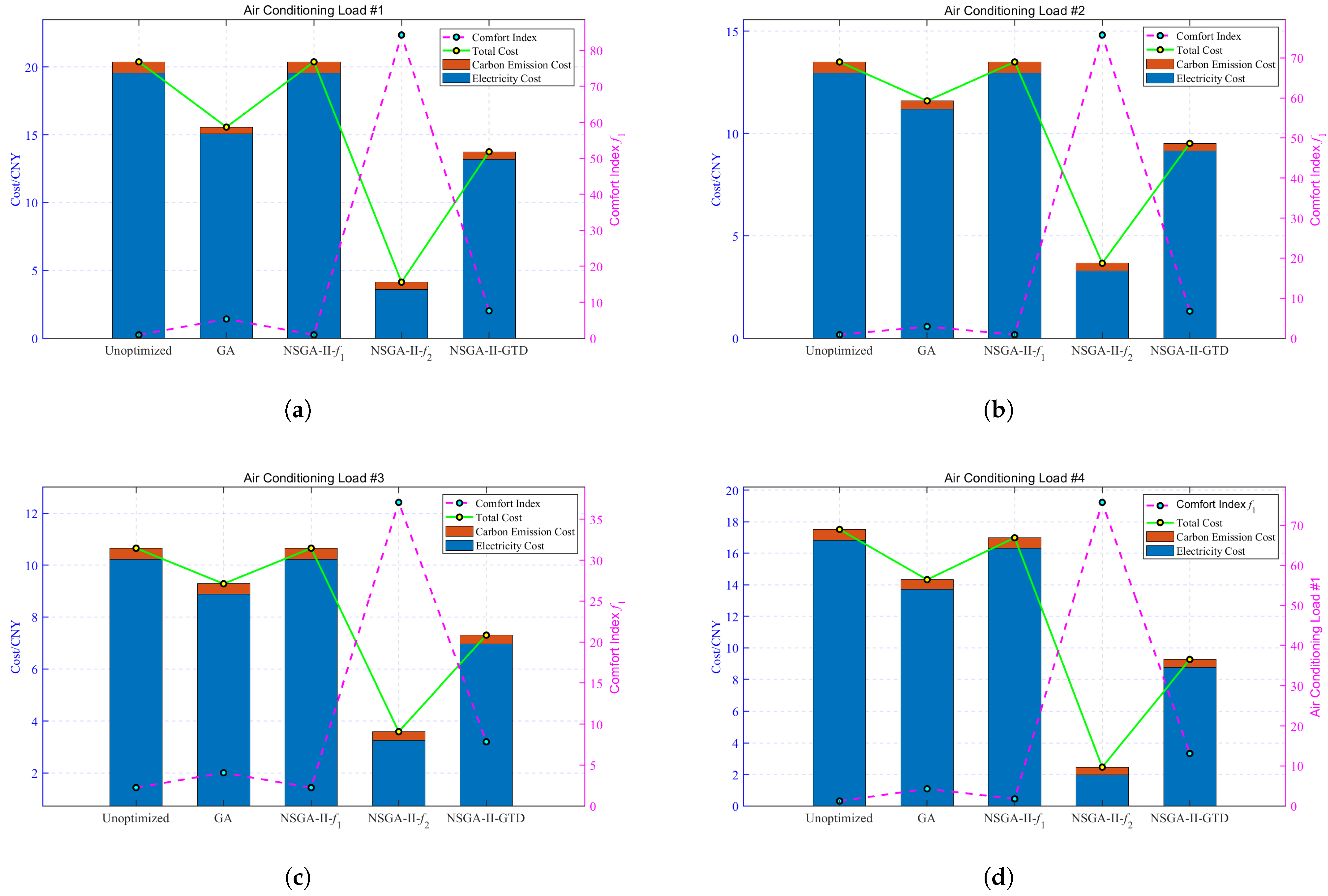
User costs and comfort exhibit inherent conflict. The pareto frontier obtained by NSGA-II shows that when prioritizing comfort entirely, the temperature deviation remains below 1.5 °C, but the cost reaches 62 CNY. Conversely, when focusing solely on cost reduction, the maximum temperature deviation exceeds 13 °C. These results demonstrate that the two objectives cannot be minimized simultaneously, adhering to the "no free lunch" theorem.

(2)

NSGA-II-GTD proves operationally effective. Compared to competitive strategies (GA, NSGA-II-$f_1$, or NSGA-II-$f_2$), the proposed NSGA-II-GTD method achieves a balanced solution, reducing electricity costs by 36.09% (from 59.57 to 38.07 CNY) and carbon-emission costs by 28.05% (from 2.46 to 1.77 CNY) while maintaining comfort deviations below 15 for all users (vs. 272.85 for NSGA-II-$f_2$).

While the current study has demonstrated the effectiveness of the proposed strategy in cooling scenarios, its potential applicability to heating operations warrants further investigation. Future work should address heating-mode optimization, where low PV yield and grid dependency may require hybrid energy models. Seasonal adaptation of comfort constraints and emission factors will be critical.

References

1. Möller, T.; Högner, A.E.; Schleussner, C.F.; Bien, S.; Kitzmann, N.H.; Lamboll, R.D.; Rogelj, J.; Donges, J.F.; Rockström, J.; Wunderling, N. Achieving net zero greenhouse gas emissions critical to limit climate tipping risks. Nat. Commun. 2024, 15, 6192. [Google Scholar] [CrossRef] [PubMed]
2. Cao, J.; Dai, H.; Li, S.; Guo, C.; Ho, M.; Cai, W.; He, J.; Huang, H.; Li, J.; Liu, Y.; et al. The general equilibrium impacts of carbon tax policy in China: A multi-model comparison. Energy Econ. 2021, 99, 105284. [Google Scholar] [CrossRef]
3. Mengesha, I.; Roy, D. Carbon pricing drives critical transition to green growth. Nat. Commun. 2025, 16, 1321. [Google Scholar] [CrossRef] [PubMed]
4. Liu, Q.; Mao, C.; Tian, F. Influencing Factors of CO2 Emissions in Chinese Power Industry: A Study from the Production and Consumption Perspectives. Comput. Intell. Neurosci. 2022, 2022, 3615492. [Google Scholar] [CrossRef]
5. Guo, Y.; Li, H.; Pan, M. Colocation Data Center Demand Response Using Nash Bargaining Theory. IEEE Trans. Smart Grid 2018, 9, 4017–4026. [Google Scholar] [CrossRef]
6. Zeng, X.; Zhang, Y.; Guo, B.; Huang, L.; Li, C. Optimal Day-Ahead Dispatch of Air-Conditioning Load under Dynamic Carbon Emission Factors. In Proceedings of the 2023 5th Asia Energy and Electrical Engineering Symposium (AEEES), Chengdu, China, 23–26 March 2023; pp. 1–6. [Google Scholar] [CrossRef]
7. Algarni, A.S.; Suryanarayanan, S.; Siegel, H.J.; Maciejewski, A.A. Combined Impact of Demand Response Aggregators and Carbon Taxation on Emissions Reduction in Electric Power Systems. IEEE Trans. Smart Grid 2021, 12, 1825–1827. [Google Scholar] [CrossRef]
8. Fleschutz, M.; Bohlayer, M.; Braun, M.; Henze, G.; Murphy, M.D. The Effect of Price-Based Demand Response on Carbon Emissions in European Electricity Markets: The Importance of Adequate Carbon Prices. Appl. Energy 2021, 295, 117040. [Google Scholar] [CrossRef]
9. Wang, Y.; Qiu, J.; Tao, Y. Robust Energy Systems Scheduling Considering Uncertainties and Demand Side Emission Impacts. Energy 2022, 239, 122317. [Google Scholar] [CrossRef]
10. Agrawal, K.K.; Jain, S.; Jain, A.K.; Dahiya, S. Assessment of Greenhouse Gas Emissions from Coal and Natural Gas Thermal Power Plants Using Life Cycle Approach. Int. J. Environ. Sci. Technol. 2014, 11, 1157–1164. [Google Scholar] [CrossRef]
11. Ma, W.; Cai, D.; Wan, L.; Chen, R.; Liu, H.; Cao, K. A Calculation Method of Dynamic Carbon Emission Factors for Different Regions in a Province Based on Time Division. In Proceedings of the 2023 Panda Forum on Power and Energy (PandaFPE), Chengdu, China, 27–30 April 2023; pp. 963–967. [Google Scholar] [CrossRef]
12. Zhu, S.; Wang, E.; Han, S.; Ji, H. Optimal Scheduling of Combined Heat and Power Systems Integrating Hydropower-Wind-Photovoltaic-Thermal-Battery Considering Carbon Trading. IEEE Access 2024, 12, 98393–98406. [Google Scholar] [CrossRef]
13. Li, J.; Wenjing, C.; Ying, X.; Miao, B.; Na, M. The Calculation Method of User-Level Dynamic Carbon Emission Factor Based on Electric Energy Trading Flow. In Proceedings of the 2023 IEEE 5th International Conference on Power, Intelligent Computing and Systems (ICPICS), Shenyang, China, 14–16 July 2023; pp. 374–379. [Google Scholar] [CrossRef]
14. Tan, H.; Yu, H.; Chen, T.; Qiao, W. Research on Carbon Emission Monitoring Indicator System of Power Users. In Proceedings of the 2023 IEEE/IAS Industrial and Commercial Power System Asia (I&CPS Asia), Chongqing, China, 7–9 July 2023; pp. 613–619. [Google Scholar] [CrossRef]
15. Zhang, S.; Li, Y.; Du, E.; Wang, W.; Wang, M.; Feng, H.; Xie, Y.; Chen, Q. Research on Carbon-Reduction-Oriented Demand Response Technology Based on Generalized Nodal Carbon Emission Flow Theory. Energies 2024, 17, 4672. [Google Scholar] [CrossRef]
16. Zhang, Q.; Qiao, K.; Hu, C.; Su, P.; Cheng, O.; Yan, N.; Yan, L. Study on Life-Cycle Carbon Emission Factors of Electricity in China. Int. J. Low-Carbon Technol. 2024, 19, 2287–2298. [Google Scholar] [CrossRef]
17. Gao, P.; Li, B.; Yan, C.; Li, D.; Huang, Y.; Yang, X.; Li, K.; Wu, D. Multi-Objective Coordinated Optimal Scheduling Considering Electric Vehicles and Air-conditioning Loads (CICED 2024). In Proceedings of the 2024 China International Conference on Electricity Distribution (CICED), Hangzhou, China, 12–13 September 2024; pp. 235–240. [Google Scholar] [CrossRef]
18. Deb, K.; Pratap, A.; Agarwal, S.; Meyarivan, T. A Fast and Elitist Multiobjective Genetic Algorithm: NSGA-II. IEEE Trans. Evol. Comput. 2002, 6, 182–197. [Google Scholar] [CrossRef]
19. Li, R.; Jiang, Z.; Ji, C.; Li, A.; Yu, S. An Improved Risk-Benefit Collaborative Grey Target Decision Model and Its Application in the Decision Making of Load Adjustment Schemes. Energy 2018, 156, 387–400. [Google Scholar] [CrossRef]
20. Zhang, G.; Yan, Y.; Zhang, K.; Li, P.; Li, M.; He, Q.; Chao, H. Time-of-Use Pricing Model Considering Wind Power Uncertainty. CSEE J. Power Energy Syst. 2022, 8, 1039–1047. [Google Scholar] [CrossRef]
21. Guo, S.; Kurban, A.; He, Y.; Wu, F.; Pei, H.; Song, G. Multi-Objective Sizing of Solar-Wind-Hydro Hybrid Power System with Doubled Energy Storages Under Optimal Coordinated Operational Strategy. CSEE J. Power Energy Syst. 2023, 9, 2144–2155. [Google Scholar] [CrossRef]
22. Mahdi, B.S.; Sulaiman, N.; Shehab, M.A.; Shafie, S.; Hizam, H.; Hassan, S.L.B.M. Optimization of Operating Cost and Energy Consumption in a Smart Grid. IEEE Access 2024, 12, 18837–18850. [Google Scholar] [CrossRef]
23. Elenes, A.G.N.; Williams, E.; Hittinger, E.; Goteti, N.S. How Well Do Emission Factors Approximate Emission Changes from Electricity System Models? Environ. Sci. Technol. 2022, 56, 14701–14712. [Google Scholar] [CrossRef]
24. Xiong, T.; Liu, Y.; Yang, C.; Cheng, Q.; Lin, S. Research Overview of Urban Carbon Emission Measurement and Future Prospect for GHG Monitoring Network. Energy Rep. 2023, 9, 231–242. [Google Scholar] [CrossRef]
25. Yang, C.; Liu, J.; Liao, H.; Liang, G.; Zhao, J. An Improved Carbon Emission Flow Method for the Power Grid with Prosumers. Energy Rep. 2023, 9, 114–121. [Google Scholar] [CrossRef]
26. Zhu, G.X.; Bao, Y.Q.; Yu, Q.Q. A Control Strategy for Air-Conditioning Loads Participating in Frequency Regulation Based on Model Predictive Control. Sustain. Energy Grids Netw. 2024, 38, 101369. [Google Scholar] [CrossRef]
27. Callaway, D.S.; Hiskens, I.A. Achieving Controllability of Electric Loads. Proc. IEEE 2011, 99, 184–199. [Google Scholar] [CrossRef]
28. Li, W.; Wu, H.; Zhao, Y.; Jiang, C.; Zhang, J. Study on Indoor Temperature Optimal Control of Air-Conditioning Based on Twin Delayed Deep Deterministic Policy Gradient Algorithm. Energy Build. 2024, 317, 114420. [Google Scholar] [CrossRef]
29. Duan, L.; Guo, Z.; Taylor, G.; Lai, C.S. Multi-Objective Optimization for Solar-Hydrogen-Battery-Integrated Electric Vehicle Charging Stations with Energy Exchange. Electronics 2023, 12, 4149. [Google Scholar] [CrossRef]
30. Shojae Chaeikar, S.; Mirzaei Asl, F.; Yazdanpanah, S.; Zamani, M.; Manaf, A.A.; Khodadadi, T. Secure CAPTCHA by Genetic Algorithm (GA) and Multi-Layer Perceptron (MLP). Electronics 2023, 12, 4084. [Google Scholar] [CrossRef]
31. Ma, H.; Zhang, Y.; Sun, S.; Liu, T.; Shan, Y. A Comprehensive Survey on NSGA-II for Multi-Objective Optimization and Applications. Artif. Intell. Rev. 2023, 56, 15217–15270. [Google Scholar] [CrossRef]
32. Zu, X.; Yang, C.; Wang, H.; Wang, Y. An EGR Performance Evaluation and Decision-Making Approach Based on Grey Theory and Grey Entropy Analysis. PLoS ONE 2018, 13, e0191626. [Google Scholar] [CrossRef]
33. Zhang, X.; Guo, Z.; Pan, F.; Yang, Y.; Li, C. Dynamic Carbon Emission Factor Based Interactive Control of Distribution Network by a Generalized Regression Neural Network Assisted Optimization. Energy 2023, 283, 129132. [Google Scholar] [CrossRef]
34. Wang, J.; Jin, X.; Jia, H.; Tostado-Véliz, M.; Mu, Y.; Yu, X.; Liang, S. Joint Electricity and Carbon Sharing With PV and Energy Storage: A Low-Carbon DR-Based Game Theoretic Approach. IEEE Trans. Sustain. Energy 2024, 15, 2703–2717. [Google Scholar] [CrossRef]
Figure 1. Room indoor temperature variation curves under different control modes of air conditioning load. (a) Automatic control. (b) Direct control.
Electronics 14 01550 g001
Figure 2. Algorithm flow combining NSGA-II and grey target decision.
Electronics 14 01550 g002
Figure 3. Preset conditions. (a) Outdoor temperature and indoor preset temperature. (b) Electricity price and dynamic carbon emission factor.
Electronics 14 01550 g003
Figure 4. Comparison of optimization objectives and typical air conditioning scheduling strategies. (a) Comparison of optimization indexes under different optimization strategies. (b) NSGA-II-GTD based air conditioning scheduling strategy.
Electronics 14 01550 g004
Figure 5. Variation curves of average indoor temperature for each air conditioning load under different optimization strategies. (a) GA. (b) NSGAII- f 1 . (c) NSGAII- f 2 . (d) NSGAII-GTD.
Electronics 14 01550 g005
Figure 6. Comparison diagrams of cost and comfort for each air conditioning load under different optimization strategies. (a) Air conditioner load #1. (b) Air conditioner load #2. (c) Air conditioner load #3. (d) Air conditioner load #4.
Electronics 14 01550 g006