Article

An RF Fingerprinting Blind Identification Method Based on Deep Clustering for IoMT Security

1
School of Information and Software Engineering, University of Electronic Science and Technology of China, Chengdu 610054, China
2
Tianfu Jiangxi Laboratory, Chengdu 641419, China
3
The Affiliated Stomatological Hospital of Chongqing Medical University, Chongqing 401147, China
4
College of Software, Xinjiang University, Urumqi 830046, China
*
Author to whom correspondence should be addressed.
Electronics 2025, 14(8), 1504; https://doi.org/10.3390/electronics14081504
Submission received: 5 March 2025 / Revised: 1 April 2025 / Accepted: 3 April 2025 / Published: 9 April 2025

Abstract

:
To tackle the issue of unknown spoofing attacks in the Internet of Medical Things (IoMT), we put forward an iterative deep clustering model for blind RF fingerprint recognition. This model seamlessly combines a representation learning module and a clustering module, facilitating end—to—end training and optimization. Its parameters are updated according to an innovative loss function. Moreover, this model incorporates a noise—canceling self—encoder module to reduce noise and extract the noise—independent intrinsic fingerprints of devices. In comparison with other algorithms, the proposed model remarkably improves the blind recognition performance for the identification of unknown devices in the IoMT.

1. Introduction

The Internet of Medical Things (IoMT) has witnessed remarkable development in recent years, leading to a substantial increase in the number of radio-frequency (RF) medical devices. Conventionally, communication security in the IoMT relies on user passwords, encryption algorithms, and various network communication protocols [1]. However, this makes it vulnerable to network spoofing attacks such as eavesdropping, monitoring, and replay.

1.1. Motivation

In IoMT systems, the application of traditional complex cryptographic algorithms is indeed restricted on medical sensor nodes with limited resources. Due to the constraints on the computational power and storage capacity in medical sensor nodes, which are typically micro-embedded systems, the direct application of complex cryptographic algorithms may encounter performance bottlenecks or resource exhaustion issues. Therefore, it is necessary to propose a secure authentication method that does not require computational resources. Medical devices possess unique hardware-specific differences that are difficult to replicate. Even within the same device class, subtle variations occur in their internal components during manufacturing and usage. By analyzing and extracting these inherent differences, RF fingerprinting features can be obtained. These features are distinct and remain stable within the short term [1], making them suitable for device identification. Moreover, RF fingerprinting identification operates at the physical layer, offering a potential solution to the problem of spoofing attacks in the IoMT [2].
To handle unknown spoofing attacks with limited samples for model training, traditional clustering methods have been applied to RF fingerprinting identification. Nevertheless, in a typical medical environment, RF signals are exposed to complex factors such as noise, channel fading, and interference [3]. Facing these complex signals, traditional identification methods encounter numerous issues, including high computational complexity, ineffective dimensionality reduction, poor noise resistance, and suboptimal clustering performance. As a result, traditional machine-learning-based clustering methods cannot be effectively applied in RF fingerprinting for the IoMT [4].
In recent years, due to the automatic feature extraction capabilities and the ability to approximate complex functions in deep learning, its combination with clustering tasks has attracted extensive attention, and research on deep clustering has emerged [5]. The success of deep clustering depends on an effective sample representation. The learned features should not only be a low-dimensional approximation of the original samples but also capture the structural characteristics of the original samples to a large extent, thus achieving a better clustering effect.
Existing deep clustering methods all rely on deep neural networks to perform representation learning on samples and then cluster according to the results of the representation learning. According to the interaction mode between the representation learning module and the clustering module, the existing deep clustering methods can be summarized into the following four branches [6].
(1)
Multi-stage deep clustering methods
In this type of method, the representation learning module and the clustering module are connected sequentially. This type of method first uses deep unsupervised representation learning techniques to learn the representation of each data instance, and then feeds the learned representation back into a classic clustering model to obtain the final clustering result. This method of separating data processing and clustering is convenient in enabling researchers to conduct clustering analyses, and this method has strong universality and can be applied to almost all research scenarios. The authors in [6] trained a deep autoencoder to learn the representations of samples, and these representations could be directly input into k-means for clustering.
Multi-stage deep clustering methods have advantages such as programming friendliness and intuitive principles. However, this simple combination of deep representation learning and traditional machine learning clustering often cannot achieve the optimal result [7]. Firstly, most representation learning methods are not specifically designed for clustering tasks, which leads to the fact that the learned sample representations may not necessarily achieve good clustering results. Secondly, due to the characteristic of the separation of the two stages, the clustering result cannot be used in reverse to guide the representation learning module to enable the representation module to obtain better data representations. Therefore, this direct module cascade cuts off the information interaction between representation learning and clustering, so the limitations of either side will jointly affect the final performance, resulting in the algorithm only being able to achieve suboptimal clustering results.
(2)
Iterative deep clustering methods
Aiming at the limitations of multi-stage deep clustering methods, iterative deep clustering methods allow the clustering results to guide the representation learning in reverse. Generally speaking, the clustering module in deep iterative clustering will generate pseudo-labels, which can be used to train the representation learning module in a supervised manner. DeepCluster [8] is a representative and mature deep iterative clustering method that has achieved success in the fields of image clustering and video clustering [2]. DeepCluster alternately updates between the backbone representation module and the k-means clustering module by minimizing the gap between the clustering assignment predicted by the representation learning module and the pseudo-labels, and it can achieve better clustering results.
The method of deep iterative clustering enables representation learning and clustering to promote each other. However, at the same time, they are also affected by error propagation during the iterative process. Especially in the early stage of training, inaccurate clustering results may cause the representation learning module to generate confused representations, and these representations will in turn affect the clustering results, ultimately resulting in the model not being able to achieve the expected effect or even being unable to train and converge.
(3)
Parallel deep clustering methods
Although the iterative deep clustering method allows the information between the representation learning module and the clustering module to guide them, these two modules are optimized in an explicit, iterative manner and they cannot be updated simultaneously. In the parallel deep clustering method, the representation learning module and the clustering module are optimized simultaneously in an end-to-end manner. DEC [3] is a representative method that combines the autoencoder with the self-training strategy to optimize clustering and representation learning simultaneously, and this idea has had a profound impact on subsequent research. The authors in [4] introduced an additional noise encoder and improved the robustness of the autoencoder by minimizing the reconstruction error of each layer between the noise decoder and the original encoder. The authors in [5] applied the self-training method between the original branch and the enhanced branch, further improving the robustness of clustering. The authors in [9] improved the distribution of the target by increasing the normalized frequency of the clusters, solved the problems of data imbalance and uneven sample distribution, and could maintain the distinguishability of small groups.
Contrastive learning has been one of the most popular unsupervised representation learning techniques in recent years, and its basic idea is to pull positive instance pairs closer and push negative instance pairs farther apart. The representative method of contrastive clustering is CC [10], whose basic idea is to construct positive and negative sample pairs, regard each cluster as a data instance in the low-dimensional space, minimize the distance between similar samples, and maximize the distance between different samples. There are also some variants based on CC. PICA [11] directly separates different clusters by minimizing the cosine similarity between the statistical vectors assigned by clusters, and DRC [12] introduces a regularization method for the clusters of clustering.
(4)
Generative deep clustering methods
Generative deep clustering can be further divided into methods based on variational autoencoders (VAEs) and methods based on generative adversarial networks (GANs). The VAE is a probabilistic model based on variational inference, and the model is trained by assuming the distribution of latent variables. The VAE has led to many models, including GMVAE [13], VaDE [14], etc. Generative adversarial networks (GANs) have achieved great success in the field of computer vision and in the estimation of complex data distributions. In recent years, there have also been studies applying GANs to deep clustering. The authors in [15] proposed stacking a Gaussian mixture model (GMM) with a GAN, using the GMM as the prior distribution for the generation of data instances. The authors in [16] proposed directly replacing the GMM with a GAN and proposed a new method to solve the convergence problem in the early stage of the model. The authors in [17] proposed using the Sobel operation before the discriminator of the GAN to improve the model performance.
Although deep generative clustering models can generate samples while completing clustering, they also have some disadvantages. Firstly, the training of generative models usually involves Monte Carlo sampling, which may lead to unstable training and high computational complexity. Secondly, VAE-based models usually require prior assumptions about the data distribution, but this may not be applicable in actual situations; while GAN-based algorithms are more flexible and diverse, they may encounter problems such as mode collapse and slow convergence speeds. In summary, there are still several problems in the research of radio-frequency (RF) fingerprints.
Most of the existing research regards RF fingerprint recognition as a supervised task that requires the manual annotation of the collected RF signals in advance to form a dataset. However, the actual electromagnetic environment is often complex and changeable. When facing a complex electromagnetic environment, it is not always feasible to collect data in advance and construct a dataset through manual annotation. This requires the participation of industry experts, which is quite difficult and incurs high human and time costs. Moreover, the effect of manual annotation directly affects the subsequent recognition effect. In addition, when facing some specific types of network attacks, such as spoofing attacks and Sybil attacks, these supervised methods often fail due to the appearance of unknown devices, while unsupervised blind recognition methods can effectively prevent such attacks.
In the actual electromagnetic environment, multipath noise will be introduced into the signals, and the subtle differences between different devices of the same model are not easy to detect, making it difficult to extract and recognize RF fingerprints. Most of the existing research methods on RF fingerprints has been carried out in ideal scenarios. The constructed models are easily affected by the characteristics of the electromagnetic environment, leading to the overfitting or degradation of the models, which has led to a disconnect between theoretical research and practical applications.

1.2. Contributions

This paper presents an iterative deep clustering model to solve the problem of RF fingerprint blind identification in an IoMT environment. By borrowing the idea of the clustering module, we propose a Collaborative Denoising Autoencoder and Data Classifier (CDAE-DC) model. This method is designed under the architecture of the representation learning module but does not require the labeling of samples, meaning that it can be widely used in real applications. Moreover, we design a noise-reducing autoencoder module in this method, which can denoise highly noisy inphase/quadrature (I/Q) signals, minimize the impact of noise, extract the noise-independent intrinsic fingerprints of devices, and improve the blind identification performance.
The rest of this paper is organized as follows. Section 2 describes the background of the IoMT. Section 3 presents the method of CDAE-DC based on deep iterative clustering. Section 4 and Section 5 present the experimental design and the analysis of the results, respectively. Section 6 concludes with a discussion of the results and suggestions for future research.

2. Background of IoMT

The Internet of Medical Things integrates technologies such as telemedicine, the Internet, the Internet of Things, automatic control, and artificial intelligence. It is a comprehensive system for the all-round operation and management of medical institutions, aiming to enhance medical quality, reduce medical errors, improve patient service levels, and optimize the overall operational efficiency.

2.1. Typical Business Scenarios in the Internet of Medical Things

There are four typical business scenarios in the Internet of Medical Things [9].
  • Smart Clinical Scenarios for Medical Staff
Smart clinical scenarios are mainly designed for nurses. The integration of mobile intelligent terminals and wireless communication technology enables nurses to access patients’ admission information, vital signs, surgical data, and examination information accurately and in real time during ward services. This improves the efficiency and quality of ward rounds.
2.
Smart Patient Services for Patients
Smart patient services are mainly targeted at special or critically ill patients in the hospital. These services include in-hospital navigation, personnel positioning, and emergency alarm functions. Through smart wearable bracelets and RFID tags, the intelligent monitoring system can track a patient’s walking route and real-time location. If the patient leaves the restricted area, an alarm will be triggered, and medical staff can promptly assist the patient in returning to a safe area to prevent accidents.
Additionally, when a patient suddenly feels unwell and needs urgent help, they can use the smart wearable device to send a one-click alarm. Medical staff can then respond quickly to ensure the patient’s safety.
3.
Smart Management for Medical Institution Management
The scale of modern hospital campuses is expanding rapidly, and the number and types of hospital assets have also increased significantly. Traditional asset management methods can no longer meet the management needs of hospitals. The smart management model based on the Internet of Things technology can significantly improve the level of hospital asset management.
Using RFID technology, when purchasing equipment assets, an entry registration is created to generate an asset ledger, which is then transmitted to the asset comprehensive management platform via the WiFi network. The entire life cycle of assets, including allocation, use, change, recovery, inventory, and scrapping, can be tracked and managed, achieving refined, standardized, and professional asset management to adapt to the rapid growth of hospital business.
4.
Remote Health Management for Communities
During the implementation of public health services, due to factors such as the increasing number of people covered by medical institutions and the imbalance in regional medical resources, it is difficult to conduct health screening in all areas in a timely manner. Community self-service terminals using 5G technology can perform health screening at the doorstep.
Health parameter detection data, such as height, weight, fat percentage, water ratio, blood oxygen, blood pressure, and electrocardiogram data, are transmitted to the back-end analysis system of the medical institution via the 5G network. The central end uniformly evaluates and analyzes the examination results and provides suggestions. This simplifies and streamlines the work of front-line medical staff and enables the public to benefit from the inclusive policies of China’s public health services. Remote health management is an important part of the “Internet hospital” construction. Through the Internet of Things and 5G technology, it connects front-line rural doctors and outpatient experts from large-scale tertiary hospitals, realizing the universal sharing of medical resources and bringing the benefits of modern technology to the people.
The application of the Internet of Medical Things permeates all aspects of the medical industry. Most hospitals in China have a certain informatization foundation through the Hospital Information Management System (HIS). However, issues such as the inability to synchronously enter medical information in a timely manner and the relatively independent information interactions between different departments still exist. The construction of smart hospitals enables the integration and interaction of massive data from networked medical devices, mobile client devices, remote nursing systems, interconnected clinical information systems, security monitoring systems, and medical research data. The Internet of Things technology can break the information silos between departments, enabling hospitals to conduct comprehensive data collection and use big data analysis to improve the efficiency and refine the operational management of the entire medical institution, thereby enhancing the overall informatization level and diagnosis and treatment service capabilities.

2.2. Network Security Issues Faced by the Internet of Medical Things

In the medical field, commonly used IoT tools include a series of external devices, such as infusion pumps and patient monitoring systems, and wirelessly connected implanted devices, such as cardiac defibrillators, pacemakers, and prosthetics. While these devices bring a better treatment experience to patients, they also expand the attack surface of the network and increase the security risks [10].
  • Attacks on Implanted Devices
In 2012, in the second season of the American TV series Homeland, hackers accessed the pacemaker of the Vice President of the United States. They sent a high-current command to the pacemaker, ultimately causing the Vice President’s death. After this episode was broadcast, the medical team of then US Vice President Dick Cheney disabled the wireless function of his pacemaker due to concerns about potential hacker attacks.
At that time, this might have appeared merely as a fictional story. However, in 2017, the US Food and Drug Administration (FDA) issued a notice recalling 465,000 wireless radio-frequency implanted pacemakers. Their review found that hackers could change the program, potentially harming patients by depleting the battery or increasing the pacemaker’s speed [18].
In March 2019, the US Department of Homeland Security warned that the cardiac defibrillators produced by the medical technology company Medtronic had serious flaws. Hackers could fully control these devices through radio communication after they were implanted in patients, endangering the patient’s life without being detected [19].
2.
Attacks on External Devices
In 2016, a security vulnerability was discovered in the Owlet baby heart monitoring sensor in the UK. Researchers found that, although the data transmission between the parents’ smartphones and the base server was secure, the network between the sensor and the base server had no encryption and could be accessed without logging in. This meant that anyone within the monitoring range could monitor the baby’s data, interfere with the alarm system, or disrupt the monitoring [20].
Infusion pumps that deliver drugs into a patient’s bloodstream are also vulnerable to hacker attacks. A white-hat hacker claimed to have written a program that could remotely control the infusion pump to deliver a lethal dose of drugs to the patient. Although the infusion pump had a firewall, it could be easily disabled.
In addition, security personnel found that hackers could intercept the signals of blood glucose monitors and change the readings, which might lead the wearer to adjust the dosage incorrectly. A recent study by the security company McAfee also shows that hackers can easily tamper with the vital signs of patients monitored by computers.

3. Method of CDAE-DC Based on Deep Iterative Clustering

To address the challenge of unknown spoofing attacks in the Internet of Medical Things (IoMT), we propose an iterative deep clustering model for blind RF fingerprint recognition.

3.1. Overall Structure of the CDAE-DC Model

The structure of the CDAE-DC model is illustrated in Figure 1. The overall network loss consists of two components: classification loss and reconstruction loss. When calculating the classification loss, the model adopts an iterative clustering algorithm that supports end-to-end training. Soft labels are generated through the clustering algorithm, based on which the classification loss is computed [21].
The update of the network parameters guides the model and improves the clustering performance. To enhance the model’s ability to extract fingerprints from highly noisy samples, CDAE-DC also introduces the reconstruction loss. Essentially, this can be regarded as a convolutional denoising autoencoder (CDA) [12]. CDAE-DC first enhances the original I/Q samples through a channel model; it then learns the inherent fingerprint features of the samples via an encoder and finally decodes and reconstructs these features. The difference between the original and the reconstructed features forms the reconstruction error. The classification error, based on the clustering results, guides the update of the network parameters, training the network to optimize the clustering performance. The reconstruction error guides the network to extract noise-independent features, enhancing the model’s noise robustness. The classification error and the reconstruction error together constitute the total network error, which improves the clustering effect while enhancing the model’s robustness. The CDAE-DC model can be described algorithmically as shown in Algorithm 1.
Algorithm 1 Iterative clustering algorithm.
Input: dataset D, total training rounds E (epochs), batch size of each batch N, number of categories M
Output: Class cluster assignment result
Training Phase:
1: for epoch = i to E do:
2: mini-batch { x i } i = 1 N from dataset D;
3: Add noise to the sample: x i a = T x i ;
4: Extract the features of the enhanced sample by encoding: h = f x i a ;
5: Perform PCA dimensionality reduction and clustering on sample features to obtain pseudo-labels:
P s e u d o   l a b l e s = c P C A h
6: Calculate the classification loss L C from (5);
7: Decoding the feature map by the decoder: x ~ = d h ;
8: Calculate the reconstruction loss L r from (8);
9: Calculate the total loss L from (10);
10: Gradient descent algorithm minimizes contrast loss L and updates the parameters of the entire network, i.e., f · , g · d · ;
11: end for
Test Phase:
1: for x in D  do:
2: Extract features by encoder: h = f x
3: Compute class cluster assignment l: l = g h
4: end for

3.2. Calculation of Classification Loss

To extract the noise-independent intrinsic fingerprints of devices, the CDAE-DC model first introduces random perturbations to the input I/Q samples, mainly by simulating different channels [13]. In this study, the additive Gaussian white noise channel (AWGN) is selected to modify the original samples. For a stationary signal X t , t T for arbitrary t + τ , t T , we have
R τ = N 0 δ t 2 ,       S ω = N 0 2
where R · is the autocorrelation function, and S · represents the power spectrum. Additive Gaussian white noise is a stationary stochastic process with a constant power spectral S · density. For input I/Q samples x, the above process can be expressed as
x _ a = H ( x )
Subsequently, x a is fed into the encoder f · for fingerprint feature extraction, and the feature map h is obtained as
h = f _ θ   ( x _ a )
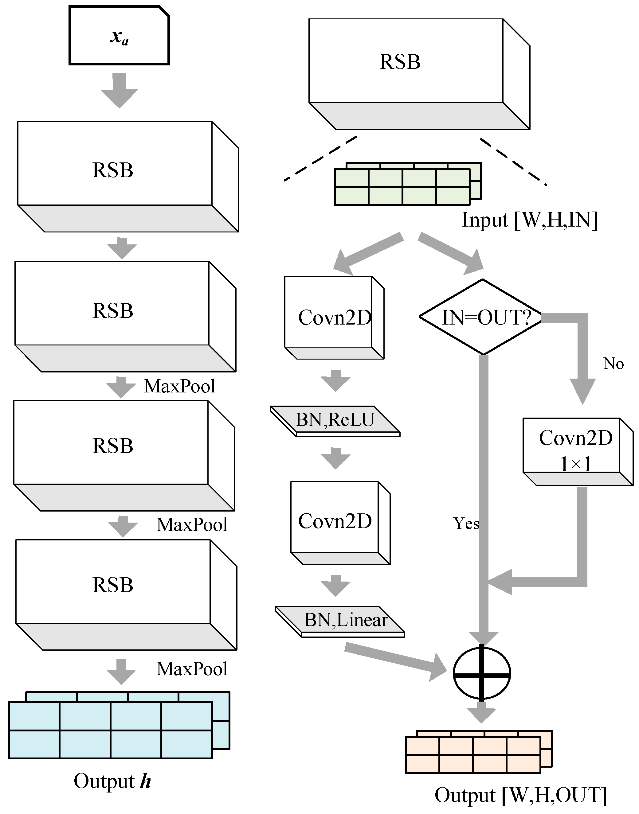
where f θ · represents the encoder network, and θ represents the encoder network parameters. The encoder part of CDAE-DC is designed based on residual networks. When the CNN reaches a certain depth, increasing the number of layers does not result in the expected further increase in accuracy, which makes the model difficult to train and even unable to converge. The residual network uses cross-layer connections, which can facilitate backpropagation and update the network parameters more efficiently through identity mapping. Moreover, it can prevent related problems in gradient propagation caused by a large number of layers in the network, making the training of deep networks possible. The encoder structure of CDAE-DC is shown in Figure 2.
The encoder of CDAE-DC consists of four stacked residual blocks (RSB), and the structure of the RSBs is illustrated in Figure 2. Each RSB can be divided into a direct mapping part and a residual part, and its output feature map is composed of these two parts [14]. In the residual part, two convolution operations are performed on the input feature map, followed by a batch normalization operation. The batch normalization operation in the middle layer of the CNN can, to some extent, prevent overfitting during training and accelerate the model’s convergence. The output after the two convolutions is activated using the Rectified Linear Unit (ReLU) activation function. During the convolution operation, the number of channels in the feature map can be adjusted, resulting in a difference in the dimensions of the input and output feature maps. Since the outputs of the residual part and the direct mapping part cannot be directly added, a 1 × 1 convolutional layer is inserted into the direct mapping part to match the number of channels in the input feature map with that of the output from the residual part. The detailed structure of the CDAE-DC encoder is presented in Table 1.
CDAE-DC uses the k-means algorithm as its clustering algorithm. The clustering process begins with the initialization of cluster centers, which can be randomly selected or chosen according to specific rules. Based on the distance calculation rule, other samples are assigned to the nearest cluster. After the sample assignment process is completed, the cluster center is updated according to the samples within the cluster. This process is repeated until the sum of the squared errors between each sample and its cluster center is minimized. The loss function can be expressed as
min C R d × k 1 N n = 1 N m i n f θ x n C y n 2 2 ,       y n 0,1 k y n T I k = 1
where f θ x n represents the features extracted by the encoder from sample x n , θ is the encoder parameter, matrix C represents the coordinates of cluster center k, and y n is the pseudo-label generated by clustering.
After the clustering process, CDAE-DC treats the clustering results as pseudo-labels and then trains the encoder and classifier in a supervised learning manner. Therefore, the classification loss can be expressed as
L c = min θ , W 1 N n = 1 N l g W f θ x n , y n
where θ and W represent the network parameters of the encoder f ( · ) and classifier g ( · ) , respectively. l is the softmax function. The softmax function is a commonly used classification loss function in deep learning, and it can be expressed as
s o f t m a x x i = e x i j = 0 n e x j
In (6), a particularly large x j in the input can lead to a large value of e x j , resulting in the overflow of the softmax function. When each element in the input is a very small negative number, j = 0 n e x j becomes extremely small, resulting in the underflow of the softmax function. Thus, in (6), the selected log-softmax function solves the possible overflow and underflow problems.
The construction of the CDAE-DC classification loss involves an alternating process: using (4) for clustering to generate pseudo-labels and then using (5) to calculate the classification loss. The classification loss is part of the total network loss and guides the update of the overall network parameters through the gradient descent method. However, this alternating clustering and network updating approach may lead to trivial solutions in the model, resulting in meaningless outcomes.

3.3. Calculation of Reconstruction Loss

To enhance the model’s anti-noise performance, the reconstruction loss is incorporated into the overall loss of CDAE-DC [15]. Moreover, in order to recover the original data from the feature map h extracted by the encoder, we need to design a decoder that is characterized by using an upsampling process. The structure of the decoder is shown in Table 2.
The decoding process of the decoder can be represented as
x ~ = d ( h )
In (7), x ~ is the output generated by the decoder’s reconstruction. Thus, the reconstruction loss can be expressed as
L _ r = M S E ( x , x ~ ) x ~ = d ( h )
where M S E · represents the mean squared error, which is one of the loss functions for regression problems and is defined as
M S E y , y ~ = 1 n i = 1 n y i y i ~ 2 L _ r = M S E ( x , x ~ ) x ~ = d ( h )
Therefore, the total error of CDAE-DC is
L = L c + L r

4. Experimental Design

This experiment was conducted on a Dell T640 server (Dell Technologies Inc., Round Rock, TX, USA), and the detailed hardware configuration of the server is presented in Table 3.
The experiment was developed, trained, and tested in a Linux environment, mainly relying on software such as Python v3.6.5 and MATLAB R2018a. The Keras and Tensorflow frameworks were utilized to build and train the model, as shown in Table 4.

4.1. Data Collection

To evaluate the performance of the proposed deep clustering models, we used a real-world dataset (generated by the USRP). The real-world dataset used in this study contains raw I/Q data from 8 USRP devices in the laboratory. The number of I/Q samples is shown in Table 5.
The devices are USRP devices, which are manufactured by Ettus Research, a subsidiary of National Instruments. USRP X410 is based on a Xilinx Zynq Ultrascale+ RFSOC ZU28DR, which can operate in the 7 GHz band and is suitable for applications requiring a high frequency and wide bandwidth. The USRP X410 has strong flexibility and expansibility in communication standards and protocols. It can not only support the current mainstream 5G NR standard, but also be well integrated with open-source development frameworks. In this study, we selected the 5G NR standard as the communications standard.
The detailed procedures used to collect the real-world signals are as follows. (1) Signal specification and parameter configuration: (a) frequency range—we determine the frequency range of the real-world signals to collect; we use the USRP software vX410 interface to set the center frequency as 2.4 GHz and the bandwidth as 15 MHz; (b) sampling rate—the sampling rate is set to be twice the highest frequency component of the signal according to the Nyquist–Shannon sampling theorem, and thus we set the sampling rate to 30 M samples per second. (2) Signal collection: (a) initialization—we start the USRP software and initialize it using the appropriate software commands; this involves setting up the radio parameters and configuring the data flow from the USRP to the host computer; (b) recording—we use a data recording tool to start capturing the received signals; this is a simple file writer block that saves the sampled signal data to a file on the host computer; the data are usually saved in a format that can be easily processed later, such as a binary file; (c) monitoring—while the signals are being collected, we use various visualization tools to monitor the received signal; this includes spectrum analyzers, time-domain plotters, etc., which allow us to observe the characteristics of the signals in real time and ensure that the collection process is working as expected. (3) Data post-processing and analysis: (a) data retrieval—once the signal collection is complete, we retrieve the recorded data from the host computer; this involves copying the data file to a different location or format for further processing; (b) signal processing—we use appropriate signal processing algorithms and tools to analyze the collected data; this includes techniques such as filtering, demodulation, and decoding depending on the type of signal; (c) data visualization—we visualize the processed data to gain insights into the characteristics of the real-world signals; this is achieved by using plotting libraries in Python v3.6.5. We create graphs showing the frequency spectrum, time-domain waveforms, or other relevant signal features.
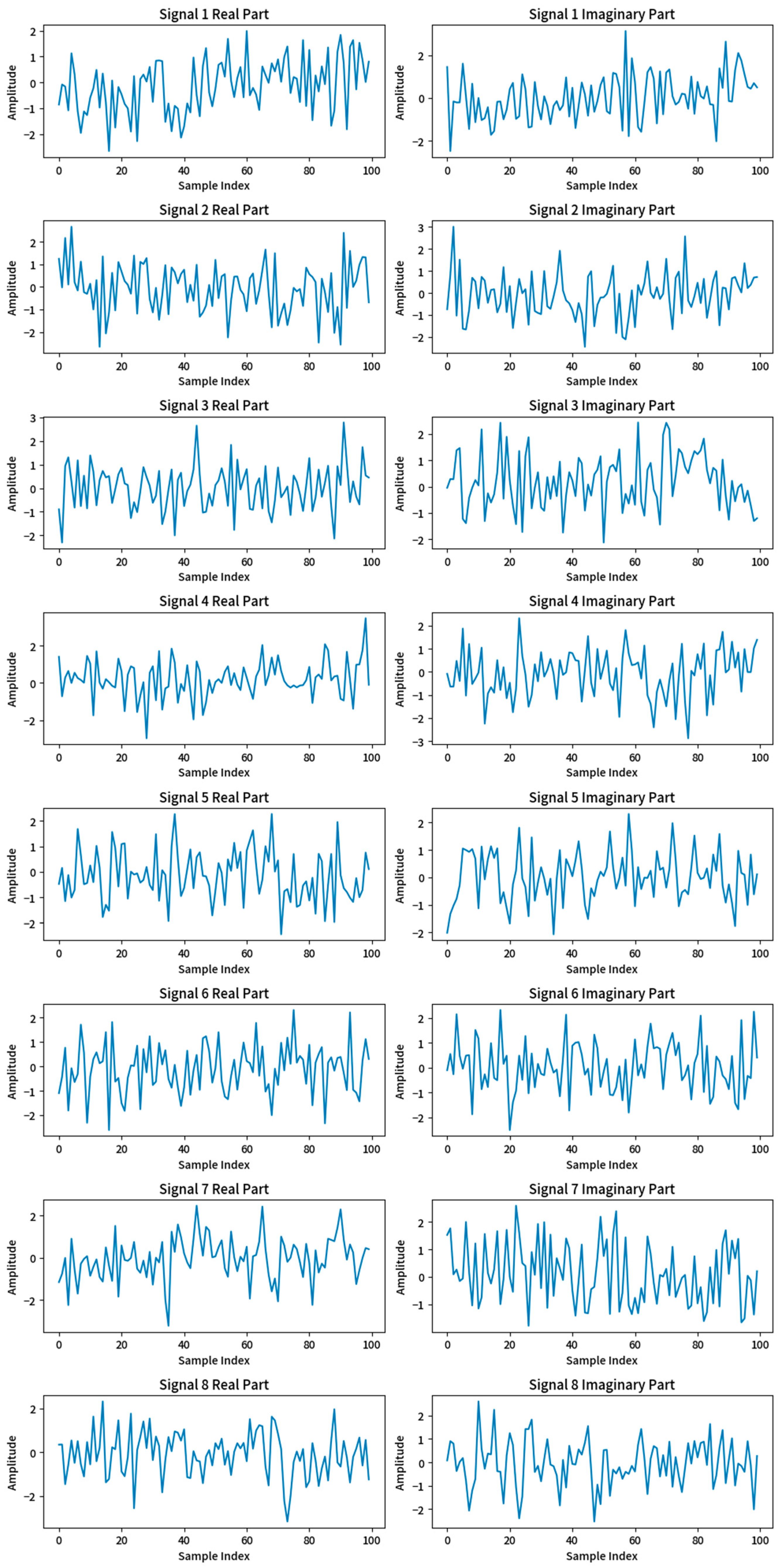
The details of the I/Q data are as follows. The I/Q data are in complex number form and consist of two channels of data, namely the I channel data and the Q channel data. The I channel data are the real part of the complex number, and the Q channel data are the imaginary part of the complex number. An illustration of the I/Q data for each radio presented in Table 5 and Figure 3.

4.2. Data Preprocessing

The real-world dataset is in the .mat file format. The .mat file stores raw I/Q data in a two-dimensional table, with each cell storing the I/Q data for a single sample. The entire table is organized chronologically. Depending on the sampling rate, each transmitter provides 1400–1700 rows of data, with a fixed number of 4096 data columns. Each data cell is stored in a complex format, where the real and imaginary parts represent the I/Q data, respectively. The preprocessing process of the experimental data is depicted in Figure 4.
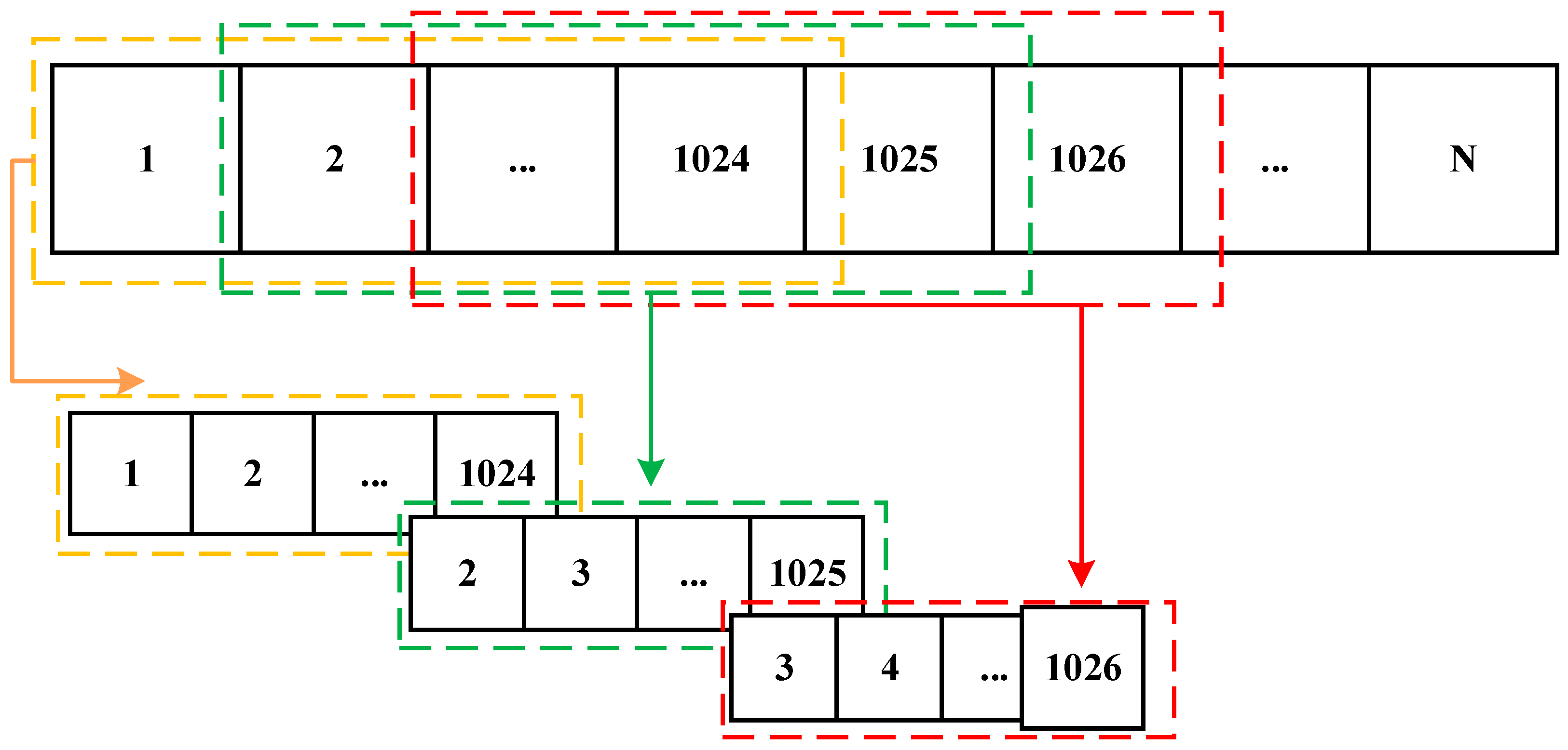
The preprocessing process shown in Figure 3 was implemented in Python. Since the data in the original file are stored as a combination of the real and imaginary parts of I/Q, the preprocessing first involves splitting them into two real-valued I/Q components. Subsequently, the sliding window method was applied to process the raw data and generate more samples. The processing mechanism of the sliding window is illustrated in Figure 5.
Figure 5 demonstrates the operation of a sliding window with a length of 1024 and a sliding step of 1. In this experiment, a window of length 1024 was set to slide and generate samples, including the real-valued I/Q data. Dividing the samples into longer segments can better preserve the device’s inherent fingerprint, reduce the impact of noise, and improve the model’s performance. In the experiment, we set the window movement step size as 128, which could enable the model to detect I/Q damage (e.g., amplitude offset or phase offset) at most locations. After the above window sliding operation, we can use a raw I/Q sequence of length N to produce (N − 1024)/128 + 1 samples.
After sample generation, the data were divided into a training set, a validation set, and a test set at a ratio of 0.7:0.15:0.15. The validation set was used to assess the model’s performance and adjust its hyperparameters, while the test set was solely used for the final evaluation of the model’s performance.

5. Materials and Methods

5.1. Performance Criteria

In order to evaluate the clustering performance of the RF fingerprint blind identification model in an IoMT network, we select a few commonly used evaluation indicators for clustering, including normalized mutual information (NMI), clustering accuracy (ACC), and adjusted Rand index (ARI) [16].
The normalized mutual information (NMI) evaluates the similarity of two clustering results from an information theory perspective, and its formula is
N M I Ω , C = I Ω , C H Ω + H C / 2
where I represents mutual information, H represents the entropy, and the calculation formula for mutual information is
I Ω , C = k j P ω k c j l o g P ω k c j P ω k P c j
where P ω k , P c j , and P ω k c j denote the samples of cluster ω k , the samples of cluster c j , and the samples belonging to both. Mutual information (MI) represents the growth rate of cluster information Ω , which is the rate of uncertainty change of Ω , under the condition that cluster information C has been determined to be generated by clustering. When the mutual information reaches a minimum of 0, it indicates that the current generated cluster is completely random relative to the category, meaning that Ω does not bring any useful information to C when the two are independent. The greater the mutual information, the closer the relationship between Ω and C , and the better the reproduction of Ω to C .
The calculation formula for entropy H is
H Ω = k P ω k l o g P ω k = k ω k N l o g ω k N
The value of NMI is within the range of [0, 1], and the larger its value, the better the clustering effect.
The clustering accuracy (ACC), which is similar to the accuracy in classification problems, is one of the main indicators used to evaluate the clustering effectiveness and is defined as
A C C = i = 1 n δ m a p r i , l i n
where n is the total number of samples, r i is the cluster label predicted by the model for the sample i , l i is the actual category to which sample i belongs, and δ · is an indicator function, which can be expressed as
δ x , y = 1 ,     x = y 0 ,     x y
where m a p · in the formula represents the best class label, which is a mapping from the best predicted cluster to the original cluster, ensuring the optimal clustering accuracy. Generally speaking, the solution of this mapping uses a Hungarian algorithm to obtain the results in polynomial time, and it can dramatically improve the efficiency. Moreover, (15) indicates that the value of ACC is within a range of [0, 1]. A large value of ACC represents a good clustering effect.
The adjusted Rand index (ARI) can be viewed as a modification of the Rand index (RI). The calculation process of the RI is similar to that of the accuracy. In order to illustrate how the ARI and RI are shown in the form of confusion matrices, we firstly define a review of the pair confusion matrix and then calculate the metric.
The calculation formula for the Rand coefficient can be defined as
R I = T P + T N T P + F P + T N + F N
where TP represents the number of two sample points that actually belong to the same type and are also in the same cluster in the prediction results, FP represents the number of two sample points that actually belong to the same class of clusters, TN represents the number of two sample points that actually belong to the same class of clusters, and FN represents the number of cases where two sample points that actually belong to the same type belong to different clusters in the prediction results.
The ARI is an improved version of the RI, aimed at removing the influence of random labels on the RI results. Mathematically, the ARI can be expressed as
A R I = 2 T P · T N F P · F N T P + F N T N + F N + T P + F P T N + F P
The range of ARI values is [−1, 1], and a large value of the ARI indicates a more consistent clustering result.

5.2. Comparison Experiment Using Multiple Benchmark Models

To accurately assess the model’s performance, we select several commonly used clustering models as benchmarks and compare them with the proposed CDAE-DC model. The benchmark models include the k-means model based on principal component analysis (PCA) [2], the convolutional autoencoder (CAE) combined with the k-means model [3], the variational autoencoder (VAE) model [4], the deep embedding clustering (DEC) model [5], and the deep iterative clustering (DC) model [6]. During the experiment, we fine-tune some of these models to ensure their applicability to RF fingerprint data. The performance of each model on our dataset is summarized in Table 6.
In the CDAE-DC model, the parameter selection and changes in the CDAE-DC model tests are as follows. (1) Number of layers: During testing, different numbers of encoder and decoder layers can be applied. We start with a simple two-layer encoder and two-layer decoder and then increase the number of layers up to a four-layer encoder and decoder architecture, since a more complex architecture cannot lead to higher accuracy. (2) Number of neurons per layer: The number of neurons in each layer can vary. For the encoder layers, we compare the values of 128, 256, and 512 neurons, and we finally select 256 neurons, since a more complex architecture cannot lead to higher accuracy. (3) Dropout rate: We compare the dropout rates in the range of 0.1–0.5 and select 0.2 since the random dropout of 20% of the neurons in a layer during training can achieve the highest accuracy. (4) Learning rate: We compare learning rate values including 0.001, 0.0001, etc., and finally select the learning rate of 0.001 since it can achieve the highest accuracy. (5) Batch size: We compare the batch sizes of 32, 64, and 128 and finally select 64 as the batch size since it can achieve the highest accuracy. (6) Number of epochs: We compare the number of epochs using values ranging from 100 to 1000 and finally select 900 epochs, since a larger number cannot improve the accuracy. In summary, we select the “best” result by changing the model architecture to identify the parameters leading to the highest accuracy.
As illustrated in Table 6, the proposed CDAE-DC model demonstrates the optimal identification performance. Benefiting from the guiding function of deep iterative clustering in the representation learning module and the robust representation learning ability of the residual network, CDAE-DC has achieved remarkable improvements in multiple indicators. Thanks to its superior residual network structure and the introduction of reconstruction errors, CDAE-DC can achieve an improvement of 0.203 in the NMI index, 0.193 in the ACC index, and 0.166 in the ARI index. Experiments on real-world datasets have indicated that CDAE-DC can effectively extract the inherent fingerprint features of devices. The extracted fingerprints can reflect the low-dimensional cluster characteristics of devices, thereby achieving better clustering outcomes.
Besides comparing the clustering effects, we also measure the training time of each model during the experimental process, as presented in Table 7. The training duration per round of the contrast clustering model CC-RF is 17 s, which is lower than the 22 s of the iterative clustering model DC and the 19 s of CDAE-DC. However, both the DC and CDAE-DC models are sufficient to converge after 150 rounds of training, while the convergence of CC-RF is relatively difficult and requires 300 epochs of training. Therefore, in terms of the total training time, CC-RF requires 5193 s, which is significantly higher than the 2872 s of DC. From the above analysis, it can be seen that, in an environment with a high signal-to-noise ratio of 10 dB or above, it is suitable to adopt the CDAE-DC model, which is easier to train.
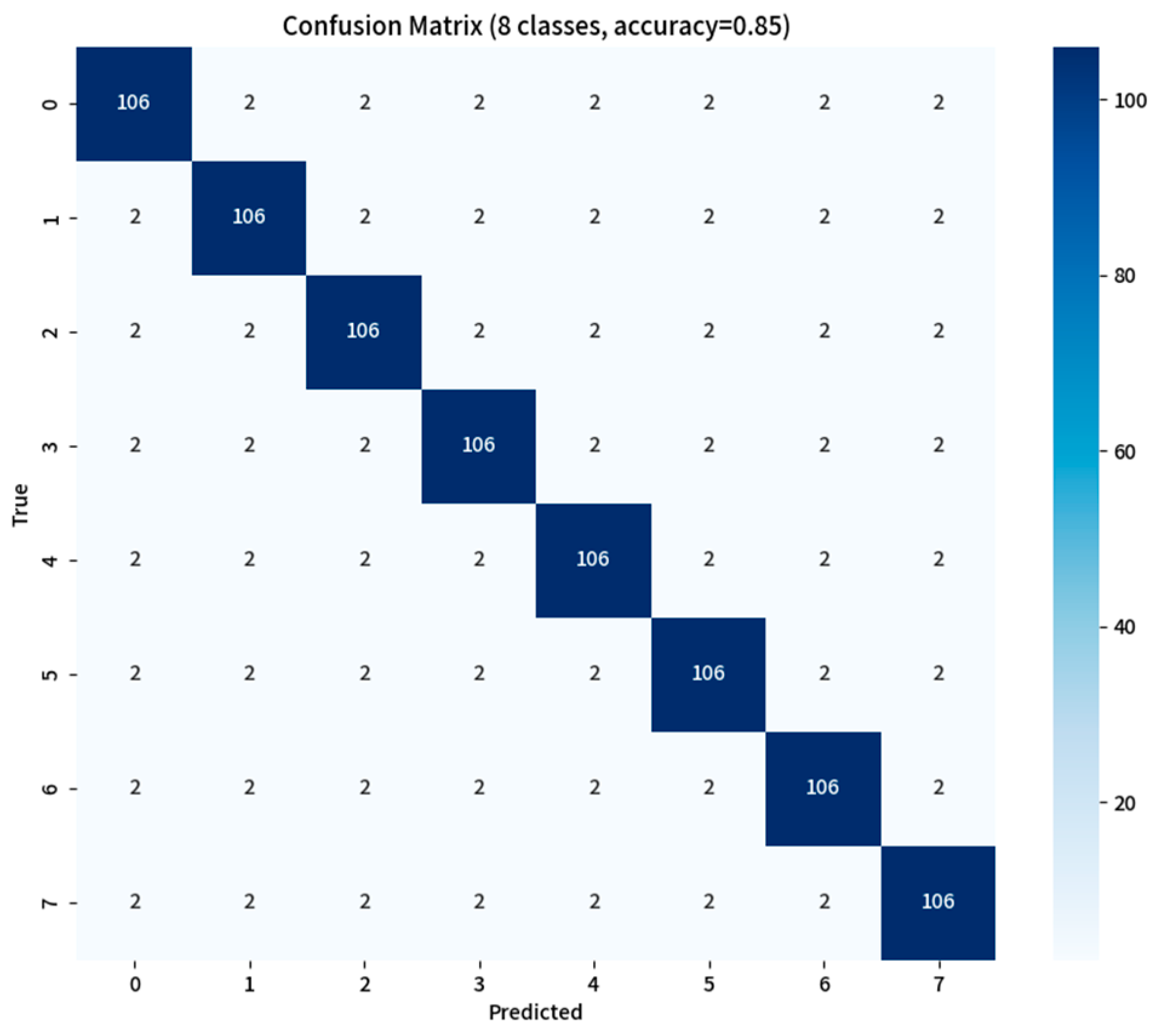
Additionally, we present the ACCs of various models for different SNRs in Table 8. The results show that our proposed CDAE-DC model outperforms the other models at various SNRs. When the SNR = 10 dB, the confusion matrix of CDAE-DC for real-world data is as shown in Figure 6. The accuracy for real-world data is 0.85.
In the CDAE-DC model, the network structure with residual connections plays a crucial role in significantly alleviating the challenges inherent in deep network training. By leveraging this structure, the model effectively shortens the convergence time. This is a remarkable advantage, as it enables the model to reach a stable and optimal state more rapidly during the training process.
To further enhance the clustering effect, in the experiment, the principal component analysis (PCA) technique is employed to reduce the fingerprint dimensions to 256. This dimensionality reduction step is carefully designed to retain the most relevant and discriminative features while reducing the computational complexity.
Notably, the k-means clustering module consumes nearly one-third of the total training time. The reason for this is that each backpropagation operation necessitates the clustering of the entire dataset. This high computational demand of the k-means module highlights the importance of optimizing its performance or exploring alternative clustering algorithms to further improve the overall efficiency of the CDAE-DC model.

6. Conclusions

This paper comprehensively presents the principles, design, and experimental verification of a blind RF fingerprint identification model. This model is based on a noise-reducing self-encoder and deep iterative clustering, aiming to address the security requirements of the Internet of Medical Things (IoMT). Firstly, the overall architecture of the CDAE-DC model is introduced, and the design principles and structures of its various constituent modules are elaborated in detail. The deep clustering model CDAE-DC proposed in this paper has the unique ability to iteratively optimize the representation learning module and the clustering module in an end-to-end manner. This optimization approach enables the propagation of the error loss, which is a significant improvement over traditional methods. As a result, the CDAE-DC model outperforms traditional two-stage clustering methods in terms of performance. Secondly, the CDAE-DC model incorporates the concept of a noise-reducing self-encoder into its encoding–decoding structure. During the training process, the network is optimized by minimizing both the reconstruction error and the classification error simultaneously. This dual-objective optimization strategy helps the model to better extract and utilize the features of RF fingerprints, enhancing its accuracy and robustness. Subsequently, this paper describes the datasets used for model training and testing. These datasets include a real-world dataset generated through the USRP. The use of this dataset allows for a comprehensive evaluation of the model’s performance under different conditions. Finally, the experimental results show that, under different signal-to-noise ratio (SNR) levels, the normalized mutual information (NMI) index of the CDAE-DC model improves by 16–35% compared to the benchmark DC model. In a typical low-SNR IoMT environment, the NMI index of CDAE-DC improves by 0.14–0.25. These results clearly demonstrate that the CDAE-DC model has a good clustering effect and certain anti-noise capabilities, making it a promising solution for RF fingerprint identification in the IoMT security context.
In this study, we only considered the clustering method for the radio-frequency fingerprint recognition of eight devices. When the number of devices increases, the clustering effect will decrease. In future research, we will search for the upper limit of the number of devices that the model proposed in this paper can separate and recognize and explore the performance boundaries of the model.

Author Contributions

Methodology, D.L.; Software, Y.P.; Validation, H.X.; Formal analysis, J.H.; Data curation, S.C. All authors have read and agreed to the published version of the manuscript.

Funding

This study was funded by the National Natural Science Foundation of China (62471090), Central University Fund (ZYGX2024Z016), Sichuan Provincial Natural Science Foundation Project (23NSFSC0422), and Intelligent Terminal Key Laboratory of Sichuan Province (SCITLAB-20005).

Data Availability Statement

Data is unavailable due to privacy.

Conflicts of Interest

The authors declare no conflict of interest.

References

  1. John, S. Radio Frequency Fingerprinting via Deep Learning: Challenges and Opportunities. J. Wirel. Commun. 2023, 15, 123–145. [Google Scholar]
  2. Alwassel, H.; Mahajan, D.; Korbar, B.; Torresani, L.; Ghanem, B.; Tran, D. Self-Supervised Learning by Cross-Modal Audio-Video Clustering. In Proceedings of the Neural Information Processing Systems, NeurIPS, Virtual, 6–12 December 2020; pp. 9758–9770. [Google Scholar]
  3. Xie, J.; Girshick, R.B.; Farhadi, A. Unsupervised deep embedding for clustering analysis. In Proceedings of the International Conference on Machine Learning, New York, NY, USA, 20–22 June 2016; pp. 478–487. [Google Scholar]
  4. Dizaji, K.G.; Herandi, A.; Huang, H. Deep Clustering via Joint Convolutional Autoencoder Embedding and Relative Entropy Minimization. In Proceedings of the 2017 IEEE International Conference on Computer Vision (ICCV), Venice, Italy, 22–29 October 2017; pp. 5736–5745. [Google Scholar]
  5. Guo, X.; Zhu, E.; Liu, X.; Yin, J. Deep Embedded Clustering with Data Augmentation. In Proceedings of the 10th Asian Conference on Machine Learning (ACML), Beijing, China, 14–16 November 2018; pp. 550–565. [Google Scholar]
  6. Huang, P.; Huang, Y.; Wang, W.; Wang, L. Deep Embedding Network for Clustering. In Proceedings of the 2014 22nd International Conference on Pattern Recognition (ICPR), Stockholm, Sweden, 24–28 August 2014; pp. 1532–1537. [Google Scholar]
  7. Zhao, M.; Zhong, S.; Fu, X.; Tang, B.; Pecht, M. Deep Residual Shrinkage Networks for Fault Diagnosis. IEEE Trans. Ind. Inform. 2020, 16, 4681–4690. [Google Scholar] [CrossRef]
  8. Caron, M.; Bojanowski, P.; Joulin, A.; Douze, M. Deep Clustering for Unsupervised Learning of Visual Features. In Proceedings of the European Conference on Computer Vision, Munich, Germany, 8–14 September 2018; Springer: Cham, Switzerland, 2018; pp. 1–6. [Google Scholar]
  9. Rezaei, M.; Dorigatti, E.; Ruegamer, D.; Bischl, B. Learning Statistical Representation with Joint Deep Embedded Clustering. arXiv 2021, arXiv:2109.05232. [Google Scholar]
  10. Li, Y.; Hu, P.; Liu, Z.; Peng, D.; Zhou, J.T.; Peng, X. Contrastive clustering. In Proceedings of the 2021 AAAI Conference on Artificial Intelligence (AAAI), Virtually, 19–21 May 2021. [Google Scholar]
  11. Huang, J.; Gong, S.; Zhu, X. Deep Semantic Clustering by Partition Confidence Maximisation. In Proceedings of the 2020 IEEE/CVF Conference on Computer Vision and Pattern Recognition (CVPR), Seattle, WA, USA, 13–19 June 2020; pp. 8849–8858. [Google Scholar]
  12. Zhong, H.; Chen, C.; Jin, Z.; Hua, X.S. Deep Robust Clustering by Contrastive Learning. arXiv 2020, arXiv:2008.03030. [Google Scholar]
  13. Dilokthanakul, N.; Mediano, P.A.; Garnelo, M.; Lee, M.C.; Salimbeni, H.; Arulkumaran, K.; Shanahan, M. Deep Unsupervised Clustering with Gaussian Mixture Variational Autoencoders. arXiv 2016, arXiv:1611.02648. [Google Scholar]
  14. Jiang, Z.; Zheng, Y.; Tan, H.; Tang, B.; Zhou, H. Variational deep embedding: An unsupervised and generative approach to clustering. In Proceedings of the Twenty-Sixth International Joint Conference on Artificial Intelligence, Melbourne, Australia, 19–25 August 2017; pp. 233–250. [Google Scholar]
  15. Ben-Yosef, M.; Weinshall, D. Gaussian Mixture Generative Adversarial Networks for Diverse Datasets, and the Unsupervised Clustering of Images. arXiv 2018, arXiv:1808.10356. [Google Scholar]
  16. Yu, Y.; Zhou, W.J. Mixture of GANs for Clustering. In Proceedings of the Twenty-Seventh International Joint Conference on Artificial Intelligence IJCAI-18, Stockholm, Sweden, 13–19 July 2018; pp. 3047–3053. [Google Scholar]
  17. Ntelemis, F.; Jin, Y.; Thomas, S.A. Image Clustering Using an Augmented Generative Adversarial Network and Information Maximization. IEEE Trans. Neural Netw. Learn. Syst. 2021, 33, 7461–7474. [Google Scholar] [CrossRef] [PubMed]
  18. Ajagbe, S.A.; Awotunde, J.B.; Adesina, A.O.; Achimugu, P.; Kumar, T.A. Internet of medical things (IoMT): Applications, challenges, and prospects in a data-driven technology. In Intelligent Healthcare: Infrastructure, Algorithms and Management; Springer: Singapore, 2022; pp. 299–319. [Google Scholar]
  19. Chauvin, M.; Piot, O.; Boveda, S.; Fauchier, L.; Defaye, P. Pacemakers and Implantable Cardiac Defibrillators: Must We Fear Hackers? Cybersecurity of Implantable Electronic Devices. Arch. Cardiovasc. Dis. 2023, 116, 51–53. [Google Scholar] [PubMed]
  20. Das, D.; Maity, S.; Chatterjee, B.; Sen, S. Enabling Covert Body Area Network using Electro-Quasistatic Human Body Communication. Sci. Rep. 2019, 9, 4160. [Google Scholar]
  21. Jonathan, Z. Wi-Fi Baby Heart Monitor May Have the Worst IoT Security of 2016-The Register. The Register, 13 October 2016. [Google Scholar]
Figure 1. The structure of the CDAE-DC model.
Electronics 14 01504 g001
Figure 2. CDAE-DC encoder structure.
Electronics 14 01504 g002
Figure 3. Illustration of I/Q data.
Electronics 14 01504 g003
Figure 4. Data preprocessing process.
Electronics 14 01504 g004
Figure 5. Action of sliding the window.
Electronics 14 01504 g005
Figure 6. Confusion matrix of CDAE-DC for real-world data.
Electronics 14 01504 g006
Table 1. Structure of the CDAE-DC encoder.
Layer NameConvolution/PoolingKernelsStep
RSB1(1,6)16(1,1)
RSB2(2,5)32(1,1)
MaxPool1(1,5)-(1,5)
RSB3(1,3)64(1,1)
MaxPool2(1,3)-(1,3)
RSB4(1,3)128(1,1)
MaxPool3(1,3)-(1,3)
Table 2. Structure of the CDAE-DC decoder.
Layer NameConvolution/PoolingKernelsStep
Covn1(1,3)128(1,1)
UpSampling1(1,3)-(1,3)
Covn2(1,3)64(1,1)
UpSampling2(1,5)-(1,5)
Covn3(2,5)32(1,1)
Covn4(1,6)16(1,1)
Table 3. Hardware configuration of the experimental environment.
Hardware NameModel
Server hostingDell T460
Central processing unit (CPU)Intel Xeon Silver 4110
Graphics processing unit (GPU)NVIDIA GeForce GTX1080Ti × 4
Main memory (RAM)DDR4 2666 Mhz, 16G × 4
Hard diskRAID 5 disk array, 20T in total
Covn4(1,6)
Table 4. Software configuration of the experimental environment.
Name of SoftwareVersion
Operating systemUbuntu 20.04.4 LTS
Pycharm2019.3
MATLABR2018a
CUDA11.2
cuDNN8.1.1
Python3.6.5
Keras2.6.0
Tensorflow-gpu2.6.0
Numpy1.19.5
Pandas1.1.5
Scikit-learn0.24.2
Matplotlib3.3.4
Table 5. Details of real-world dataset.
Sample RateDevice NumberNumber of I/Q Samples
1 Gspsdevice16,963,200
device26,963,200
5 Gspsdevice36,553,600
device46,553,600
10 Gspsdevice56,144,000
device66,144,000
15 Gspsdevice75,734,400
device85,734,400
Table 6. Results of model comparison.
Model NameEvaluation Indicator
NMIACCARI
PCA + k-means0.0890.1260.004
CAE + k-means0.2980.3950.265
VAE0.3020.3680.251
DEC0.3850.4360.347
DC0.5260.5980.496
CDAE-DC0.7290.7910.662
Table 7. Training times of each model.
Model NameEpoch TimeTraining Time
PCA + k-means-12 s
CAE + k-means-719 s
VAE18.5 s2961 s
DEC19 s2972 s
DC22 s3364 s
CDAE-DC18 s2872 s
Table 8. Results in terms of ACC for different SNRs.
Model NameSNR [dB]
51015
PCA + k-means0.1170.1260.132
CAE + k-means0.3120.3950.432
VAE0.3010.3680.443
DEC0.3750.4360.454
DC0.52260.5980.612
CDAE-DC0.7010.7910.813
Disclaimer/Publisher’s Note: The statements, opinions and data contained in all publications are solely those of the individual author(s) and contributor(s) and not of MDPI and/or the editor(s). MDPI and/or the editor(s) disclaim responsibility for any injury to people or property resulting from any ideas, methods, instructions or products referred to in the content.